Article

Mathematical Modeling of Toxoplasmosis in Cats with Two Time Delays under Environmental Effects

by
Sharmin Sultana
1,
Gilberto González-Parra
1,* and
Abraham J. Arenas
2
1
Department of Mathematics, New Mexico Tech, Leroy Place, Socorro, NM 87801, USA
2
Departamento de Matemáticas y Estadística, Universidad de Córdoba, Montería 230002, Córdoba, Colombia
*
Author to whom correspondence should be addressed.
Mathematics 2023, 11(16), 3463; https://doi.org/10.3390/math11163463
Submission received: 24 July 2023 / Revised: 6 August 2023 / Accepted: 8 August 2023 / Published: 10 August 2023
(This article belongs to the Special Issue Applied Mathematical Modelling and Dynamical Systems)

Abstract

:
In this paper, we construct a more realistic mathematical model to study toxoplasmosis dynamics. The model considers two discrete time delays. The first delay is related to the latent phase, which is the time lag between when a susceptible cat has effective contact with an oocyst and when it begins to produce oocysts. The second discrete time delay is the time that elapses from when the oocysts become present in the environment to when they are able to infect. The main aim in this paper is to find the conditions under which the toxoplasmosis can disappear from the cat population and to study whether the time delays can affect the qualitative properties of the model. Thus, we investigate the impact of the combination of two discrete time delays on the toxoplasmosis dynamics. Using dynamical systems theory, we are able to find the basic reproduction number R 0 d that determines the global long-term dynamics of the toxoplasmosis. We prove that, if R 0 d < 1 , the toxoplasmosis will be eradicated and that the toxoplasmosis-free equilibrium is globally stable. We design a Lyapunov function in order to prove the global stability of the toxoplasmosis-free equilibrium. We also prove that, if the threshold parameter R 0 d is greater than one, then there is only one toxoplasmosis-endemic equilibrium point, but the stability of this point is not theoretically proven. However, we obtained partial theoretical results and performed numerical simulations that suggest that, if R 0 d > 1 , then the toxoplasmosis-endemic equilibrium point is globally stable. In addition, other numerical simulations were performed in order to help to support the theoretical stability results.

1. Introduction

T. gondii is a protozoan parasite that attacks and parasitizes animals including humans. Its only definitive hosts are members of the family Felidae. However, other species are intermediate hosts [1,2,3]. In humans, immunocompromised and congenitally infected persons can suffer from severe and lethal effects [4,5]. In individuals who are immunocompetent, toxoplasmosis infection usually only causes flu symptoms and chorioretinitis [4,6,7]. However, severe acute toxoplasmosis has been reported in immunocompetent persons [8]. In addition, it has been suggested that T. gondii infection might cause autoimmune diseases and neurological disorders [9,10,11,12,13]. It has been found that the genotype of the strain of T. gondii affects the severity of the infection [14,15,16].
T. gondii is one of the most significant foodborne pathogens [4,17,18,19]. In the USA alone, there are more than 40 million people with T. gondii [4,17]. It has been estimated that more than 60% of some communities around the world are affected. Prevalence is higher in regions that are hot, humid, and at lower altitudes [4,20]. For instance, in tropical South America, T. gondii has higher genetic diversity [16]. It has been estimated that 32% of the total consequences of toxoplasmosis are due to congenital toxoplasma infections [21]. Toxoplasmosis exists in all the countries around the world and it has been estimated that there are 190,000 congenital toxoplasmosis cases annually (1.5 per 1000 live births) [22,23]. However, the estimation related to acquired toxoplasmosis is uncertain. In the United States, it has been estimated that there are 58 congenital toxoplasmosis cases per 100,000 individuals [22,24]. It has also been estimated that, in the United States, the annual cost associated with T. gondii is 10,964 quality-adjusted life-years (ranking it third among food-related pathogens) and the cost of illness is USD 2.9 billion (ranked second) [22,25]. High associated costs are present in South America and in some low-income countries [22,23].
There are different routes of transmission of T. gondii; ingestion of sporulated oocysts, ingestion of viable tissue cysts, and congenital infection. For instance, the number of congenital toxoplasmosis infections has been estimated to be 1.2 million [26]. Oocyst contamination in fruits and greens contributes significantly more to total estimated T. gondii infections than bradyzoite-contaminated foods [19]. The infected cats are able to shed oocysts in the environment and humans can be infected after consumption of undercooked and raw meat [19,20,27,28,29,30]. It has been estimated that the feces of cats shedding T. gondii have 2.5 × 10 6 oocysts/gr and a cat sheds around 20 million oocysts per day [31]. The control of toxoplasmosis and the definitive host is a challenging problem [30,32,33,34,35]. Current health interventions are weak since they only focus on acute/reactivated forms of the disease [5,30]. Thus, studies related to toxoplasmosis interventions are crucial and worthwhile.
Animals usually do not suffer from symptoms related to toxoplasmosis infection [36,37,38,39]. However, they suffer from congenital transmission and its consequences, such as offspring with abnormalities [30]. Documentation of the consequences of T. gondii infection in animals has been presented [4,36,37,38,40,41]. Toxoplasmosis infections in many different animals have important consequences from different viewpoints [36,41,42,43,44]. Also, economic and public health impacts related to toxoplasmosis have been mentioned in the literature [30,45,46].
There have been several previous studies devoted to investigating toxoplasmosis dynamics [26,47]. Some of these works have used mathematical models with a variety of approaches [26]. Few mathematical models have focused on investigating cat–human transmission under different assumptions related to demographic factors [48,49]. However, there are other, more complex models that have been employed to study the dynamics of toxoplasmosis using other variables and hosts [47,50,51,52,53]. In addition, some researchers have investigated and explored the effect of cat and swine vaccinations [32,33,47,50,51,54]. Also, within-host mathematical models have been proposed to study the T. gondii dynamics within the host [55]. In [26], an excellent overview of mathematical models for toxoplasmosis dynamics is provided.
In this paper, we study the effects of the combination of two time delays on the dynamics of toxoplasmosis, taking into account the cat population and the number of oocysts in the environment. The introduction of two time delays allow us to study a more realistic scenario despite the typical limitations of mathematical models for real-world processes. One time delay is related to the cats’ exposed stage and the second delay is related to the time it takes an oocyst to become infectious after being shed by the cat. In particular, the first discrete time delay occurs due to the fact that, when a susceptible cat has effective contact with an oocyst, that cat starts an incubation period before being able to start shedding oocysts. Thus, the time delay is the incubation period of the cat. In order to study the aforementioned effects, we construct a mathematical model that uses a nonlinear system of delay differential equations. One key aspect of the model is the fact that, once the cats have effective contact with the oocysts, they are not able to produce oocysts instantaneously [2,6,20]. The inclusion of oocysts is crucial since they are highly responsible for the persistence of the T. gondii [2,6,20,27,29,56,57]. The constructed model encompasses the fact that cats can get the T. gondii parasite through effective contact with an oocyst. The model is more realistic than the mathematical model presented in [47]. This previous model does not include any time delay related to more realistic scenarios. There is a delay in the shedding of oocysts that lasts between 3 and 30 days after ingestion of tissue cysts [6,58,59]. The constructed model also includes the cats due to their importance in the reproduction of T. gondii and therefore for the toxoplasmosis disease [60]. Public health policies should take into account many factors to control the spread of toxoplasmosis; for instance, domestic cats and other intermediate hosts [43]. There are three major genotypes (type one, type two, and type three) of T gondii. In Europe and the USA, type two is the most prevalent for congenital toxoplasmosis. Their pathogenicity differs, but if we assume an average for all the types, then the model proposed in this study will be applicable. However, if we differentiate the genotypes and their features regarding pathogenicity then a more complex model will be required [61,62,63].
Mathematical models based on systems of delay differential equations have been used to study different kind of infectious diseases, including between hosts and within hosts [64,65,66,67,68,69,70,71,72,73]. The reason for including time delays is the fact that many processes do not have instantaneous effects in the real world. However, there are some drawbacks of employing mathematical models with delay differential equations. For instance, their analysis is usually more challenging and cumbersome. Furthermore, solving delay differential equations is more difficult than ordinary differential equations [74,75,76,77]. The inclusion of delays in the differential equations can have a great impact on the stability of the steady states and oscillatory behavior can appear with some particular values of the time delays [78,79,80,81,82,83,84,85]. Moreover, the inclusion of multiple time delays makes the mathematical analysis more complex and oftentimes intractable [86,87,88,89,90,91]. In particular, there are several works that have studied mathematical models that have two time delays [92,93,94]. For instance in [95], the authors used two time delays in a model to study the control of disease spreading in networks.
In summary, in our study, one main objective is to investigate the effect of the combination of two time delays on the toxoplasmosis infection dynamics. The importance of the combination of two time delays resides in the fact that, if a stability switch occurs in the model with only one time delay, then it might be possible that the result does not hold for the model with two time delays (see [81,96]). Moreover, the model with two time delays is closer to reality and also provides helpful insight into the mechanism of more complex dynamics [92]. Therefore, we investigate if the time delays are able to produce different behaviors and complexity in the toxoplasmosis dynamics. We explore the stability of the steady states of the model. We prove that, if R 0 d is greater than one, then there is only one toxoplasmosis-endemic equilibrium point, but due to the presence of two discrete time delays, we are not able to prove its stability. However, we obtained partial theoretical results and performed numerical simulations that suggest that, if R 0 d > 1 , then the point is globally stable. We also performed in silico simulations to support the theoretical results. In addition, we simulated some scenarios to gain insight into the effect of the two time delays on the toxoplasmosis dynamics.

2. Mathematical Model

We designed a new mathematical model to explore and investigate the dynamics of toxoplasmosis in a population of cats. The proposed model includes two discrete time delays, which makes the model closer to reality. The first delay is related to the time that it takes for a cat to become infected after infectious contact with the oocysts. In particular, the first discrete time delay is the incubation period before the cats start shedding oocysts. Thus, the term β S ( t ) O ( t ) represents that the cats have effective contact with the oocysts at time t and the term β S ( t τ 1 ) O ( t τ 1 ) e μ τ 1 represents the cats leaving the incubation phase (after a time τ 1 ) and becoming able to shed oocysts [69,97]. The second time delay is related to the time that it takes the oocysts to sporulate and become infectious (somewhere between 1 and 5 days) after they are shed in the environment by an infected cat [6,20,56,58]. The mathematical model includes vaccinated cats and infected cats [32,47,98]. The cats get infected by contact with oocysts. These infections depend on the amount of T. gondii in the environment [54]. The model uses a system of delay differential equations. Further details regarding the model can be seen in [47].
The model has five subpopulations: susceptible S ( t ) , latent E ( t ) , infected I ( t ) , vaccinated–recovered V R ( t ) , and oocysts O ( t ) . The vaccine provides life immunity [32,33,99,100]. A susceptible cat goes to the latent stage after contact with an oocyst. The infected cats stay in this stage for a mean time of 1 α . The change in the number of oocysts in the environment is proportional to the infectious cats I ( t ) . The oocysts in the environment suffer from natural degradation.
The mathematical model is given in terms of the following nonlinear delay differential equation system
S ˙ ( t ) = μ ( 1 I ( t ) ) β S ( t ) O ( t ) ( μ + γ ) S ( t ) , E ˙ ( t ) = β S ( t ) O ( t ) β S ( t τ 1 ) O ( t τ 1 ) e μ τ 1 μ E ( t ) , I ˙ ( t ) = β S ( t τ 1 ) O ( t τ 1 ) e μ τ 1 α I ( t ) , V R ˙ ( t ) = α I ( t ) + γ S ( t ) μ V R ( t ) , O ˙ ( t ) = k I ( t τ 2 ) μ 0 O ( t ) .
We assume that the total population of cats is given by N ( t ) = S ( t ) + E ( t ) + I ( t ) + V R ( t ) = 1 (without loss of generality). Therefore, since the state variable V R is not included explicitly in the first three parts of model (1), we can analyze the model without this variable. The graphical representation of mathematical model (1) can be observed in Figure 1. Note that vertical transmission is included in the cat population [28,40,101,102,103,104].
For the sake of simplicity, model (1) can be studied using the following simplified system
S ˙ ( t ) = μ ( 1 I ( t ) ) β S ( t ) O ( t ) ( μ + γ ) S ( t ) , E ˙ ( t ) = β S ( t ) O ( t ) β S ( t τ 1 ) O ( t τ 1 ) e μ τ 1 μ E ( t ) , I ˙ ( t ) = β S ( t τ 1 ) O ( t τ 1 ) e μ τ 1 α I ( t ) , O ˙ ( t ) = k I ( t τ 2 ) μ 0 O ( t ) ,
where the parameters μ , γ , τ 1 , τ 2 , β , α , k are all positive. Consider
R + 4 = ( x 1 , x 2 , x 3 , x 4 ) : x i 0 , i = 1 , , 4 .
In order to investigate the existence and uniqueness of model (2), we denote by C [ τ , 0 ] , R + 4 (with τ = max τ 1 , τ 2 ) the Banach space of continuous functions ζ defined in ζ : [ τ , 0 ] R + 4 such that ζ ( t ) = ζ 1 ( t ) , ζ 2 ( t ) , ζ 3 ( t ) , ζ 4 ( t ) and a norm defined by (see [105])
ζ = sup τ s 0 ζ 1 ( s ) , ζ 2 ( s ) , ζ 3 ( s ) ζ 4 ( s ) .
Thus, for biological significance, we further assume that the initial conditions of model (2) have the following structure:
S ( s ) = ζ 1 ( s ) > 0 , E ( s ) = ζ 2 ( s ) 0 , I ( s ) = ζ 3 ( s ) 0 , O ( s ) = ζ 4 ( s ) 0 , s [ τ , 0 ] , S ( 0 ) = S 0 = ζ 1 ( 0 ) , E ( 0 ) = E 0 = ζ 2 ( 0 ) , I ( 0 ) = I 0 = ζ 3 ( 0 ) , O ( 0 ) = O 0 = ζ 4 ( 0 ) .
Moreover, for the continuity of the initial conditions, it is required that
E ( 0 ) = τ 0 ζ 1 ( w ) ζ 4 ( w ) e μ w d w .
The initial value of E ( 0 ) must be related to the initial values of the variables S and O such that they satisfy the conditions in Equation (3), which is an integral constraint of the function ζ 2 : [ τ , 0 ] [ 0 , ] , and this is important so that the positivity of the solutions is preserved [106]. From the theory of functional differential equations [107], we can apply the theorem that comes next.
Theorem 1.
Suppose O is an open set in R × C [ τ , 0 ] , R + 4 , f : Ω R 4 is continuous, and f ( t , ζ ) is Lipschitzian in ζ in each compact set in Ω . If ( σ , φ ) Ω , then there is a unique solution to model (2) through ( σ , φ ) .
Proof. 
See [107] (p. 44). □
Therefore, it follows that model (2) admits a unique solution provided that the conditions shown in Equation (3) hold.
Next, the positivity and boundedness for model (2) are established with the subsequent theorem.
Theorem 2.
The solution X ( t ) = ( S ( t ) , E ( t ) , I ( t ) , O ( t ) ) to Equation (2) is positive and uniformly bounded on [ 0 , + ) if Equation (3) holds.
Proof. 
From Equation (2), one can find that
S ˙ ( t ) = μ ( 1 I ( t ) ) β S ( t ) O ( t ) γ S ( t ) β S ( t ) O ( t ) γ S ( t ) .
Thus,
S ( t ) S ( 0 ) exp 0 t ( β O ( s ) + γ ) d s > 0 , t 0 .
To show that the other variables preserve positivity over time, we proceed using the method of steps [106]. With this order of ideas, let t [ 0 , τ ] . With the initial conditions shown in Equation (3), it follows that S ( t τ ) O ( t τ ) 0 in this interval. Then, from the third equation of system (2), and using the comparison criterion for differential equations, it follows that I ( t ) 0 for all t ( 0 , τ ] . Analogously, it is verified that O ( t ) > 0 with t ( 0 , τ ] , and, therefore, the non-negativity for E ( t ) is a consequence of the simple fact that the solution of the differential equation related to E ( t ) can be written as
E ( t ) = e μ t E ( 0 ) + t τ t S ( w ) O ( w ) e μ w d w , t ( 0 , τ ] .
The above reasoning can be applied for variables E , I , O in the interval ( τ , 2 τ ] and successively in intervals of the form ( n τ , ( n + 1 ) τ ] , for n N 0 . Next, from system (2), one gets
S ˙ ( t ) + E ˙ ( t ) + I ˙ ( t ) + O ˙ ( t ) μ + k M ( S ( t ) + E ( t ) + I ( t ) + O ( t ) ) ,
where M < min μ + γ , μ , α + μ , μ 0 . As a result, one obtains
lim sup t ( S ( t ) + E ( t ) + I ( t ) + O ( t ) ) μ + k M .
Hence, we study the qualitative behavior of model (2) in the following region:
R = ( S , E , I , O ) R + 4 : 0 < S ( t ) + E ( t ) + I ( t ) + O ( t ) μ + k M ,
where R + 4 denotes the non-negative cone of R 4 . Thus, the set R is positively invariant. □
Now, we can focus on the stability analysis of model (2) in the restricted region R .

3. Stability Analysis of the Model

The qualitative analysis of the mathematical model from Equation (2) can be undertaken by using linearizations and finding suitable Lyapunov functions [105,108]. Before we begin the stability analysis, we would like to prove the positivity and boundedness of the solutions to model (2).

3.1. Disease-Free Steady State for the Model without Delay

The steady states of model (2) without delay are the same as for the model with the two time delays τ 1 and τ 2 . The steady states are crucial for the study of dynamical systems [108,109,110].
We can start analyzing the stability of the steady states of the model without considering the delays. This analysis has been performed previously and the details can be seen in [47,111,112]. The model from Equation (2) without delay has a toxoplasmosis-free equilibrium point F * and a toxoplasmosis-endemic equilibrium point. The toxoplasmosis-free equilibrium point is given by
F * = μ μ + γ , 0 , 0 , 0 .
It has also been found that the basic reproduction number for model (2) without any time delays is given by [47,52,111]:
R 0 = k β μ α μ 0 γ + μ .
If R 0 < 1 , the toxoplasmosis-free equilibrium point is globally asymptotically stable. On the other hand, the toxoplasmosis-free equilibrium point F * is unstable when R 0 > 1 [47,52,53].

3.2. Endemic Steady State

Model (2) also has a unique toxoplasmosis-endemic equilibrium point. It is important to determine this endemic point for the stability analysis of model (2). Indeed, the toxoplasmosis-endemic equilibrium point is given by E P * = S * , E * , I * , O * , where
S * = α μ 0 β k e μ τ 1 , E * = α μ k β e μ τ 1 + α γ μ 0 + α μ 0 μ e μ τ 1 1 β k e μ τ 1 μ e μ τ 1 + α μ = α 2 μ 0 ( γ + μ ) 1 e μ τ 1 R 0 d 2 1 β k e μ τ 1 μ e μ τ 1 + α μ , I * = μ k β e μ τ 1 + α γ μ 0 + α μ 0 μ β μ e μ τ 1 + α k = α μ 0 ( γ + μ ) R 0 d 2 1 β μ e μ τ 1 + α k , O * = μ k β e μ τ 1 + α γ μ 0 + α μ 0 μ β μ 0 μ e μ τ 1 + α = α ( γ + μ ) R 0 d 2 1 β μ e μ τ 1 + α ,
and where we define
R 0 d = μ k β e μ τ 1 μ 0 γ + μ α .
Thus, this toxoplasmosis-endemic equilibrium makes biological sense if R 0 d > 1 . Moreover, note that E P * is biologically feasible iff R 0 d 1 . In particular, if R 0 d = 1 , the point E P * collides with F * . Now, we proceed to study model (2), which contains two discrete time delays τ 1 and τ 2 .

3.3. Toxoplasmosis-Free Steady State Analysis

The steady states of model (2) can be found by setting the right-hand side as equal to zero and setting any state variable with delay as a state variable without delay. To study the stability of the toxoplasmosis-free steady state, we linearize system (2). The following is the characteristic equation:
| J 0 + J τ 1 e λ τ 1 + J τ 2 e λ τ 2 λ I | = 0 ,
where
J 0 = γ μ 0 μ β μ γ + μ 0 μ 0 β μ γ + μ 0 0 α 0 0 0 0 μ 0 , J τ 1 = 0 0 0 0 0 0 0 β μ e μ τ 1 γ + μ 0 0 0 β μ e μ τ 1 γ + μ 0 0 0 0 , J τ 2 = 0 0 0 0 0 0 0 0 0 0 0 0 0 0 k 0
As a result, the transcendental characteristic equation is given by
| J 0 + J τ 1 e λ τ 1 + J τ 2 e λ τ 2 λ I | = λ + μ λ + γ + μ T λ = 0 ,
where,
T λ = γ + μ λ 2 + γ α + α μ + γ μ 0 + μ μ 0 λ e λ τ 1 β μ e μ τ 1 e λ τ 2 k + α γ μ 0 + α μ 0 μ = γ + μ λ 2 + γ + μ μ 0 + α λ e λ τ 1 β μ e μ τ 1 e λ τ 2 k + α μ 0 γ + μ = γ + μ λ 2 + μ 0 + α λ α μ 0 R 0 d 2 e λ ( τ 1 + τ 2 ) + α μ 0 .
It is clear from Equation (8) that two eigenvalues are λ 1 = μ and λ 2 = μ γ . The other eigenvalues are given by the roots of T λ . We propose the following theorem.
Theorem 3.
The toxoplasmosis-free equilibrium F * of model (2) is locally asymptotically stable if R 0 d < 1 but unstable if R 0 d > 1 .
Proof. 
Suppose that one eigenvalue λ has a non-negative real part. Then, T ( λ ) = 0 can be written as
λ 2 + λ ( α + μ 0 ) + α μ 0 = α μ 0 R 0 d 2 e λ τ 1 + τ 2 .
The modulus of the left-hand side of Equation (9) satisfies
| λ 2 + λ ( α + μ 0 ) + α μ 0 |   α μ 0 .
On the other hand, the modulus of the right-hand side of Equation (9) satisfies
| α μ 0 R 0 d 2 e λ τ 1 + τ 2 |   < α μ 0 R 0 d 2 < α μ 0 ,
if R 0 d < 1 . Then, Equation (9) with inequalities (10) and (11) lead to a contradiction. It follows that all the roots of the characteristic Equation (8) have a negative real part. Thus, the toxoplasmosis-free equilibrium point is locally asymptotically stable whenever R 0 d < 1 . □
Now that we have obtained the local stability of the equilibrium point F * , we can proceed to investigate its global stability.

3.4. Global Stability Analysis of the Toxoplasmosis-Free Equilibrium F *

We can try to investigate the global stability of F * by using the Lyapunov theorem or the LaSalle variance principle [113]. Let us propose the following theorem.
Theorem 4.
The toxoplasmosis-free equilibrium point F * of system (2) is globally asymptotically stable in R if R 0 d < 1 .
Proof. 
Denoting y t as the translation of the solution to system (2), we have that y t = ( S ( t + ξ ) , I ( t + ξ ) , V ( t + ξ ) ) where ξ [ τ , 0 ] . Let us propose the following Lyapunov function:
L ( I ( t ) , S ( t ) , O ( t ) ) = β t τ 1 t S ( ξ ) O ( ξ ) e μ τ 1 d ξ + α t τ 2 t I ( ξ ) d ξ + I ( t ) + α k O ( t ) .
Note that, at F * , one has that S * = μ μ + γ ,   I * = 0 ,   O * = 0 and therefore L ( F * ) = 0 . The Lyapunov function L satisfies
L ( I ( t ) , S ( t ) , O ( t ) ) > 0 ,
at any point different from F * . The time derivative of L ( I ( t ) , S ( t ) , O ( t ) ) through the trajectories of model (2) is given by
L = β e μ τ 1 S ( t ) O ( t ) S ( t τ ) O ( t τ ) + α ( I ( t ) I ( t τ 2 ) ) + I ( t ) + α k O ( t ) = β e μ τ 1 S ( t ) O ( t ) S ( t τ 1 ) O ( t τ 1 ) + α ( I ( t ) I ( t τ 2 ) ) + α I ( t τ 2 ) α μ 0 k O ( t ) = β e μ τ 1 S ( t ) O ( t ) α μ 0 k O ( t ) β μ μ + γ O ( t ) e μ τ 1 α μ 0 k O ( t ) = α μ 0 k O ( t ) μ β k e μ τ 1 α μ 0 ( μ + γ ) 1 = α μ 0 k O ( t ) ( R 0 d 2 1 ) ,
since, from first equation of system (2), one can deduce that S ( t ) μ μ + γ . Thus, one gets
L α μ 0 k O ( t ) ( R 0 d 2 1 ) .
Therefore, L 0 if R 0 d 1 . Using LaSalle’s invariance principle, one finds that F * is globally asymptotically stable (GAS) in R . □

3.5. Stability Analysis of the Toxoplasmosis-Endemic Steady State

The characteristic equation for the toxoplasmosis-endemic steady state is given by
| J E + J τ 1 e λ τ 1 + J τ 2 e λ τ 2 λ I | = 0 ,
where
J E = β O * γ μ 0 μ β S * β O * μ 0 β S * 0 0 α 0 0 0 0 μ 0 , J τ 1 = 0 0 0 0 β O * e μ τ 1 0 0 β S * e μ τ 1 β O * e μ τ 1 0 0 β S * e μ τ 1 0 0 0 0 ,   and   J τ 2 = 0 0 0 0 0 0 0 0 0 0 0 0 0 0 k 0 .
The explicit form of Equation (14) is
μ + λ ( S * e λ τ 1 λ τ 2 μ τ 1 γ β k + β k λ + β k μ + O * e τ 1 μ + λ β λ μ + O * e τ 1 μ + λ β μ μ 0 + O * α β λ + O * α β μ 0 + O * β λ 2 + O * β λ μ 0 + γ α λ + α γ μ 0 + λ 2 α + α λ μ + α λ μ 0 + α μ 0 μ + γ λ 2 + γ λ μ 0 + λ 3 + λ 2 μ + λ 2 μ 0 + λ μ μ 0 ) = 0 .
Clearly, one eigenvalue is λ = μ . The other eigenvalues are the roots of the following equation
k S * β μ + γ + λ e τ 1 τ 2 λ μ τ 1 μ 0 + λ e τ 1 μ + λ β μ O * + α + λ β O * + γ + λ + μ = 0 .
Let us assume that a root λ of this equation has a non-negative real part. Thus, Equation (15) can be rewritten as
μ 0 + λ e τ 1 μ + λ β μ O * = k S * β μ + γ + λ e τ 1 τ 2 λ μ τ 1 + μ 0 + λ α + λ β O * + γ + λ + μ .
The modulus of the left-hand side of this last equation satisfies
μ 0 + λ e τ 1 μ + λ β μ O * = μ 0 + λ e μ τ 1 β μ O * e τ 1 λ = μ 0 + λ e μ τ 1 β μ e τ 1 λ α ( γ + μ ) R 0 d 2 1 β μ e μ τ 1 + α < μ 0 + λ α ( γ + μ ) R 0 d 2 1 .
Now, the modulus of the right-hand side of Equation (15) satisfies
k S * β μ + γ + λ e τ 1 τ 2 λ μ τ 1 + μ 0 + λ α + λ β O * + γ + λ + μ > μ 0 + λ α + λ β O * + γ + λ + μ k S * β μ + γ + λ e τ 1 τ 2 λ μ τ 1 > γ + λ + μ μ 0 α k S * β e μ τ 1 e τ 1 τ 2 λ > γ + μ μ 0 α k α μ 0 β k e μ τ 1 β e μ τ 1 e τ 1 τ 2 λ = γ + μ μ 0 α 1 e τ 1 τ 2 λ .
Accordingly, one gets that
μ 0 + λ α ( γ + μ ) R 0 d 2 1 > γ + μ μ 0 α 1 e τ 1 τ 2 λ
i.e.,
μ 0 + λ R 0 d 2 1 > μ 0 1 e τ 1 τ 2 λ , R 0 d > 1 .
Thus, as R 0 d 1 + , we have a contradiction. Therefore, λ cannot have a positive real part.
Now, Equation (15) can be rewritten as
( μ 0 + λ ) ( α + λ ) ( β O * + γ + μ + λ ) + β μ O * ( μ 0 + λ ) e μ τ 1 λ τ 1 β k S * ( γ + μ + λ ) e μ τ 1 λ τ 1 λ τ 2 = 0 .
Equation (16) is a function of λ , τ 1 , and τ 2 with the following form
P ( λ , τ 1 , τ 2 ) = P 0 ( λ ) + P 1 ( λ ) e λ τ 1 + P 2 ( λ ) + P 3 ( λ ) e λ τ 1 e λ τ 2 ,
where P 0 ( λ ) = ( μ 0 + λ ) ( α + λ ) ( β O * + μ + γ + λ ) . It is clear that the degree of P 0 ( λ ) is three. The other polynomials P i ( λ ) are given by P 1 ( λ ) = β μ ( μ 0 + λ ) O * e μ τ 1 , P 2 ( λ ) = 0 , and P 3 ( λ ) = α μ 0 γ + λ + μ . Notice that
d e g ( P 0 ( λ ) ) m a x { d e g ( P 1 ( λ ) ) , d e g ( P 2 ( λ ) ) , d e g ( P 3 ( λ ) ) } ,
and
i = 0 3 P i ( 0 ) = μ 0 α ( β O * + μ + γ ) + β μ μ 0 O * e μ τ 1 α μ 0 γ + μ .
The parameters of model (2) satisfy α > 0 , μ 0 > 0 , μ > 0 , and β > 0 ; then, the above expression will be zero if O * = 0 . Note that if O * is a component of the endemic equilibrium point E P * , then O * cannot be equal to zero. Hence, the above expression cannot be zero. Thus, one gets that
P 0 ( 0 ) + P 1 ( 0 ) + P 2 ( 0 ) + P 3 ( 0 ) 0 .
Therefore, λ = 0 cannot be an eigenvalue or a root of Equation (14). Note that the polynomials P 0 , P 1 , P 2 , and P 3 do not have common zeros. On the other hand, the polynomials P 0 ( λ ) , P 1 ( λ ) , P 2 ( λ ) , and P 3 ( λ ) hold with
lim λ P 1 ( λ ) P 0 ( λ ) + P 2 ( λ ) P 0 ( λ ) + P 3 ( λ ) P 0 ( λ ) < 1 .
Therefore, Equation (17) is a characteristic equation (see [93]).
To study stability switching, we consider purely imaginary characteristic roots since λ 0 and roots of a real function always occur as conjugate pairs. Let us assume that λ = i ω ( ω > 0 ) is an eigenvalue. Substituting this into Equation (17), one obtains
P ( i ω , τ 1 , τ 2 ) = P 0 ( i ω ) + P 1 ( i ω ) e i ω τ 1 + P 2 ( i ω ) + P 3 ( i ω ) e i ω τ 1 e i ω τ 2 = 0 .
Since P 2 ( i ω ) = 0 and e i ω τ 2 = 1 , it follows that
| | P 0 ( i ω ) + P 1 ( i ω ) e i ω τ 1 | | = | | P 3 ( i ω ) e i ω τ 1 | | = | | P 3 ( i ω ) | | .
Then, the above equation can be written as
( P 0 ( i ω ) + P 1 ( i ω ) e i ω τ 1 ) ( P 0 ¯ ( i ω ) + P 1 ¯ ( i ω ) e i ω τ 1 ) = ( P 3 ( i ω ) e i ω τ 1 ) ( P 3 ¯ ( i ω ) e i ω τ 1 ) .
After simplifying, one gets
P 0 ( i ω ) 2 + P 1 ( i ω ) 2 P 3 ( i ω ) 2 = 2 R e ( P 0 ( i ω ) P 1 ¯ ( i ω ) ) cos ( ω τ 1 ) + 2 I m ( P 0 ( i ω ) P 1 ¯ ( i ω ) ) sin ( ω τ 1 ) .
Hence,
P 0 ( i ω ) 2 + P 1 ( i ω ) 2 P 3 ( i ω ) 2 = 2 A 1 ( i ω ) cos ( ω τ 1 ) 2 B 1 ( i ω ) sin ( ω τ 1 ) ,
where
A 1 ( i ω ) = R e ( P 0 ( i ω ) P 1 ¯ ( i ω ) ) and B 1 ( ω ) = I m ( P 0 ( i ω ) P 1 ¯ ( i ω ) ) .
Suppose that there exists ω such that A 1 ( i ω ) 2 + B 1 ( i ω ) 2 = 0 . Then
A 1 ( i ω ) = B 1 ( i ω ) = 0 P 0 ( i ω ) P 1 ¯ ( i ω ) = 0 , P 0 ( i ω ) 2 + P 1 ( i ω ) 2 = P 3 ( i ω ) 2 .
On the other hand, we have that
P 0 ( i ω ) = ( ω 3 + α μ 0 ω + ( α ω + μ 0 ω ) ( β O * + γ + μ ) ) i ( α ω + μ 0 ω ) ω ( ω 2 μ 0 α ) ( β O * + γ + μ ) ,
and
P 1 ( i ω ) = e μ τ 1 β μ O * ( μ 0 + i ω ) ,
P 1 ¯ ( i ω ) = e μ τ 1 β μ O * ( μ 0 i ω ) .
After simplification, we can write the following equation
P 0 P 1 ¯ = β μ O * e μ τ 1 ( μ 0 2 + ω 2 ) ( β O * + α + γ + μ ) + i β μ ω O * e μ τ 1 ( μ 0 2 + ω 2 ) ( α β O * + γ α + α μ ω 2 ) = 0 .
Now, both the real part and the imaginary part of the above equation must be zero separately
β μ O * e μ τ 1 ( μ 0 2 + ω 2 ) ( β O * + α + γ + μ ) = 0 ,
and
β μ ω O * e μ τ 1 ( μ 0 2 + ω 2 ) ( α β O * + γ α + α μ ω 2 ) = 0 .
Solving Equation (25) for ω , one gets that ω = ± μ 0 i . Now, solving Equation (26), one obtains that ω = ± μ 0 i or ω = ± O * α β + γ α + α μ . Therefore, the only option with which both Equations (25) and (26) are satisfied is to have ω = ± μ 0 i . Since ω is a positive real number, P 0 P 1 ¯ cannot be zero for any value of ω for all τ 1 R + .
Next, we should consider the case where A 1 ( ω ) 2 + B 1 ( ω ) 2 > 0 . In [93], it is shown that, if the inequality
| P 0 | 2 + | P 1 | 2 | P 2 | 2 | P 3 | 2 2 A 1 2 + B 1 2
is not satisfied, then we can guarantee that there is no real positive ω . Therefore, we would be able to conclude that the toxoplasmosis-endemic equilibrium point E P * cannot lose stability regardless of the values of the time delays τ 1 and τ 2 . We were not able to prove that this inequality is not true for any positive parameter values and discrete time delays τ 1 and τ 2 . However, we tested the inequality with a large number of values for the parameters and time delays and it was found that the inequality was not satisfied. Thus, these numerical results suggest that E P * is locally stable and no Hopf bifurcation occurs [105].
In the next section, we provide numerical simulations that give support to all the above mathematical theoretical results. Moreover, we describe numerical simulations that show the importance of the time discrete delay and the basic reproduction number R 0 d in the delayed model. In addition, we discuss simulations that suggest that the toxoplasmosis-endemic equilibrium point E P * cannot lose stability regardless of the values of the time delays τ 1 and τ 2 .

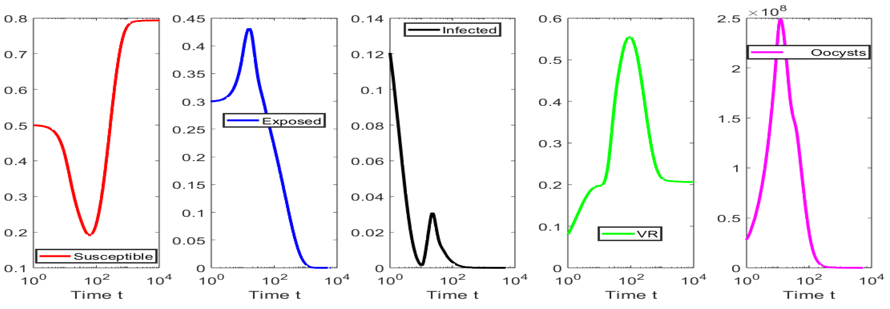
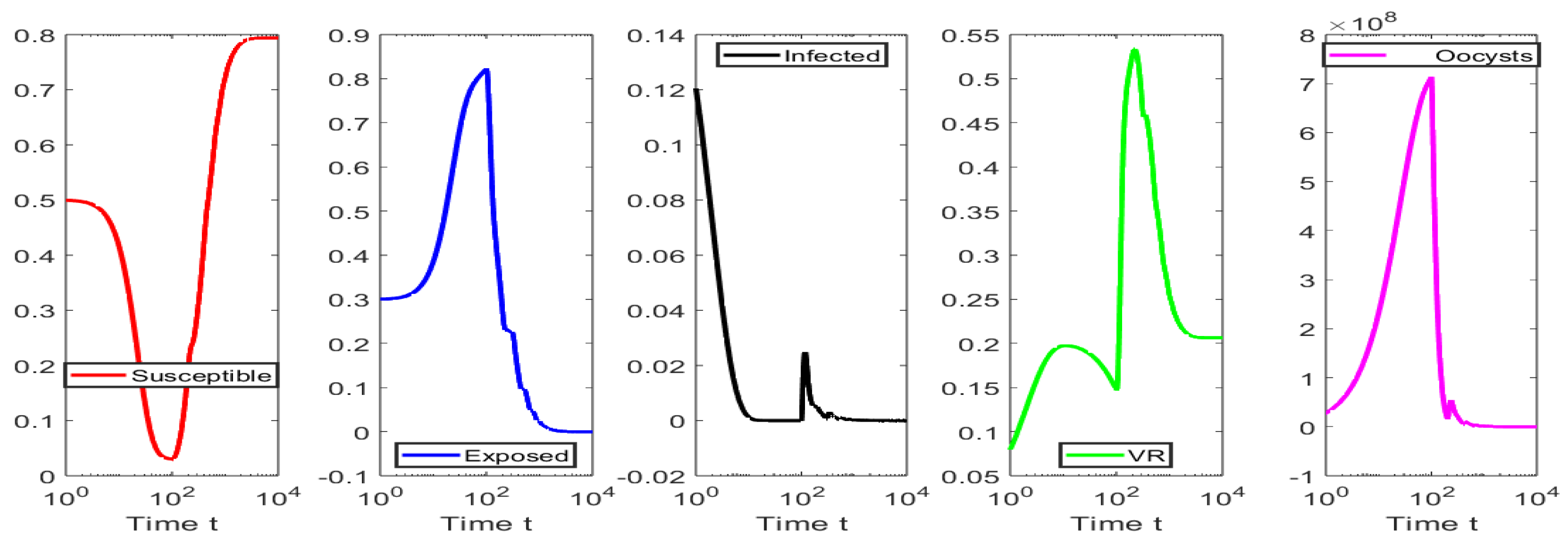
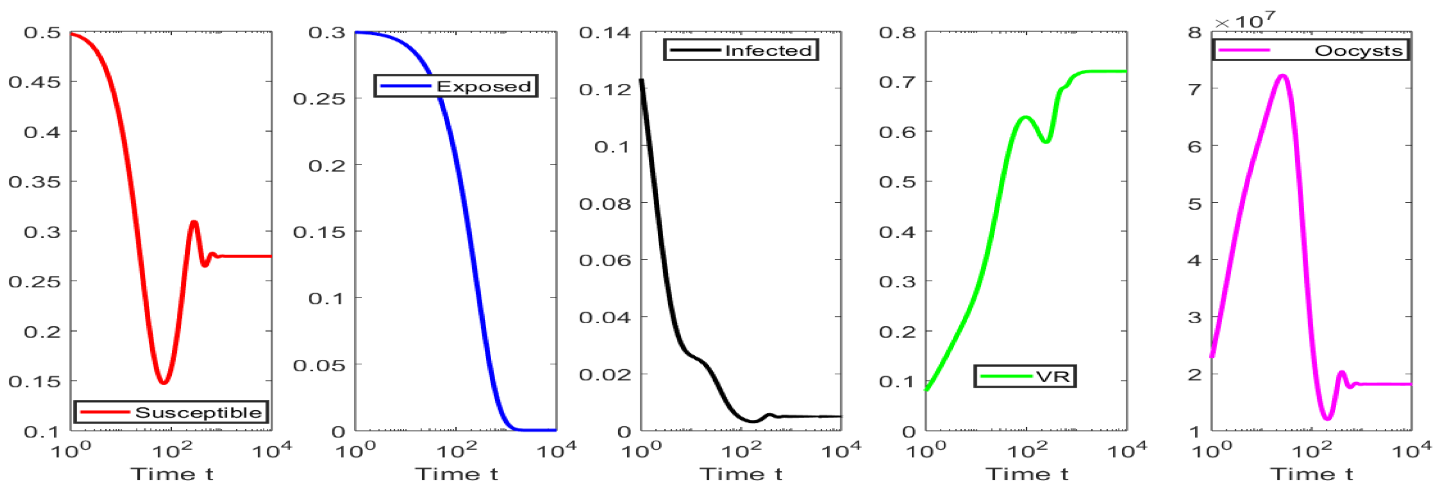
4. Numerical Simulations

In order to investigate the dynamics of toxoplasmosis and corroborate the theoretical findings from the preceding sections, we undertook a range of in silico simulations of mathematical model (1). For the purpose of acquiring distinct values for R 0 d and R 0 , we investigated a range of scenarios with a variety of values for the time delays and the parameters. In particular, we were interested in the values R 0 d > 1 and R 0 d < 1 since these are the threshold values for the long-term behavior of the toxoplasmosis disease. The in silico simulations provide further insights, such as into the transient and long-term behavior of the toxoplasmosis disease in the cat population and the oocyst population. We varied the values of the transmission rate and infectivity of the oocysts. Thus, we could study different scenarios related to the dynamics.
We relied on the Matlab built-in function dde23 to compute the numerical solutions to the delay differential equations [77,114]. For the in silico simulations, we used the values presented in Table 1. The initial conditions were varied in order to obtain a more robust support for the theoretical results. In addition, the equilibrium points were computed for each scenario using the numerical simulations and we contrasted them with the theoretical ones.

4.1. Numerical Simulations for the Scenarios When R 0 d < 1

Here, we describe the in silico simulations where the basic reproduction number R 0 d < 1 and both time delays ( τ 1 and τ 2 ) were different from zero. We used the following initial condition: S ( 0 ) = 0.5 , E ( 0 ) = 0.3 , I ( 0 ) = 0.2 , V R ( 0 ) = 0 , and O ( 0 ) = 1 . Figure 2 shows that the system reached the toxoplasmosis-free equilibrium F * . In this case, we have that R 0 > 1 , but as can be seen, the crucial parameter is R 0 d . It is important to mention that when there are no time delays one obtains that R 0 d = R 0 . Thus, it is possible that, for the toxoplasmosis model without time delays, the disease can be prevalent, but when time delays are taken into account, the disease is eradicated. This has a relevant impact from a public health point of view, since it shows the relevance of the time delays in the dynamics of toxoplasmosis. Figure 3 shows the same scenario but using much larger time delays ( τ 1 = 10 and τ 2 = 10 ). Again, the system reached the toxoplasmosis-free equilibrium F * since R 0 d < 1 . Notice that the increase in the time delays did not affect the value of F * . Finally, we increased the time delays to much larger values to show that long-term behavior would be maintained despite R 0 d being significantly lower. This can be observed in Figure 4.

4.2. Numerical Simulations for the Scenarios When R 0 d > 1

Here, we describe the simulations performed where the basic reproduction number R 0 d > 1 and both time delays ( τ 1 and τ 2 ) were different from zero. Figure 5 shows that the system reached the toxoplasmosis-endemic equilibrium E P * . We increased the transmission rate β in order to have R 0 d > 1 . The system must approach the endemic steady state E P * in accordance with the theoretical results. This section’s second numerical simulation took a greater transmission rate β into account. Again, as Figure 6 shows, the system reached the toxoplasmosis-endemic equilibrium E P * but with larger populations of infected cats and oocysts. This was expected since the toxoplasmosis-endemic equilibrium E P * depends on the time delay β (see Equation (6)). Moreover, the theoretical toxoplasmosis-endemic equilibrium E P * agreed with the numerical endemic equilibrium. The next simulation considered very large time delays to study the possibility of the system losing stability. The results from the previous section suggest that this is not feasible from a mathematical theoretical viewpoint. Figure 7 shows that the system still reached the toxoplasmosis-endemic equilibrium E P * but with larger populations of infected cats and oocysts due to the large transmission rate. It is important to mention that, for many models based on delay differential equations, large time delays can give conditions such that periodic solutions arise. This is an important aspect to consider since, instead of having a steady state, oscillatory behavior could be obtained. It is important to understand this situation from an ecological viewpoint since incorrect public health interventions can be implemented. However, the numerical simulations from this section and the results from the previous section suggest that the mathematical model from Equation (1) cannot have periodic solutions, even for very large time delays. We tested further time delays, such as τ 1 > 1 × 10 3 and τ 2 > 1 × 10 3 . Although those numerical results are not shown here, they were in good agreement with the previous results.

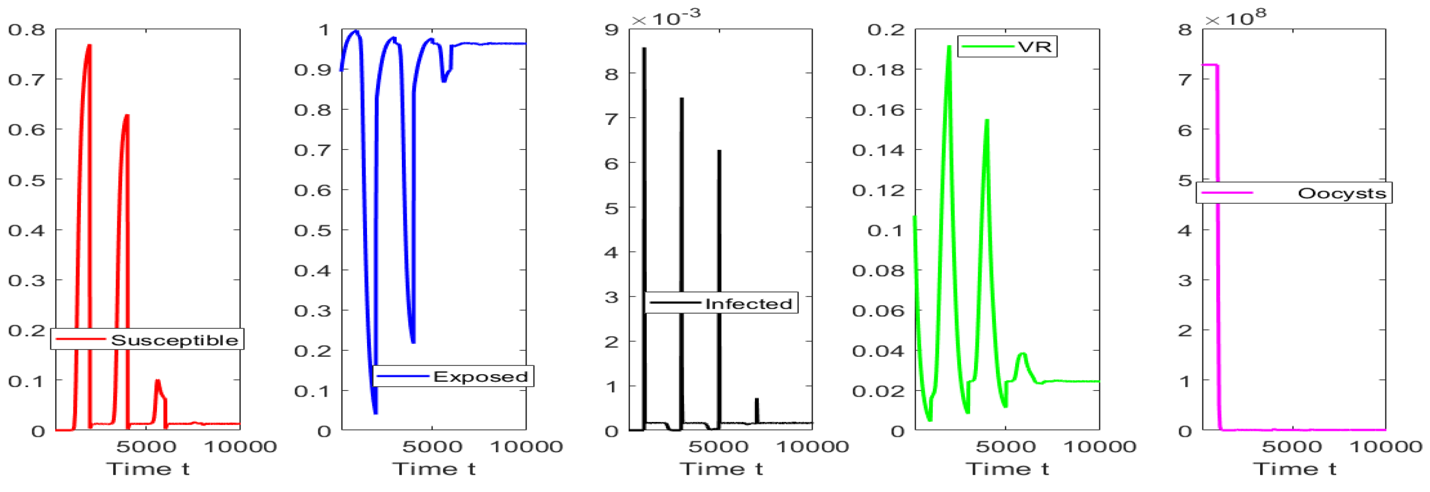
4.3. Numerical Tests for Hopf Bifurcation When R 0 d > 1

Here, we show that, for a set of parameter values that are similar to the previous numerical simulations, the inequality (27) is not satisfied. Therefore, a Hopf bifurcation cannot occur for the set of parameter values that we chose. Let us first rewrite Equation (27) as
| P 0 | 2 + | P 1 | 2 | P 2 | 2 | P 3 | 2 2 A 1 2 + B 1 2 0 .
If we vary ω , we can compute the values of the left-hand side of the inequality (28). Figure 8 shows these values for a large range of values for ω . We use the log scale for the values of the left-hand side of the inequality (28) and, as can be seen, the inequality (28) is not satisfied. It is important to point out that this numerical procedure is not a proof since there are infinitely many potential values for the parameters of model (1). However, these results and the previous numerical simulations suggest that a Hopf bifurcation cannot occur.

5. Conclusions

In order to explore the dynamics of toxoplasmosis, we designed a more realistic mathematical model in this work. The model considers two discrete time delays: the first time delay τ 1 is related to the time it takes the susceptible cats to become infected after effective contact with an oocyst and the second time delay τ 2 is the time that elapses between when the oocysts become present in the environment and when they are able to infect. The main achievement was finding the conditions under which the toxoplasmosis can disappear from the cat population. This can only occur if there are no oocysts in the environment. We also found conditions where the toxoplasmosis became endemic. In addition, we investigated the impact of the two time delays on the toxoplasmosis dynamics. Using dynamical systems theory, we were able to find the basic reproduction number R 0 d for the delay model, which differed from that for the model without delays. We demonstrated that it is a threshold that determines the global long-term dynamics of the toxoplasmosis. We proved that, if R 0 d < 1 , the toxoplasmosis would be eradicated and the toxoplasmosis-free equilibrium would be globally stable. On the other hand, we proved that, if the threshold parameter R 0 d is greater than one, then there is only one toxoplasmosis-endemic equilibrium point. We obtained partial theoretical results and performed numerical simulations that suggested that, if R 0 d > 1 , then the toxoplasmosis-endemic equilibrium point is globally stable. This is a crucial result since it means that, if the basic reproduction number R 0 d is greater than one, the system goes exactly to the toxoplasmosis-endemic steady state. Thus, a globally attractive toxoplasmosis-endemic equilibrium exists regardless of the time delay. Additional numerical simulations were performed and supported the theoretical stability results.
The results obtained in this paper allow us to discuss further the effect of vaccination programs on toxoplasmosis under a more realistic scenario. We provided mathematical analysis that is valid with any parameter values. It is important to mention that, in reality, the values of the parameters have uncertainty, as is common in biology, epidemiology, and public health. The proposed model can be calibrated to real data if we have enough data for some state variables, such as the number of infected cats and the density of oocysts in the environment. This calibration is possible since some values of the parameters are known approximately. However, the uniqueness of the calibration would require identifiability analysis [117,118]. Another aspect that we would like to point out is that the temperature impacts the time delays related to the infectiousness of the oocysts [57]. Therefore, due to climate change, the time delays may be modified in the future. In summary, this study provides further insight into toxoplasmosis dynamics. However, there are still a great number of open problems where even more realistic facts can be included in the mathematical models. For instance, including intermediate hosts, such as mice, would be an important aspect. This is one of the limitations of this work. As with any mathematical model related to biological processes, there are some limitations related to the complex real world. The developed model does not consider humans, who, in a very complex process, might affect the toxoplasmosis dynamics. The model also includes homogeneous mixing, which might not be suitable for some scenarios. Finally, future works that include additional intermediate hosts or new time delays, although challenging, could be useful.

Author Contributions

Methodology, S.S., G.G.-P. and A.J.A.; Software, S.S. and G.G.-P.; Validation, S.S., G.G.-P. and A.J.A.; Formal analysis, S.S. and A.J.A.; Investigation, S.S., G.G.-P. and A.J.A.; Writing—original draft, S.S., G.G.-P. and A.J.A.; Writing—review & editing, S.S. and G.G.-P.; Supervision, G.G.-P. All authors have read and agreed to the published version of the manuscript.

Funding

This research received no external funding.

Data Availability Statement

Data is contained within the article.

Acknowledgments

The authors are grateful to the reviewers for their careful reading of this manuscript and their useful comments to improve the content of this paper. The last author thanks the University of Córdoba, Colombia for the time provided to carry out this research.

Conflicts of Interest

The authors declare no conflict of interest.

References

  1. Attias, M.; Teixeira, D.E.; Benchimol, M.; Vommaro, R.C.; Crepaldi, P.H.; De Souza, W. The life-cycle of Toxoplasma gondii reviewed using animations. Parasites Vectors 2020, 13, 588. [Google Scholar] [CrossRef] [PubMed]
  2. Dubey, J. Advances in the life cycle of Toxoplasma gondii. Int. J. Parasitol. 1998, 28, 1019–1024. [Google Scholar] [CrossRef] [PubMed] [Green Version]
  3. Thomas, F.; Lafferty, K.D.; Brodeur, J.; Elguero, E.; Gauthier-Clerc, M.; Missé, D. Incidence of adult brain cancers is higher in countries where the protozoan parasite Toxoplasma gondii is common. Biol. Lett. 2012, 8, 101–103. [Google Scholar] [CrossRef] [PubMed] [Green Version]
  4. Dubey, J.P. Outbreaks of clinical toxoplasmosis in humans: Five decades of personal experience, perspectives and lessons learned. Parasites Vectors 2021, 14, 263. [Google Scholar] [CrossRef]
  5. McLeod, R.; Cohen, W.; Dovgin, S.; Finkelstein, L.; Boyer, K.M. Human toxoplasma infection. In Toxoplasma gondii; Elsevier: Amsterdam, The Netherlands, 2020; pp. 117–227. [Google Scholar]
  6. Dubey, J. History of the discovery of the life cycle of Toxoplasma gondii. Int. J. Parasitol. 2009, 39, 877–882. [Google Scholar] [CrossRef] [PubMed]
  7. Gilbert, R.E.; Stanford, M.R. Is ocular toxoplasmosis caused by prenatal or postnatal infection? Br. J. Ophthalmol. 2000, 84, 224–226. [Google Scholar] [CrossRef] [Green Version]
  8. Gonzalez, A.J.C.; Matos, I.V.; Revoredo, V.M. Acute toxoplasmosis complicated with myopericarditis and possible encephalitis in an immunocompetent patient. IDCases 2020, 20, e00772. [Google Scholar] [CrossRef]
  9. Alvarado-Esquivel, C.; Estrada-Martínez, S.; Pérez-Álamos, A.R.; Ramos-Nevárez, A.; Botello-Calderón, K.; Alvarado-Félix, Á.O.; Vaquera-Enríquez, R.; Alvarado-Félix, G.A.; Sifuentes-Álvarez, A.; Guido-Arreola, C.A.; et al. Toxoplasma gondii infection and insomnia: A case control seroprevalence study. PLoS ONE 2022, 17, e0266214. [Google Scholar] [CrossRef]
  10. Alvarado-Esquivel, C.; Estrada-Martínez, S.; Ramos-Nevárez, A.; Pérez-Álamos, A.R.; Beristain-García, I.; Alvarado-Félix, Á.O.; Cerrillo-Soto, S.M.; Sifuentes-Álvarez, A.; Alvarado-Félix, G.A.; Guido-Arreola, C.A.; et al. Association between Toxoplasma gondii exposure and suicidal behavior in patients attending primary health care clinics. Pathogens 2021, 10, 677. [Google Scholar] [CrossRef]
  11. Hosseininejad, Z.; Sharif, M.; Sarvi, S.; Amouei, A.; Hosseini, S.A.; Nayeri Chegeni, T.; Anvari, D.; Saberi, R.; Gohardehi, S.; Mizani, A.; et al. Toxoplasmosis seroprevalence in rheumatoid arthritis patients: A systematic review and meta-analysis. PLoS Neglect. Trop. Dis. 2018, 12, e0006545. [Google Scholar] [CrossRef]
  12. Beshay, E.V.N.; El-Refai, S.A.; Helwa, M.A.; Atia, A.F.; Dawoud, M.M. Toxoplasma gondii as a possible causative pathogen of type-1 diabetes mellitus: Evidence from case-control and experimental studies. Exp. Parasitol. 2018, 188, 93–101. [Google Scholar] [CrossRef] [PubMed]
  13. De Haan, L.; Sutterland, A.L.; Schotborgh, J.V.; Schirmbeck, F.; de Haan, L. Association of Toxoplasma gondii seropositivity with cognitive function in healthy people: A systematic review and meta-analysis. JAMA Psychiatry 2021, 78, 1103–1112. [Google Scholar] [CrossRef]
  14. Caldrer, S.; Vola, A.; Ferrari, G.; Ursini, T.; Mazzi, C.; Meroni, V.; Beltrame, A. Toxoplasma gondii Serotypes in Italian and Foreign Populations: A Cross-Sectional Study Using a Homemade ELISA Test. Microorganisms 2022, 10, 1577. [Google Scholar] [CrossRef] [PubMed]
  15. Fernández-Escobar, M.; Schares, G.; Maksimov, P.; Joeres, M.; Ortega-Mora, L.M.; Calero-Bernal, R. Toxoplasma gondii Genotyping: A Closer Look Into Europe. Front. Cell. Infect. Microbiol. 2022, 12, 842595. [Google Scholar] [CrossRef]
  16. Galal, L.; Hamidović, A.; Dardé, M.L.; Mercier, M. Diversity of Toxoplasma gondii strains at the global level and its determinants. Food Waterborne Parasitol. 2019, 15, e00052. [Google Scholar] [CrossRef] [PubMed]
  17. CDC. Center for Disease Control and Prevention, Toxoplasmosis. Available online: https://www.cdc.gov/parasites/toxoplasmosis/ (accessed on 1 May 2021).
  18. Morris, J.G., Jr.; Havelaar, A. Toxoplasma gondii. In Foodborne Infections and Intoxications; Elsevier: Amsterdam, The Netherlands, 2021; pp. 347–361. [Google Scholar]
  19. Zhu, S.; VanWormer, E.; Martínez-López, B.; Bahia-Oliveira, L.M.G.; DaMatta, R.A.; Rodrigues, P.S.; Shapiro, K. Quantitative Risk Assessment of Oocyst Versus Bradyzoite Foodborne Transmission of Toxoplasma gondii in Brazil. Pathogens 2023, 12, 870. [Google Scholar] [CrossRef] [PubMed]
  20. Dubey, J.P. The history of Toxoplasma gondii—The first 100 years. J. Eukaryot. Microbiol. 2008, 55, 467–475. [Google Scholar] [CrossRef]
  21. Havelaar, A.H.; Kirk, M.D.; Torgerson, P.R.; Gibb, H.J.; Hald, T.; Lake, R.J.; Praet, N.; Bellinger, D.C.; De Silva, N.R.; Gargouri, N.; et al. World Health Organization global estimates and regional comparisons of the burden of foodborne disease in 2010. PLoS Med. 2015, 12, e1001923. [Google Scholar] [CrossRef] [Green Version]
  22. Opsteegh, M.; Kortbeek, T.M.; Havelaar, A.H.; van der Giessen, J.W. Intervention strategies to reduce human Toxoplasma gondii disease burden. Clin. Infect. Dis. 2015, 60, 101–107. [Google Scholar] [CrossRef] [Green Version]
  23. Torgerson, P.R.; Mastroiacovo, P. The global burden of congenital toxoplasmosis: A systematic review. Bull. World Health Organ. 2013, 91, 501–508. [Google Scholar] [CrossRef]
  24. Scallan, E.; Hoekstra, R.M.; Angulo, F.J.; Tauxe, R.V.; Widdowson, M.A.; Roy, S.L.; Jones, J.L.; Griffin, P.M. Foodborne illness acquired in the United States—Major pathogens. Emerg. Infect. Dis. 2011, 17, 7–15. [Google Scholar] [CrossRef] [PubMed]
  25. Batz, M.B.; Hoffmann, S.; Morris, J.G., Jr. Ranking the disease burden of 14 pathogens in food sources in the United States using attribution data from outbreak investigations and expert elicitation. J. Food Prot. 2012, 75, 1278–1291. [Google Scholar] [CrossRef] [Green Version]
  26. Deng, H.; Cummins, R.; Schares, G.; Trevisan, C.; Enemark, H.; Waap, H.; Srbljanovic, J.; Djurkovic-Djakovic, O.; Pires, S.M.; van der Giessen, J.W.; et al. Mathematical modelling of Toxoplasma gondii transmission: A systematic review. Food Waterborne Parasitol. 2021, 22, e00102. [Google Scholar] [CrossRef]
  27. Aramini, J.; Stephen, C.; Dubey, J.P.; Engelstoft, C.; Schwantje, H.; Ribble, C.S. Potential contamination of drinking water with Toxoplasma gondii oocysts. Epidemiol. Infect. Camb. Univ. Press 1999, 122, 305–315. [Google Scholar] [CrossRef] [PubMed]
  28. Hill, D.; Dubey, J. Toxoplasma gondii: Transmission, diagnosis and prevention. Clin. Microbiol. Infect. 2002, 8, 634–640. [Google Scholar] [CrossRef] [Green Version]
  29. Frenkel, J.; Ruiz, A.; Chinchilla, M. Soil survival of Toxoplasma oocysts in Kansas and Costa Rica. Am. J. Trop. Med. Hyg. 1975, 24, 439–443. [Google Scholar] [CrossRef]
  30. Kuruca, L.; Belluco, S.; Vieira-Pinto, M.; Antic, D.; Blagojevic, B. Current control options and a way towards risk-based control of Toxoplasma gondii in the meat chain. Food Control 2023, 146, 109556. [Google Scholar] [CrossRef]
  31. Fayer, R. Toxoplasmosis update and public health implications. Can. Vet. J. 1981, 22, 344–352. [Google Scholar]
  32. Innes, E.A.; Hamilton, C.; Garcia, J.L.; Chryssafidis, A.; Smith, D. A one health approach to vaccines against Toxoplasma gondii. Food Waterborne Parasitol. 2019, 15, e00053. [Google Scholar] [CrossRef] [PubMed]
  33. Marinović, A.A.B.; Opsteegh, M.; Deng, H.; Suijkerbuijk, A.W.; van Gils, P.F.; Van Der Giessen, J. Prospects of toxoplasmosis control by cat vaccination. Epidemics 2020, 30, 100380. [Google Scholar] [CrossRef]
  34. Smith, N.C.; Goulart, C.; Hayward, J.A.; Kupz, A.; Miller, C.M.; van Dooren, G.C. Control of human toxoplasmosis. Int. J. Parasitol. 2021, 51, 95–121. [Google Scholar] [CrossRef] [PubMed]
  35. Wolf, P.J.; Hamilton, F. Managing free-roaming cats in US cities: An object lesson in public policy and citizen action. J. Urban Aff. 2020, 44, 221–242. [Google Scholar] [CrossRef]
  36. Dubey, J. A review of Toxoplasmosis in cattle. Vet. Parasitol. 1986, 22, 177–202. [Google Scholar] [CrossRef]
  37. Dubey, J. A review of Toxoplasmosis in pigs. Vet. Parasitol. 1986, 19, 181–223. [Google Scholar] [CrossRef] [PubMed]
  38. Dubey, J.; Beattie, C. Toxoplasmosis of Animals and Man; CRC Press: Boca Raton, FL, USA, 1988. [Google Scholar]
  39. Dubey, J.P. Strategies to reduce transmission of Toxoplasma gondii to animals and humans. Vet. Parasitol. 1996, 64, 65–70. [Google Scholar] [CrossRef]
  40. Dubey, J.; Mattix, M.; Lipscomb, T. Lesions of neonatally induced toxoplasmosis in cats. Vet. Pathol. 1996, 33, 290–295. [Google Scholar] [CrossRef] [PubMed]
  41. Williams, R.; Morley, E.; Hughes, J.; Duncanson, P.; Terry, R.; Smith, J.; Hide, G. High levels of congenital transmission of Toxoplasma gondii in longitudinal and cross-sectional studies on sheep farms provides evidence of vertical transmission in ovine hosts. Parasitology 2005, 130, 301–307. [Google Scholar] [CrossRef] [Green Version]
  42. Sacks, J.J.; Roberto, R.R.; Brooks, N.F. Toxoplasmosis infection associated with raw goat’s milk. JAMA 1982, 248, 1728–1732. [Google Scholar] [CrossRef]
  43. Simon, J.A.; Pradel, R.; Aubert, D.; Geers, R.; Villena, I.; Poulle, M.L. A multi-event capture-recapture analysis of Toxoplasma gondii seroconversion dynamics in farm cats. Parasites Vectors 2018, 11, 339. [Google Scholar] [CrossRef]
  44. Webster, J.P. The effect of Toxoplasma gondii on animal behavior: Playing cat and mouse. Schizophr. Bull. 2007, 33, 752–756. [Google Scholar] [CrossRef]
  45. Dabritz, H.; Conrad, P.A. Cats and Toxoplasma: Implications for public health. Zoonoses Public Health 2010, 57, 34–52. [Google Scholar] [CrossRef] [PubMed]
  46. Murphy, R.G.; Williams, R.H.; Hughes, J.M.; Hide, G.; Ford, N.J.; Oldbury, D.J. The urban house mouse (Mus domesticus) as a reservoir of infection for the human parasite Toxoplasma gondii: An unrecognised public health issue? Int. J. Environ. Health Res. 2008, 18, 177–185. [Google Scholar] [CrossRef]
  47. Arenas, A.J.; González-Parra, G.; Micó, R.J.V. Modeling toxoplasmosis spread in cat populations under vaccination. Theor. Popul. Biol. 2010, 77, 227–237. [Google Scholar] [CrossRef]
  48. Ferreira, J.D.; Echeverry, L.M.; Rincon, C.A.P. Stability and bifurcation in epidemic models describing the transmission of toxoplasmosis in human and cat populations. Math. Methods Appl. Sci. 2017, 40, 5575–5592. [Google Scholar] [CrossRef]
  49. González-Parra, G.C.; Arenas, A.J.; Aranda, D.F.; Villanueva, R.J.; Jódar, L. Dynamics of a model of Toxoplasmosis disease in human and cat populations. Comput. Math. Appl. 2009, 57, 1692–1700. [Google Scholar] [CrossRef] [Green Version]
  50. Turner, M.; Lenhart, S.; Rosenthal, B.; Zhao, X. Modeling effective transmission pathways and control of the world’s most successful parasite. Theor. Popul. Biol. 2013, 86, 50–61. [Google Scholar] [CrossRef]
  51. Lélu, M.; Langlais, M.; Poulle, M.L.; Gilot-Fromont, E. Transmission dynamics of Toxoplasma gondii along an urban–rural gradient. Theor. Popul. Biol. 2010, 78, 139–147. [Google Scholar] [CrossRef]
  52. González-Parra, G.; Arenas, A.J.; Chen-Charpentier, B.; Sultana, S. Mathematical modeling of toxoplasmosis with multiple hosts, vertical transmission and cat vaccination. Comput. Appl. Math. 2023, 42, 88. [Google Scholar] [CrossRef]
  53. Sultana, S.; González-Parra, G.; Arenas, A.J. A Generalized Mathematical Model of Toxoplasmosis with an Intermediate Host and the Definitive Cat Host. Mathematics 2023, 11, 1642. [Google Scholar] [CrossRef]
  54. Mateus-Pinilla, N.; Hannon, B.; Weigel, R. A computer simulation of the prevention of the transmission of Toxoplasma gondii on swine farms using a feline T. gondii vaccine. Prev. Vet. Med. 2002, 55, 17–36. [Google Scholar] [CrossRef]
  55. Sullivan, A.; Agusto, F.; Bewick, S.; Su, C.; Lenhart, S.; Zhao, X. A mathematical model for within-host Toxoplasma gondii invasion dynamics. Math. Biosci. Eng. 2012, 9, 647. [Google Scholar] [PubMed]
  56. Dubey, J. Duration of Immunity to Shedding of Toxoplasma gondii Oocysts by Cats. J. Parasitol. 1995, 81, 410–415. [Google Scholar] [CrossRef] [PubMed]
  57. Frenkel, J.; Dubey, J.; Miller, N.L. Toxoplasma gondii in cats: Fecal stages identified as coccidian oocysts. Science 1970, 167, 893–896. [Google Scholar] [CrossRef]
  58. Dubey, J.; Lindsay, D.S.; Lappin, M.R. Toxoplasmosis and other intestinal coccidial infections in cats and dogs. Vet. Clin. Small Anim. Pract. 2009, 39, 1009–1034. [Google Scholar] [CrossRef] [PubMed]
  59. Jiang, W.; Sullivan, A.M.; Su, C.; Zhao, X. An agent-based model for the transmission dynamics of Toxoplasma gondii. J. Theor. Biol. 2012, 293, 15–26. [Google Scholar] [CrossRef]
  60. Lappin, M. Feline toxoplasmosis. InPractice 1999, 21, 578–589. [Google Scholar] [CrossRef]
  61. Burrells, A.; Bartley, P.; Zimmer, I.; Roy, S.; Kitchener, A.C.; Meredith, A.; Wright, S.; Innes, E.; Katzer, F. Evidence of the three main clonal Toxoplasma gondii lineages from wild mammalian carnivores in the UK. Parasitology 2013, 140, 1768–1776. [Google Scholar] [CrossRef]
  62. Dardé, M. Toxoplasma gondii “new” genotypes and virulence. Parasite 2008, 15, 366–371. [Google Scholar] [CrossRef] [Green Version]
  63. Lindsay, D.; Dubey, J. Toxoplasma gondii: The changing paradigm of congenital toxoplasmosis. Parasitology 2011, 138, 1829–1831. [Google Scholar] [CrossRef] [Green Version]
  64. Arenas, A.J.; González-Parra, G.; Naranjo, J.J.; Cogollo, M.; De La Espriella, N. Mathematical Analysis and Numerical Solution of a Model of HIV with a Discrete Time Delay. Mathematics 2021, 9, 257. [Google Scholar] [CrossRef]
  65. Chen-Charpentier, B.M.; Jackson, M. Direct and indirect optimal control applied to plant virus propagation with seasonality and delays. J. Comput. Appl. Math. 2020, 380, 112983. [Google Scholar] [CrossRef]
  66. Smith, H.L. An Introduction to Delay Differential Equations with Applications to the Life Sciences; Springer: Berlin/Heidelberg, Germany, 2011; Volume 57. [Google Scholar]
  67. Rihan, F.A. Delay Differential Equations and Applications to Biology; Springer: Berlin/Heidelberg, Germany, 2021. [Google Scholar]
  68. Hethcote, H. Mathematics of infectious diseases. SIAM Rev. 2005, 42, 599–653. [Google Scholar] [CrossRef] [Green Version]
  69. Xu, R. Global dynamics of an {SEIS} epidemiological model with time delay describing a latent period. Math. Comput. Simul. 2012, 85, 90–102. [Google Scholar] [CrossRef]
  70. Yan, P.; Liu, S. SEIR epidemic model with delay. ANZIAM J. 2006, 48, 119–134. [Google Scholar] [CrossRef] [Green Version]
  71. Guo, B.Z.; Cai, L.M. A note for the global stability of a delay differential equation of hepatitis B virus infection. Math. Biosci. Eng. 2011, 8, 689–694. [Google Scholar]
  72. Samanta, G.P. Dynamic behaviour for a nonautonomous heroin epidemic model with time delay. J. Appl. Math. Comput. 2011, 35, 161–178. [Google Scholar] [CrossRef]
  73. Nelson, P.W.; Murray, J.D.; Perelson, A.S. A model of HIV-1 pathogenesis that includes an intracellular delay. Math. Biosci. 2000, 163, 201–215. [Google Scholar] [CrossRef] [PubMed]
  74. Castro, M.Á.; García, M.A.; Martín, J.A.; Rodríguez, F. Exact and nonstandard finite difference schemes for coupled linear delay differential systems. Mathematics 2019, 7, 1038. [Google Scholar] [CrossRef] [Green Version]
  75. García, M.; Castro, M.; Martín, J.A.; Rodríguez, F. Exact and nonstandard numerical schemes for linear delay differential models. Appl. Math. Comput. 2018, 338, 337–345. [Google Scholar] [CrossRef]
  76. Kerr, G.; González-Parra, G.; Sherman, M. A new method based on the Laplace transform and Fourier series for solving linear neutral delay differential equations. Appl. Math. Comput. 2022, 420, 126914. [Google Scholar] [CrossRef]
  77. Shampine, L.F.; Thompson, S. Numerical solution of delay differential equations. In Delay Differential Equations; Springer: Berlin/Heidelberg, Germany, 2009; pp. 1–27. [Google Scholar]
  78. Bachar, M. On periodic solutions of delay differential equations with impulses. Symmetry 2019, 11, 523. [Google Scholar] [CrossRef] [Green Version]
  79. Bartłomiejczyk, A.; Bodnar, M. Hopf bifurcation in time-delayed gene expression model with dimers. Math. Methods Appl. Sci. 2023, 46, 12087–12111. [Google Scholar] [CrossRef]
  80. Gökçe, A. A dynamic interplay between Allee effect and time delay in a mathematical model with weakening memory. Appl. Math. Comput. 2022, 430, 127306. [Google Scholar] [CrossRef]
  81. Liu, Y.; Cai, J.; Xu, H.; Shan, M.; Gao, Q. Stability and Hopf bifurcation of a love model with two delays. Math. Comput. Simul. 2023, 205, 558–580. [Google Scholar] [CrossRef]
  82. Maji, C.; Al Basir, F.; Mukherjee, D.; Ravichandran, C.; Nisar, K. COVID-19 propagation and the usefulness of awareness-based control measures: A mathematical model with delay. AIMS Math 2022, 7, 12091–12105. [Google Scholar] [CrossRef]
  83. Najm, F.; Yafia, R.; Aziz-Alaoui, M. Hopf Bifurcation in Oncolytic Therapeutic Modeling: Viruses as Anti-Tumor Means with Viral Lytic Cycle. Int. J. Bifurc. Chaos 2022, 32, 2250171. [Google Scholar] [CrossRef]
  84. Ruschel, S.; Pereira, T.; Yanchuk, S.; Young, L.S. An SIQ delay differential equations model for disease control via isolation. J. Math. Biol. 2019, 79, 249–279. [Google Scholar] [CrossRef] [Green Version]
  85. Sepulveda, G.; Arenas, A.J.; González-Parra, G. Mathematical Modeling of COVID-19 Dynamics under Two Vaccination Doses and Delay Effects. Mathematics 2023, 11, 369. [Google Scholar] [CrossRef]
  86. Achouri, H.; Aouiti, C. Bogdanov–Takens and triple zero bifurcations for a neutral functional differential equations with multiple delays. J. Dyn. Differ. Equ. 2021, 35, 355–380. [Google Scholar] [CrossRef]
  87. Angelova, M.; Shelyag, S. Delay-differential equations for glucose-insulin regulation. In 2019–20 MATRIX Annals; Springer: Berlin/Heidelberg, Germany, 2021; pp. 299–306. [Google Scholar]
  88. Diekmann, O.; Van Gils, S.A.; Lunel, S.M.; Walther, H.O. Delay Equations: Functional-, Complex-, and Nonlinear Analysis; Springer Science & Business Media: Berlin/Heidelberg, Germany, 2012; Volume 110. [Google Scholar]
  89. Masood, F.; Moaaz, O.; Askar, S.S.; Alshamrani, A. New Conditions for Testing the Asymptotic Behavior of Solutions of Odd-Order Neutral Differential Equations with Multiple Delays. Axioms 2023, 12, 658. [Google Scholar] [CrossRef]
  90. Pospíšil, M. Representation of solutions of systems of linear differential equations with multiple delays and nonpermutable variable coefficients. Math. Model. Anal. 2020, 25, 303–322. [Google Scholar] [CrossRef] [Green Version]
  91. Santra, S.S.; Bazighifan, O.; Ahmad, H.; Yao, S.W. Second-order differential equation with multiple delays: Oscillation theorems and applications. Complexity 2020, 2020, 8853745. [Google Scholar] [CrossRef]
  92. Ge, J.; Xu, J. An analytical method for studying double Hopf bifurcations induced by two delays in nonlinear differential systems. Sci. China Technol. Sci. 2020, 63, 597–602. [Google Scholar] [CrossRef]
  93. Lin, X.; Wang, H. Stability analysis of delay differential equations with two discrete delays. Can. Appl. Math. Q. 2012, 20, 519–533. [Google Scholar]
  94. Pal, S.; Gupta, A.; Misra, A.K.; Dubey, B. Chaotic dynamics of a stage-structured prey-predator system with hunting cooperation and fear in presence of two discrete time delays. J. Biol. Syst. 2023, 31, 611–642. [Google Scholar] [CrossRef]
  95. Cheng, Z.; Song, Q.; Xiao, M. Bifurcation and control of disease spreading networks model with two delays. Asian J. Control 2023, 25, 1323–1335. [Google Scholar] [CrossRef]
  96. Gu, K.; Niculescu, S.I.; Chen, J. On stability crossing curves for general systems with two delays. J. Math. Anal. Appl. 2005, 311, 231–253. [Google Scholar] [CrossRef] [Green Version]
  97. Gao, S.; Chen, L.; Teng, Z. Pulse vaccination of an SEIR epidemic model with time delay. Nonlinear Anal. Real World Appl. 2008, 9, 599–607. [Google Scholar] [CrossRef]
  98. Sykes, D.; Rychtář, J. A game-theoretic approach to valuating toxoplasmosis vaccination strategies. Theor. Popul. Biol. 2015, 105, 33–38. [Google Scholar] [CrossRef]
  99. Freyre, A.; Choromanski, L.; Fishback, J.; Popiel, I. Immunization of cats with tissue cysts, bradyzoites, and tachyzoites of the T-263 strain of Toxoplasma gondii. J. Parasitol. 1993, 79, 716–719. [Google Scholar] [CrossRef]
  100. Frenkel, J. Transmission of toxoplasmosis and the role of immunity in limiting transmission and illness. J. Am. Vet. Med. Assoc. 1990, 196, 233–240. [Google Scholar] [PubMed]
  101. Powell, C.C.; Lappin, M.R. Clinical ocular toxoplasmosis in neonatal kittens. Vet. Ophthalmol. 2001, 4, 87–92. [Google Scholar] [CrossRef] [PubMed]
  102. Sato, K.; Iwamoto, I.; Yoshiki, K. Experimental toxoplasmosis in pregnant cats. Vet. Ophthalmol. 1993, 55, 1005–1009. [Google Scholar] [CrossRef] [Green Version]
  103. Dubey, J.; Lappin, M.; Thulliez, P. Diagnosis of induced toxoplasmosis in neonatal cats. J. Am. Vet. Med. Assoc. 1995, 207, 179–185. [Google Scholar] [PubMed]
  104. Powell, C.C.; Brewer, M.; Lappin, M.R. Detection of Toxoplasma gondii in the milk of experimentally infected lactating cats. Vet. Parasitol. 2001, 102, 29–33. [Google Scholar] [CrossRef] [PubMed]
  105. Kuang, Y. Delay Differential Equations: With Applications in Population Dynamics; Academic Press: Cambridge, MA, USA, 1993. [Google Scholar]
  106. Gourley, S.A.; Kuang, Y.; Nagy, J.D. Dynamics of a delay differential equation model of hepatitis B virus infection. J. Biol. Dyn. 2008, 2, 140–153. [Google Scholar] [CrossRef] [Green Version]
  107. Jack, K.; Hale, S.M.V.L. Introduction to Functional Differential Equations, 1st ed.; Applied Mathematical Sciences 99; Springer: Berlin/Heidelberg, Germany, 1993. [Google Scholar]
  108. Hale, J. Ordinary Differential Equations; Wiley: New York, NY, USA, 1969. [Google Scholar]
  109. Hirsh, M.; Smale, S.; Devaney, R.L. Differential Equations, Dynamical Systems and an Introduction to Chaos; Academic Press: Cambridge, MA, USA, 2004. [Google Scholar]
  110. Murray, J.D. Mathematical Biology I. An Introduction; Springer: Berlin/Heidelberg, Germany, 2002. [Google Scholar]
  111. González-Parra, G.; Sultana, S.; Arenas, A.J. Mathematical modeling of toxoplasmosis considering a time delay in the infectivity of oocysts. Mathematics 2022, 10, 354. [Google Scholar] [CrossRef]
  112. Sultana, S.; González-Parra, G.; Arenas, A.J. Dynamics of toxoplasmosis in the cat’s population with an exposed stage and a time delay. Math. Biosci. Eng. 2022, 19, 12655–12676. [Google Scholar] [CrossRef]
  113. La Salle, J.P. The Stability of Dynamical Systems; SIAM: Philadelphia, PA, USA, 1976. [Google Scholar]
  114. Shampine, L.F.; Thompson, S. Solving ddes in matlab. Appl. Numer. Math. 2001, 37, 441–458. [Google Scholar] [CrossRef]
  115. Berthier, K.; Langlais, M.; Auger, P.; Pontier, D. Dynamics of a feline virus with two transmission modes within exponentially growing host populations. Proc. R. Soc. B Biol. Sci. 2000, 267, 2049–2056. [Google Scholar] [CrossRef]
  116. Fayer, R. Toxoplasma gondii: Transmission, diagnosis and prevention. Can. Vet. 1981, 22, 344–352. [Google Scholar]
  117. Raue, A.; Kreutz, C.; Maiwald, T.; Bachmann, J.; Schilling, M.; Klingmüller, U.; Timmer, J. Structural and practical identifiability analysis of partially observed dynamical models by exploiting the profile likelihood. Bioinformatics 2009, 25, 1923–1929. [Google Scholar] [CrossRef] [PubMed] [Green Version]
  118. González-Parra, G.; Díaz-Rodríguez, M.; Arenas, A.J. Mathematical modeling to study the impact of immigration on the dynamics of the COVID-19 pandemic: A case study for Venezuela. Spat. Spatio-Temp. Epidemiol. 2022, 43, 100532. [Google Scholar] [CrossRef] [PubMed]
Figure 1. Graphical representation of mathematical model (1) with two time delays τ 1 and τ 2 .
Mathematics 11 03463 g001
Figure 2. Dynamic behavior of the subpopulations when β = 0.17309 × 10 9 and γ = 0.001 . The components of the toxoplasmosis-free equilibrium point are S * 0.793 , I * = 0 , and O * = 0 . The initial state is S ( 0 ) = 0.5 , I ( 0 ) = 0.3 , and O ( 0 ) = 300 . The basic reproduction numbers R 0 d 0.999 and R 0 1.00003 > 1 , and both time delays are different from zero ( τ 1 = 1 and τ 2 = 1 ).
Mathematics 11 03463 g002
Figure 3. Dynamic behavior of the subpopulations when β = 0.17309 × 10 9 and γ = 0.001 . The components of the toxoplasmosis-free equilibrium point are S * 0.793 , I * = 0 , and O * = 0 . The initial state is S ( 0 ) = 0.5 , I ( 0 ) = 0.3 , and O ( 0 ) = 300 . The basic reproduction numbers R 0 d 0.96 and R 0 1.00003 > 1 , and both time delays are different from zero ( τ 1 = 10 and τ 2 = 10 ).
Mathematics 11 03463 g003
Figure 4. Dynamic behavior of the subpopulations when β = 0.17309 × 10 9 and γ = 0.001 . The components of the toxoplasmosis-free equilibrium point are S * 0.793 , I * = 0 , and O * = 0 . The initial state is S ( 0 ) = 0.5 , I ( 0 ) = 0.3 , and O ( 0 ) = 300 . The basic reproduction numbers R 0 d 0.7 and R 0 1.01 > 1 , and both time delays are different from zero ( τ 1 = 100 and τ 2 = 100 ).
Mathematics 11 03463 g004
Figure 5. Dynamic behavior of the subpopulations when β = 0.18 × 10 9 and γ = 0.001 . The components of the toxoplasmosis-endemic equilibrium point are S * 0.76 ,   E * 0.00001 ,   I * 0.0003 , and O * 1.05 × 10 6 . The initial state is S ( 0 ) = 0.5 , I ( 0 ) = 0.3 , and O ( 0 ) = 300 . The basic reproduction numbers R 0 d 1.03 and R 0 1.01 > 1 , and both time delays are different from zero ( τ 1 = 0.1 and τ 2 = 0.1 ).
Mathematics 11 03463 g005
Figure 6. Dynamic behavior of the subpopulations when β = 0.5 × 10 9 and γ = 0.001 . The components of the toxoplasmosis-endemic equilibrium point are S * 0.27 ,   E * 0.00025 ,   I * 0.005 , and O * 1.81 × 10 7 . The initial state is S ( 0 ) = 0.5 , I ( 0 ) = 0.3 , and O ( 0 ) = 300 . The basic reproduction numbers R 0 d 2.88 and R 0 1.69 > 1 , and both time delays are different from zero ( τ 1 = 0.1 and τ 2 = 0.1 ).
Mathematics 11 03463 g006
Figure 7. Dynamic behavior of the subpopulations when β = 0.5 × 10 6 and γ = 0.001 . The components of the toxoplasmosis-endemic equilibrium point are S * 0.0128 ,   E * 0.962 ,   I * 0.00016 , and O * 5.88 × 10 5 . The initial state is S ( 0 ) = 0.5 , I ( 0 ) = 0.3 , and O ( 0 ) = 300 . The basic reproduction numbers R 0 d 61 and R 0 53 , and both time delays are different from zero ( τ 1 = 1 × 10 3 and τ 2 = 1 × 10 3 ).
Mathematics 11 03463 g007
Figure 8. Graph of the values of the left-hand side of the inequality (28) for different values of ω .
Mathematics 11 03463 g008
Table 1. Explanation of the parameters of the delayed model (1) and their values.
ParameterDescriptionValue
μ Birth/death rates (cats) 1 / 260 (1/weeks) [115]
α Shedding period 1 / 2 (1/weeks) [56]
μ 0 Clearance rate 1 / 26 (1/day) [54,56]
kOocysts per day (cat) 20 × 10 6 (1/day) [116]
β Transmission rateVaried
γ Vaccination rateVaried
Disclaimer/Publisher’s Note: The statements, opinions and data contained in all publications are solely those of the individual author(s) and contributor(s) and not of MDPI and/or the editor(s). MDPI and/or the editor(s) disclaim responsibility for any injury to people or property resulting from any ideas, methods, instructions or products referred to in the content.

