Complementary Gamma Zero-Truncated Poisson Distribution and Its Application

Abstract

Numerous lifetime distributions have been developed to assist researchers in various fields. This paper proposes a new continuous three-parameter lifetime distribution called the complementary gamma zero-truncated Poisson distribution (CGZTP), which combines the distribution of the maximum of a series of independently identical gamma-distributed random variables with zero-truncated Poisson random variables. The proposed distribution’s properties, including proofs of the probability density function, cumulative distribution function, survival function, hazard function, and moments, are discussed. The unknown parameters are estimated using the maximum likelihood method, whose asymptotic properties are examined. In addition, Wald confidence intervals are constructed for the CGZTP parameters. Simulation studies are conducted to evaluate the efficacy of parameter estimation, and three real-world data applications demonstrate that CGZTP can be an alternative distribution for fitting data.

1. Introduction

The gamma distribution is widely used in modeling lifetime data. However, the gamma distribution does not provide a reasonable parametric fit for modeling phenomena with non-monotone hazard functions, such as bathtub hazard functions. Some new distributions to model lifetime data have appeared in the recent literature by compounding existing lifetime models with several discrete distributions. For instance, a distribution is obtained by assuming the minimum or maximum of continuous positive random variables. To accomplish this, Adamidis and Loukas [1] proposed an exponential-geometric (EG) distribution by compounding the geometric distribution and the exponential distribution. A complementary version of the EG distribution was proposed by Louzada et al. [2], which would be applied to maximum lifetime data. The Weibull-geometric (WG) distribution with the minimum compounded function was proposed by Barreto-Souza et al. [3], and its maximum version was given by Tojeiro et al. [4]. Zakerzadeh and Mahmoudi [5] introduced a Lindley-geometric (LG) distribution, whereas Gui et al. [6] introduced a complementary Lindley-geometric distribution. In addition, several new compoundings of the Poisson distribution and some lifetime models have been introduced in closed forms, such as Kus [7], who proposed an Exponential-Poisson (EP) distribution, Hemmati et al. [8] and Lu and Shi [9], who proposed a Weibull-Poisson (WP), whose complementary version was given by Ismail [10]. Alkarni and Oraby [11] defined the class of Poisson with some lifetime distributions, and some properties of the Rayleigh-Poisson and Pareto-Poisson distributions are presented in their works. Additionally, Gui et al. [12] proposed a Lindley-Poisson (LP) distribution.

In this article, the gamma and zero-truncated Poisson distributions are compounded to generate a new lifetime distribution using the maximum function, which the hazard function can perform in a bathtub shape. This novel distribution is established as the complementary gamma zero-truncated Poisson distribution (CGZTP). This article is structured as follows: In Section 2, the distribution is mathematically derived, and in Section 3, its important properties are examined. In Section 4 and Section 5, the estimates of the parameters and the results of a simulation study are presented. An application to real datasets is provided in Section 6. Finally, Section 7 concludes the paper.

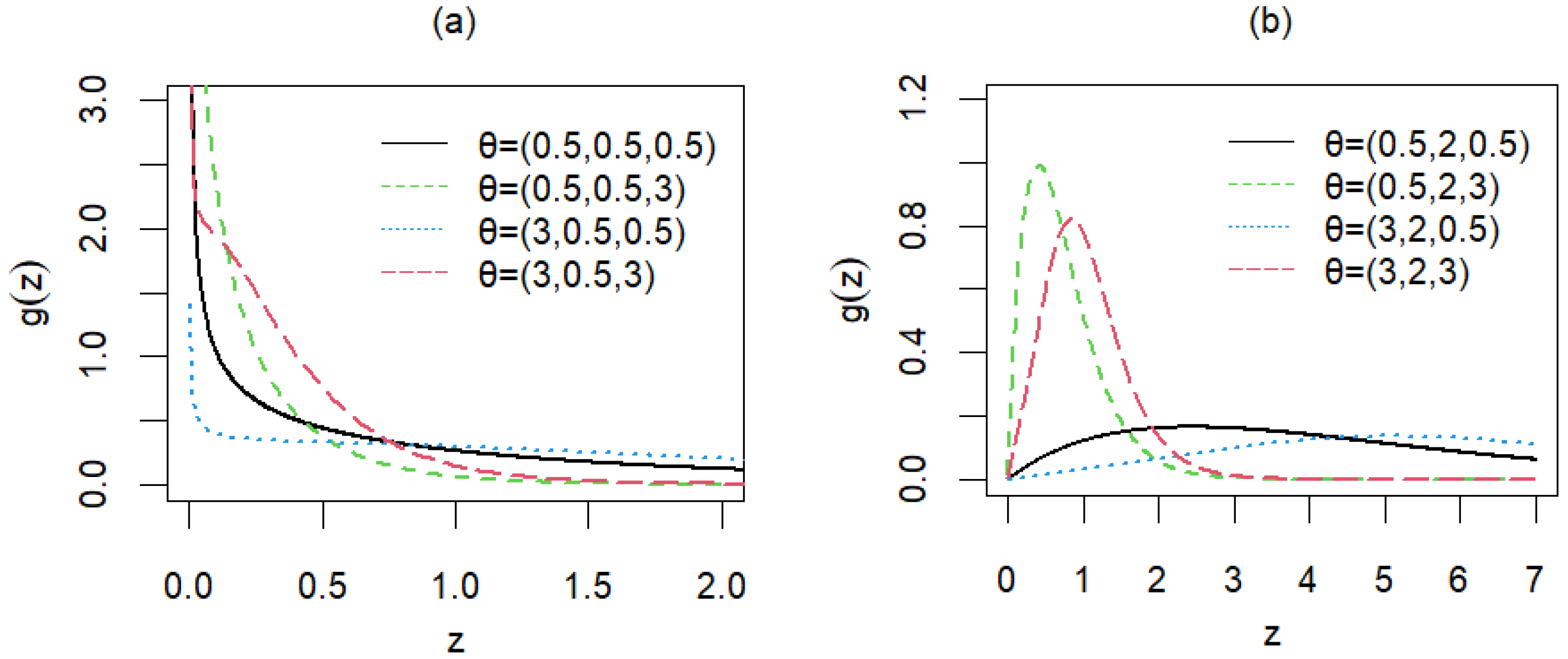
2. The Complementary Gamma Zero-Truncated Poisson Distribution

Let $X_1,X_2,\dots ,X_N$ be independent and identically distributed random variables from a gamma distribution which probability density function (pdf) given by

$$f(x;\alpha ,\beta )={\beta }^{\alpha }{x}^{\alpha -1}{e}^{-\beta x}/\mathrm{\Gamma }\left(\alpha \right),x>0,$$

where $\alpha >0$ is a shape parameter and $\beta >0$ is a rate parameter, and $N$ is a random variable from a zero-truncated Poisson distribution with parameter $\lambda >0$. The pdf is given by

$$P(N=n)=e^{-\lambda }{\lambda }^n/n!\left(1-e^{-\lambda }\right), n=1,2,\dots .$$

Assuming that random variables $X$ and $N$ are independent, we define $Z=\max \{X_1,$$X_2,\dots ,X_N\}.$ Then, $g(z|n)=n{\left[F\left(z\right)\right]}^{n-1}f(z)$, where $F\left(z\right)=1-\mathrm{\Gamma }\left(\alpha ,\beta z\right)/\mathrm{\Gamma }\left(\alpha \right),$ and $\mathrm{\Gamma }\left(\alpha ,\beta z\right)={\displaystyle \underset{\beta z}{\overset{\infty }{\int }}{t}^{\alpha -1}{e}^{-t}dt}$ is the upper incomplete gamma function. The marginal distribution for $Z$ is

$$g(z;\mathit{\theta })=\frac{\lambda e^{-\lambda }}{\left(1-e^{-\lambda }\right)}\left(\frac{{\beta }^{\alpha }{z}^{\alpha -1}{e}^{-\beta z}}{\mathrm{\Gamma }\left(\alpha \right)}\right)e^{\lambda \left(1-\frac{\mathrm{\Gamma }(\alpha ,\beta z)}{\mathrm{\Gamma }\left(\alpha \right)}\right)}, z,\lambda ,\alpha ,\beta >0,$$

(1)

where $\mathit{\theta }=\left(\lambda ,\alpha ,\beta \right)$. The distribution of $Z$ will be referred to as CGZTP, and plots of its pdf are displayed in Figure 1 for selected parameter values. For $\alpha =1$, the CGZTP distribution reduces to the density of the complementary Exponential-Poisson distribution introduced by Cancho et al. [13]. Additionally, if $\lambda \to 0$, the following theorem will show that the CGZTP distribution reduces to the two-parameter gamma distribution.

Theorem 1. 

The CGZTP distribution reduces to two-parameter gamma distribution as  $\lambda \to 0$.

Proof. 

If $\lambda$ approaches to zero, then

$$\begin{array}{cc}\hfill \underset{\lambda \to 0}{\lim }g\left(z;\mathit{\theta }\right)& =\underset{\lambda \to 0}{\lim }\frac{\lambda e^{-\lambda }}{\left(1-e^{-\lambda }\right)}\left(\frac{{\beta }^{\alpha }{z}^{\alpha -1}{e}^{-\beta z}}{\mathrm{\Gamma }\left(\alpha \right)}\right)e^{\lambda \left(1-\frac{\mathrm{\Gamma }(\alpha ,\beta z)}{\mathrm{\Gamma }\left(\alpha \right)}\right)}\hfill \\ & =\frac{{\beta }^{\alpha }{z}^{\alpha -1}{e}^{-\beta z}}{\mathrm{\Gamma }\left(\alpha \right)}.\hfill \end{array}$$

Then, the CGZTP distribution reduces to the two-parameter gamma distribution. □

3. Properties of the Distribution

3.1. Cumulative Distribution Function, Quantile and Moment

The cumulative distribution function (cdf) of the CGZTP distribution is given by:

$$G(z;\mathit{\theta })=\left(e^{-\frac{\lambda \mathrm{\Gamma }(\alpha ,\beta z)}{\mathrm{\Gamma }\left(\alpha \right)}}-e^{-\lambda }\right)/\left(1-e^{-\lambda }\right)$$

(2)

and the $r\mathrm{th}$ quantile is defined as the value $z$ such that:

$$\mathrm{\Gamma }(\alpha ,\beta z)=-\frac{\mathrm{\Gamma }\left(\alpha \right)}{\lambda }\ln \left(r+\left(1-r\right)e^{-\lambda }\right).$$

In particular, the median is $z$ such that $\mathrm{\Gamma }(\alpha ,\beta z)=-\mathrm{\Gamma }\left(\alpha \right)\ln \left(0.5+0.5e^{-\lambda }\right)/\lambda$. Additionally, the moment generating function can be calculated from:

$$M_Z(t)=\frac{\lambda {\beta }^{\alpha }}{\mathrm{\Gamma }\left(\alpha \right)\left(1-e^{-\lambda }\right)}{\displaystyle \underset{0}{\overset{\infty }{\int }}{z}^{\alpha -1}{e}^{tz-\beta z-\lambda \frac{\mathrm{\Gamma }(\alpha ,\beta z)}{\mathrm{\Gamma }\left(\alpha \right)}}dz}.$$

The $k$-th raw moments are given by:

$$E(Z^k)=\frac{\lambda {\beta }^{\alpha }}{\mathrm{\Gamma }\left(\alpha \right)\left(1-e^{-\lambda }\right)}{\displaystyle \underset{0}{\overset{\infty }{\int }}{z}^{\alpha -1+k}{e}^{-\beta z-\lambda \frac{\mathrm{\Gamma }(\alpha ,\beta z)}{\mathrm{\Gamma }\left(\alpha \right)}}dz} , k\in \mathbb{N}.$$

The raw moments have no closed form; however, the convergence of moments can be verified by employing the comparison theorem for an improper integral [14]. Suppose that:

$$m(z)=z^{\alpha -1+k}{e}^{-\beta z-\lambda \frac{\mathrm{\Gamma }(\alpha ,\beta z)}{\mathrm{\Gamma }\left(\alpha \right)}}$$

and

$$n(z)=z^{\alpha -1+k}{e}^{-\beta z}$$

are continuous functions with $0\le m(z)\le n(z)$ for $z\ge 0$. Since ${\displaystyle \underset{0}{\overset{\infty }{\int }}n(z)}dz={\beta }^{-(\alpha +k)}\mathrm{\Gamma }\left(\alpha +k\right)$, which means that this integral converges, ${\displaystyle \underset{0}{\overset{\infty }{\int }}m(z)}dz$ also converges. It follows that the raw moments of the distribution converge for all $k$. Therefore, the mean and variance of the CGZTP distribution are given, respectively, by:

$$E(Z)=\frac{\lambda {\beta }^{\alpha }}{\mathrm{\Gamma }\left(\alpha \right)\left(1-e^{-\lambda }\right)}{\displaystyle \underset{0}{\overset{\infty }{\int }}{z}^{\alpha }{e}^{-\beta z-\lambda \frac{\mathrm{\Gamma }(\alpha ,\beta z)}{\mathrm{\Gamma }\left(\alpha \right)}}dz}$$

and

$$Var(Z)=\frac{\lambda {\beta }^{\alpha }}{\mathrm{\Gamma }\left(\alpha \right)\left(1-e^{-\lambda }\right)}{\displaystyle \underset{0}{\overset{\infty }{\int }}{z}^{\alpha +1}{e}^{-\beta z-\lambda \frac{\mathrm{\Gamma }(\alpha ,\beta z)}{\mathrm{\Gamma }\left(\alpha \right)}}dz}-{\left[E(Z)\right]}^2.$$

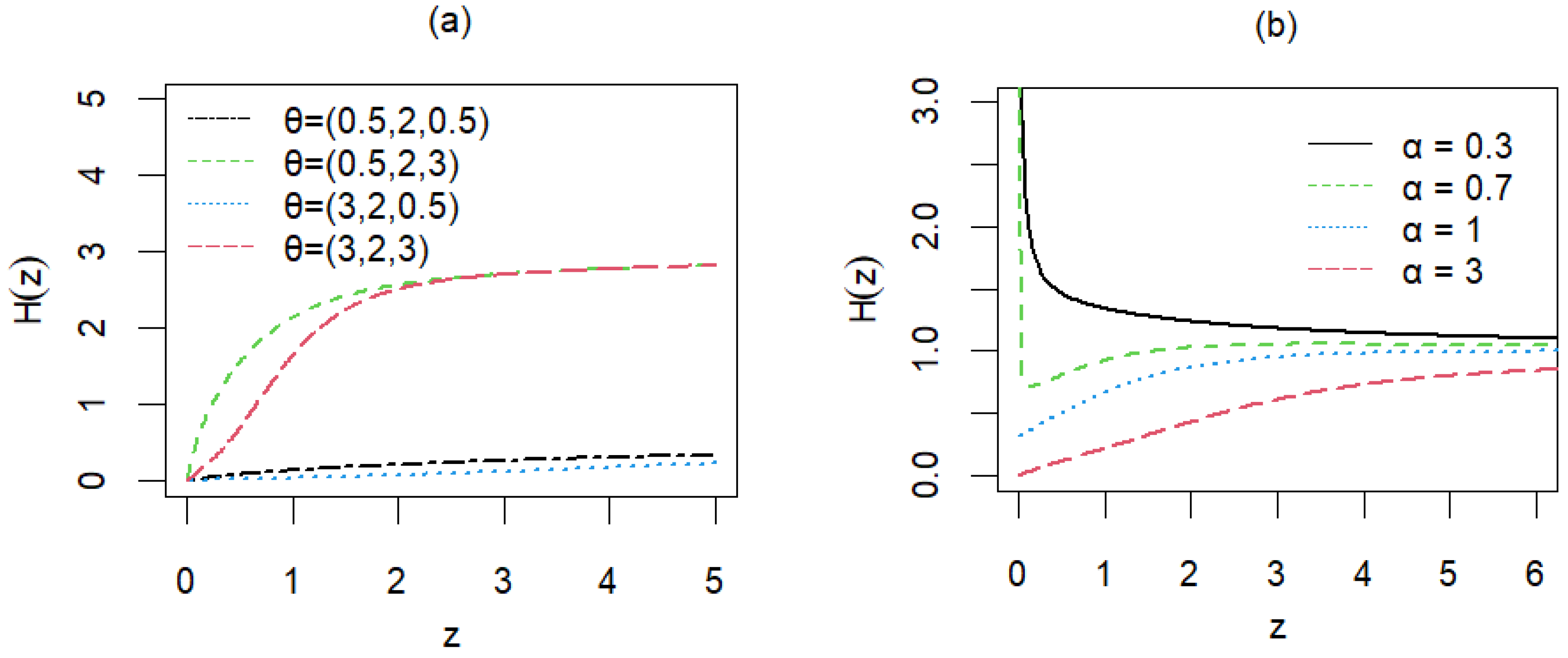
3.2. Survival Function and Hazard Function

Using Equations (1) and (2), the survival and hazard functions of the CGZTP distribution are given, respectively, by:

$$S(z;\mathit{\theta })=1-G(z;\mathit{\theta })=\frac{1-e^{-\frac{\lambda \mathrm{\Gamma }(\alpha ,\beta z)}{\mathrm{\Gamma }\left(\alpha \right)}}}{1-e^{-\lambda }}$$

and

$$H(z;\mathit{\theta })=\frac{g(z;\mathit{\theta })}{S(z;\mathit{\theta })}=\frac{\lambda {\beta }^{\alpha }{z}^{\alpha -1}{e}^{-\beta z-\frac{\lambda \mathrm{\Gamma }(\alpha ,\beta z)}{\mathrm{\Gamma }\left(\alpha \right)}}}{\mathrm{\Gamma }\left(\alpha \right)\left(1-e^{-\frac{\lambda \mathrm{\Gamma }(\alpha ,\beta z)}{\mathrm{\Gamma }\left(\alpha \right)}}\right)}.$$

If considering $\eta \left(z\right)=-\frac{g^{\prime }\left(z;\mathit{\theta }\right)}{g\left(z;\mathit{\theta }\right)}$, it is straightforward to show that:

$$\eta \left(z\right)=-\left(1/z\right)[\alpha -1-\beta z+\lambda {\left(\beta z\right)}^{\alpha }{e}^{-\beta z}/\mathrm{\Gamma }\left(\alpha \right)],$$

and its first derivative is

$${\eta }^{\prime }\left(z\right)=\frac{1}{\mathrm{\Gamma }\left(\alpha \right)z^2}\left[\left(\alpha -1\right)\mathrm{\Gamma }\left(\alpha \right)+\lambda {\left(\beta z\right)}^{\alpha }\left(\beta z-\alpha +1\right)e^{-\beta z}\right].$$

For $\alpha =1$, ${\eta }^{\prime }\left(z\right)>0$ for all $z$, the hazard function is increasing according to Glaser’s theorem [15]. However, in cases $\alpha >1$ or $0<\alpha <1$, the sign of ${\eta }^{\prime }\left(z\right)$ relates to all parameters of the distribution. For example, when $\alpha >1$, ${\eta }^{\prime }\left(z\right)$ is greater than 0 if $\beta z-\alpha +1>0$. This condition depends on the value of $z$ and parameter $\beta$. Additionally, if $\beta z-$$\alpha +1<0,$ the sign of ${\eta }^{\prime }\left(z\right)$ will follow the sign of $\left(\alpha -1\right)\mathrm{\Gamma }\left(\alpha \right)+\lambda {\left(\beta z\right)}^{\alpha }\left(\beta z-\alpha +1\right)e^{-\beta z}$. In the latter case, the shape of hazard function can be a bathtub. When $0<\alpha <1$, the sign of ${\eta }^{\prime }\left(z\right)$ will depend on the sign of $\left(\alpha -1\right)\mathrm{\Gamma }\left(\alpha \right)+\lambda {\left(\beta z\right)}^{\alpha }\left(\beta z-\alpha +1\right)e^{-\beta z}$. There are no explicit conditions that are functions of only one parameter. To check the shape of a hazard function, all related parameters are used to calculate the aforementioned conditions. Figure 2 illustrates some of the possible shapes of the hazard function for selected values of $\mathit{\theta }$. The shape of the hazard function can be increasing, decreasing or bathtub-shaped.

4. Parameter Estimation

4.1. Method of Maximum Likelihood

The log-likelihood function based on the observed random sample size of $n$, $w_{obs}=\left(z_1,z_2,\dots ,z_n\right),$ is the following:

$$\begin{array}{cc}\hfill l\left(\mathit{\theta };w_{obs}\right)& =n\left(\log \lambda -\log \left(1-e^{-\lambda }\right)\right)+n\alpha \log \beta -n\log \mathrm{\Gamma }\left(\alpha \right)+\left(\alpha -1\right){\displaystyle \sum _{i=1}^n\log z_i}\hfill \\ & -\beta \left({\displaystyle \sum _{i=1}^n{z}_i}\right)-\lambda {\displaystyle \sum _{i=1}^n\mathrm{\Gamma }\left(\alpha ,\beta z_i\right)}/\mathrm{\Gamma }\left(\alpha \right),\hfill \end{array}$$

and the corresponding gradients are found to be

$$\frac{\partial l\left(\mathit{\theta };w_{obs}\right)}{\partial \lambda }=n\left(1/\lambda -e^{-\lambda }{\left(1-e^{-\lambda }\right)}^{-1}\right)-{\displaystyle \sum _{i=1}^n\mathrm{\Gamma }\left(\alpha ,\beta z_i\right)}/\mathrm{\Gamma }\left(\alpha \right),$$

(3)

$$\frac{\partial l\left(\mathit{\theta };w_{obs}\right)}{\partial \alpha }=n\log \beta -n{\psi }_0(\alpha )+{\displaystyle \sum _{i=1}^n\log z_i}$$

$$-\lambda {\displaystyle \sum _{i=1}^n\left[G_{2,3}^{3,0}\left(\beta z_i|\begin{array}{c}1,1\\ 0,0,\alpha \end{array}\right)+\mathrm{\Gamma }(\alpha ,\beta z_i)\left(\log \left(\beta z_i\right)-{\psi }_0(\alpha )\right)\right]/\mathrm{\Gamma }\left(\alpha \right)},$$

(4)

$$\frac{\partial l\left(\mathit{\theta };w_{obs}\right)}{\partial \beta }=\frac{n\alpha }{\beta }-{\displaystyle \sum _{i=1}^n{z}_i}+\frac{\lambda {\beta }^{\alpha -1}}{\mathrm{\Gamma }\left(\alpha \right)}{\displaystyle \sum _{i=1}^n{z}_i^{\alpha }{e}^{-\beta z_i}},$$

(5)

where ${\psi }_0(\alpha )$ is a digamma function and $G_{p,q}^{m,n}\left(\beta z_i|\begin{array}{c}{a}_1,\dots a_p\\ b_1,\dots b_q\end{array}\right)$ is Meijer G-function. The Meijer G-function is a very general function which reduces to simpler special functions in many common cases [16]. It is defined by:

$$G_{p,q}^{m,n}\left(z|\begin{array}{c}{a}_1,\dots a_p\\ b_1,\dots b_q\end{array}\right)=\frac{1}{2\pi i}{\displaystyle \underset{L}{\int }\frac{{\prod }_{j=1}^m\mathrm{\Gamma }\left(b_j-s\right){\prod }_{j=1}^n\mathrm{\Gamma }\left(1-a_j+s\right)}{{\prod }_{j=m+1}^q\mathrm{\Gamma }\left(1-b_j+s\right){\prod }_{j=n+1}^p\mathrm{\Gamma }\left(a_j-s\right)}}{z}^{s}ds,$$

where the integral is a line integral along a path L in the complex plane that separates the poles of the Gamma function terms $\mathrm{\Gamma }\left(a_j-s\right)$ from the poles of the terms $\mathrm{\Gamma }\left(b_j-s\right)$. The definition of the Meijer G-function holds under the following assumptions:

(a)

$0\le m\le q$ and $0\le n\le p$ where $m,n,p$ and $q$ are integer numbers.

(b)

$a_k-b_j\ne 1,2,3,\dots$ for $k=1,2,\dots ,n$ and $j=1,2,\dots ,m$ which implies that no pole of any $\mathrm{\Gamma }\left(b_j-s\right)$,$j=1,2,\dots ,m$ coincide with any pole of any $\mathrm{\Gamma }\left(1-a_k+s\right)$,$k=1,2,\dots ,n$.

(c)

$z\ne 0$.

Here,

$$\begin{gathered} G_{2,3}^{3,0}\left(\beta z_i|\begin{array}{c}1,1\\ 0,0,\alpha \end{array}\right)=\frac{1}{2\pi i}{\displaystyle \underset{L}{\int }\frac{{\prod }_{j=1}^3\mathrm{\Gamma }\left(b_j-s\right)}{{\prod }_{j=1}^2\mathrm{\Gamma }\left(a_j-s\right)}}{\left(\beta z_i\right)}^{s}ds \\ =\frac{1}{2\pi i}{\displaystyle \underset{L}{\int }\frac{\mathrm{\Gamma }\left(-s\right)\mathrm{\Gamma }\left(-s\right)\mathrm{\Gamma }\left(\alpha -s\right)}{\mathrm{\Gamma }\left(1-s\right)\mathrm{\Gamma }\left(1-s\right)}}{\left(\beta z_i\right)}^{s}ds. \end{gathered}$$

More details on the Meijer G-function can be found in Rajshreemishra [16].

For finding the MLEs, Equation (5) could be solved exactly for $\lambda$ as follows:

$$\begin{array}{cc}\hfill \frac{\partial l\left(\mathit{\theta };w_{obs}\right)}{\partial \beta }& =0\hfill \\ \hfill \frac{n\alpha }{\beta }-{\displaystyle \sum _{i=1}^n{z}_i}+\frac{\lambda {\beta }^{\alpha -1}}{\mathrm{\Gamma }\left(\alpha \right)}{\displaystyle \sum _{i=1}^n{z}_i^{\alpha }{e}^{-\beta z_i}}& =0\hfill \\ \hfill \lambda & =\frac{\mathrm{\Gamma }\left(\alpha \right)}{{\beta }^{\alpha -1}{\displaystyle \sum _{i=1}^n{z}_i^{\alpha }{e}^{-\beta z_i}}}\left({\displaystyle \sum _{i=1}^n{z}_i}-\frac{n\alpha }{\beta }\right).\hfill \end{array}$$

Thus, the maximum likelihood estimator of $\lambda$ is $\widehat{\lambda }=\frac{\mathrm{\Gamma }\left(\widehat{\alpha }\right)}{{\widehat{\beta }}^{\widehat{\alpha }-1}{\displaystyle \sum _{i=1}^n{z}_i^{\widehat{\alpha }}{e}^{-\widehat{\beta }{z}_i}}}\left({\displaystyle \sum _{i=1}^n{z}_i}-\frac{n\widehat{\alpha }}{\widehat{\beta }}\right)$, conditional upon the value of $\widehat{\alpha }$ and $\widehat{\beta }$, where $\widehat{\lambda }$, $\widehat{\alpha }$ and $\widehat{\beta }$ are maximum likelihood estimates (MLEs) for the parameter $\lambda$, $\alpha$ and $\beta$, respectively.

In the following theorem, a condition is needed to be satisfied for the existence of the MLEs of $\lambda$ and $\beta$.

Theorem 2. 

(a)

Let $l_1\left(\lambda ;\alpha ,\beta ,w_{obs}\right)=\partial l\left(\mathit{\theta };w_{obs}\right)/\partial \lambda$, If $\alpha$ and $\beta$ are known, then$\widehat{\lambda }$ is the uniquely exist root of $l_1\left(\lambda ;\alpha ,\beta ,w_{obs}\right)=0$ if ${\displaystyle \sum _{i=1}^n\mathrm{\Gamma }\left(\alpha ,\beta z_i\right)}/\mathrm{\Gamma }\left(\alpha \right)<\frac{n}{2}$.

Proof. 

Since $l_1\left(\lambda ;\alpha ,\beta ,w_{obs}\right)=n\left(\frac{1}{\lambda }-\frac{e^{-\lambda }}{1-e^{-\lambda }}\right)-{\displaystyle \sum _{i=1}^n\mathrm{\Gamma }\left(\alpha ,\beta z_i\right)}/\mathrm{\Gamma }\left(\alpha \right)$,

$$\underset{\lambda \to 0}{\lim }{l}_1\left(\lambda ;\alpha ,\beta ,w_{obs}\right)=\frac{n}{2}-{\displaystyle \sum _{i=1}^n\mathrm{\Gamma }\left(\alpha ,\beta z_i\right)}/\mathrm{\Gamma }\left(\alpha \right)$$

and

$$\underset{\lambda \to \infty }{\lim }{l}_1\left(\lambda ;\alpha ,\beta ,w_{obs}\right)=-{\displaystyle \sum _{i=1}^n\mathrm{\Gamma }\left(\alpha ,\beta z_i\right)}/\mathrm{\Gamma }\left(\alpha \right).$$

Because $\underset{\lambda \to 0}{\lim }{l}_1\left(\lambda ;\alpha ,\beta ,w_{obs}\right)>0$ as ${\displaystyle \sum _{i=1}^n\mathrm{\Gamma }\left(\alpha ,\beta z_i\right)}/\mathrm{\Gamma }\left(\alpha \right)<\frac{n}{2}$ and $\underset{\lambda \to \infty }{\lim }{l}_1\left(\lambda ;\alpha ,\beta ,w_{obs}\right)<0$, there exists at least one solution of $l_1\left(\lambda ;\alpha ,\beta ,w_{obs}\right)=0$. Consider

$$l_1{}^{\prime }\left(\lambda ;\alpha ,\beta ,w_{obs}\right)=-\frac{n{e}^{\lambda }(e^{-\lambda }+e^{\lambda }-({\lambda }^2+2))}{e^{\lambda }}$$

and use the fact that $e^{\lambda }=1+\lambda +\frac{1}{2}{\lambda }^2+\frac{1}{3!}{\lambda }^3+\dots$ and $e^{-\lambda }=1-\lambda +\frac{1}{2}{\lambda }^2-\frac{1}{3!}{\lambda }^3+\dots$, then $e^{-\lambda }+e^{\lambda }=2+{\lambda }^2+\frac{2}{4!}{\lambda }^4+\dots >{\lambda }^2+2$. It follows that $l_1{}^{\prime }\left(\lambda ;\alpha ,\beta ,w_{obs}\right)<0$ and $l_1$ is strictly decreasing in $\lambda$. Consequently, the root is proved to be unique. □

(b)

Let $l_3\left(\beta ;\lambda ,\alpha ,w_{obs}\right)=\partial l\left(\mathit{\theta };w_{obs}\right)/\partial \beta$. If $\lambda$ and $\alpha$ are known, then there exists at least one solution of $l_3\left(\beta ;\lambda ,\alpha ,w_{obs}\right)=0$.

Proof. 

Because $l_3\left(\beta ;\lambda ,\alpha ,w_{obs}\right)=\frac{n\alpha }{\beta }-{\displaystyle \sum _{i=1}^n{z}_i}+\frac{\lambda {\beta }^{\alpha -1}}{\mathrm{\Gamma }\left(\alpha \right)}{\displaystyle \sum _{i=1}^n{z}_i^{\alpha }{e}^{-\beta z_i}}$,

$$\underset{\beta \to 0}{\lim }{l}_3\left(\beta ;\lambda ,\alpha ,w_{obs}\right)=\underset{\beta \to 0}{\lim }\frac{n\alpha }{\beta }-\underset{\beta \to 0}{\lim }{\displaystyle \sum _{i=1}^n{z}_i}+\underset{\beta \to 0}{\lim }\frac{\lambda {\beta }^{\alpha -1}}{\mathrm{\Gamma }\left(\alpha \right)}{\displaystyle \sum _{i=1}^n{z}_i^{\alpha }{e}^{-\beta z_i}}=\infty$$

and

$$\begin{array}{cc}\hfill \underset{\beta \to \infty }{\lim }{l}_3\left(\beta ;\lambda ,\alpha ,w_{obs}\right)& =\underset{\beta \to \infty }{\lim }\frac{n\alpha }{\beta }-\underset{\beta \to \infty }{\lim }{\displaystyle \sum _{i=1}^n{z}_i}+\underset{\beta \to \infty }{\lim }\frac{\lambda {\beta }^{\alpha -1}}{\mathrm{\Gamma }\left(\alpha \right)}{\displaystyle \sum _{i=1}^n{z}_i^{\alpha }{e}^{-\beta z_i}}\hfill \\ & =0-{\displaystyle \sum _{i=1}^n{z}_i}+\underset{\beta \to \infty }{\lim }\frac{\lambda {\beta }^{\alpha -1}}{\mathrm{\Gamma }\left(\alpha \right)}{\displaystyle \sum _{i=1}^n{z}_i^{\alpha }{e}^{-\beta z_i}}\hfill \\ & =-{\displaystyle \sum _{i=1}^n{z}_i}+\underset{\beta \to \infty }{\lim }\frac{\lambda {\beta }^{\alpha -1}}{\mathrm{\Gamma }\left(\alpha \right)}{\displaystyle \sum _{i=1}^n{z}_i^{\alpha }{e}^{-\beta z_i}}.\hfill \end{array}$$

Consider the following:

$$\underset{\beta \to \infty }{\lim }\frac{\lambda {\beta }^{\alpha -1}}{\mathrm{\Gamma }\left(\alpha \right)}{\displaystyle \sum _{i=1}^n{z}_i^{\alpha }{e}^{-\beta z_i}}=\frac{\lambda }{\mathrm{\Gamma }\left(\alpha \right)}{\displaystyle \sum _{i=1}^n\left(z_i\underset{\beta \to \infty }{\lim }\frac{{\left(\beta z_i\right)}^{\alpha -1}}{e^{\beta z_i}}\right)}.$$

Since $\underset{\beta \to \infty }{\lim }\frac{{\left(\beta z_i\right)}^{\alpha -1}}{e^{\beta z_i}}=0$, $\underset{\beta \to \infty }{\lim }\frac{\lambda {\beta }^{\alpha -1}}{\mathrm{\Gamma }\left(\alpha \right)}{\displaystyle \sum _{i=1}^n{z}_i^{\alpha }{e}^{-\beta z_i}}=0$. It leads to $\underset{\beta \to \infty }{\lim }{l}_3\left(\beta ;\lambda ,\alpha ,w_{obs}\right)=-{\displaystyle \sum _{i=1}^n{z}_i}<0.$

Therefore, there exist at least one solution of $l_3\left(\beta ;\lambda ,\alpha ,w_{obs}\right)=0$. □

4.2. Variance–Covariance Matrix of the MLEs

The MLE of $\mathit{\theta }$ is approximately multivariate normal with a mean $\mathit{\theta }$ and a variance–covariance matrix that is the inverse of Fisher information matrix, i.e., $\hat{\mathit{\theta }}\sim N_3\left(\mathit{\theta },J{\left(\hat{\mathit{\theta }}\right)}^{-1}\right)$ or $\hat{\mathit{\theta }}\sim N_3\left(\mathit{\theta },I{\left(\hat{\mathit{\theta }}\right)}^{-1}\right),$ where $J\left(\mathit{\theta }\right)=E\left[I\left(\mathit{\theta }\right)\right]$ and $I\left(\mathit{\theta }\right)$ is the observed Fisher information matrix. By differentiating Equations (3)–(5), the elements of the observed Fisher information matrix are derived as follows:

$$I_{11}=n{e}^{\lambda }(e^{-\lambda }+e^{\lambda }-({\lambda }^2+2))/e^{\lambda },$$

$$I_{22}=n{\psi }^{(1)}(\alpha )+\lambda {\displaystyle \sum _{i=1}^n\left[\frac{1}{\mathrm{\Gamma }\left(\alpha \right)}\left(\begin{array}{l}2G_{3,4}^{4,0}\left(\beta z_i|\begin{array}{c}1,1,1\\ 0,0,0,\alpha \end{array}\right)+2\left(\log \left(\beta z_i\right)-{\psi }^{(0)}\left(\alpha \right)\right)G_{2,3}^{3,0}\left(\beta z_i|\begin{array}{c}1,1\\ 0,0,\alpha \end{array}\right)\\ +\mathrm{\Gamma }\left(\alpha ,\beta z_i\right)\left(-2{\psi }^{\left(0\right)}\left(\alpha \right)\log (\beta z_i)+{\psi }^{\left(0\right)}{\left(\alpha \right)}^2-{\psi }^{\left(1\right)}\left(\alpha \right)+{\log }^2(\beta z_i)\right)\end{array}\right)\right]},$$

$$I_{33}=\frac{n\alpha }{{\beta }^2}-\frac{\lambda {\beta }^{\alpha -2}}{\mathrm{\Gamma }\left(\alpha \right)}{\displaystyle \sum _{i=1}^n{z}_i^{\alpha }{e}^{-\beta z_i}\left(\alpha -1-\beta z_i\right)},$$

$$I_{12}=I_{21}=\left(1/\mathrm{\Gamma }\left(\alpha \right)\right){\displaystyle \sum _{i=1}^n{G}_{2,3}^{3,0}\left(\beta z_i|\begin{array}{c}1,1\\ 0,0,\alpha \end{array}\right)+\mathrm{\Gamma }(\alpha ,\beta z_i)\left(\log \left(\beta z_i\right)-{\psi }_0(\alpha )\right)},$$

$$I_{13}=I_{31}=-\lambda {\beta }^{\alpha -1}\left(1/\mathrm{\Gamma }\left(\alpha \right)\right){\displaystyle \sum _{i=1}^n{z}_i^{\alpha }{e}^{-\beta z_i}},$$

$$\begin{array}{l}{I}_{23}=I_{32}=-\frac{n}{\beta }-\lambda {\displaystyle \sum _{i=1}^n{e}^{-\beta z_i}\frac{\partial }{\partial \alpha }\left[\frac{z_i^{\alpha }{\beta }^{\alpha -1}}{\mathrm{\Gamma }\left(\alpha \right)}\right]}=-\frac{n}{\beta }-\lambda {\displaystyle \sum _{i=1}^n{e}^{-\beta z_i}\left[\frac{z_i^{\alpha }{\beta }^{\alpha -1}\left(-{\psi }^{(0)}(\alpha )+\log (\beta )+\log (z_i)\right)}{\mathrm{\Gamma }\left(\alpha \right)}\right]}.\\ \end{array}$$

4.3. Asymptotic Confidence Interval

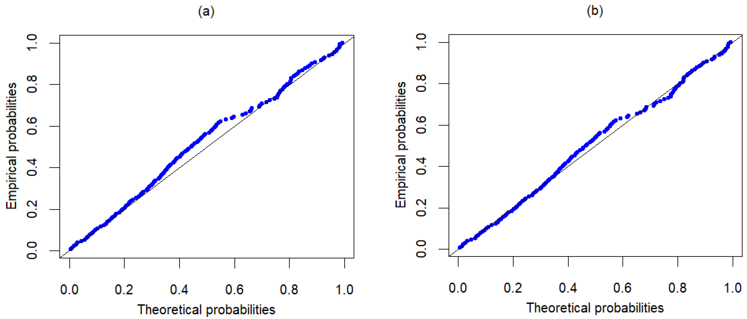
The Wald Confidence Interval is a type of confidence interval based on asymptotic theory or large-sample theory. This means that the interval’s coverage probability approaches the nominal level as the sample size goes to infinity. For testing the null hypothesis $H_0:\mathit{\theta }={\mathit{\theta }}_0$, the test statistic is the Wald statistic:

$$J{\left(\hat{\mathit{\theta }}\right)}^{1/2}\left(\hat{\mathit{\theta }}-{\mathit{\theta }}_0\right)\sim N_3\left(0,I_3\right) \mathrm{or} I{\left(\hat{\mathit{\theta }}\right)}^{1/2}\left(\hat{\mathit{\theta }}-{\mathit{\theta }}_0\right)\sim N_3\left(0,I_3\right).$$

The asymptotic distribution of the ith component of $\hat{\mathit{\theta }}$ is ${\widehat{\theta }}_i\sim N\left({\theta }_i,J^{ii}\right)$ or ${\widehat{\theta }}_i\sim N\left({\theta }_i,I^{ii}\right)$, where $J^{ii}={\left[J{\left(\widehat{\theta }\right)}^{-1}\right]}_{ii}$ and $I^{ii}={\left[I{\left(\widehat{\theta }\right)}^{-1}\right]}_{ii}$. Then, the corresponding $\left(1-\alpha \right)100\%$ Wald confidence intervals for ${\theta }_i$ are ${\widehat{\theta }}_i\pm z_{1-\alpha /2}\sqrt{J^{ii}}$ or ${\widehat{\theta }}_i\pm z_{1-\alpha /2}\sqrt{I^{ii}}$.

5. Simulation Study

The samples were generated by using the rejection sampling method. The study was based on 1000 simulated samples from the CGZTPs with different sample sizes: n = 50, 100 and 1000. The case studies are CGZTP $\left(\lambda =1,\alpha =2,\beta =1\right)$, CGZTP $\left(\lambda =3,\alpha =1,\beta =0.5\right)$ and CGZTP $\left(\lambda =3,\alpha =0.5,\beta =0.5\right)$. When all parameters are assumed unknown, the MLEs of $\lambda , \alpha$ and $\beta$ are numerically calculated by the simulated-annealing method. In the simulated annealing optimization algorithm, each potential solution to an optimization problem is viewed as a state of a physical system, and each state has an associated energy calculated from the objective function of the optimization problem. The system attempts to move to a state of lower energy to reduce the overall system’s energy. The R package “maxLik” version 1.5-2 was used to find the MLEs as well as the hessian of log-likelihood functions.

Table 1. Mean estimates, minimum and maximum values of estimated parameters and mean-squared errors of $\lambda , \alpha ,$ and $\beta$.

Distribution	n	Estimator	Mean Estimate	Min	Max	MSE
CGZTP (1,2,1)	50	$\widehat{\lambda }$	1.7122	0.0001	17.6696	5.3198
		$\widehat{\alpha }$	1.9225	0.1245	4.3819	0.4782
		$\widehat{\beta }$	1.0064	0.4106	1.9742	0.0519
	100	$\widehat{\lambda }$	1.6464	0.0002	15.5108	4.5325
		$\widehat{\alpha }$	1.8901	0.2544	3.9272	0.3659
		$\widehat{\beta }$	0.9864	0.5593	1.6377	0.0272
	1000	$\widehat{\lambda }$	1.0225	0.0005	7.3604	0.3992
		$\widehat{\alpha }$	2.0003	0.5176	2.5456	0.0523
		$\widehat{\beta }$	0.9965	0.6622	1.1687	0.0025
CGZTP (3,1,0.5)	50	$\widehat{\lambda }$	2.2571	0.0020	12.5656	4.4487
		$\widehat{\alpha }$	1.4061	0.1748	3.1618	0.5402
		$\widehat{\beta }$	0.5503	0.2714	1.1914	0.0193
	100	$\widehat{\lambda }$	2.4622	0.0027	10.0311	3.4684
		$\widehat{\alpha }$	1.2759	0.2918	2.7858	0.3293
		$\widehat{\beta }$	0.5294	0.3194	0.8996	0.0092
	1000	$\widehat{\lambda }$	2.9382	0.7820	7.2618	0.8841
		$\widehat{\alpha }$	1.0504	0.3924	1.7449	0.0597
		$\widehat{\beta }$	0.5049	0.3728	0.6275	0.0015
CGZTP (3,0.5,0.5)	50	$\widehat{\lambda }$	2.3268	0.0015	14.3020	4.5848
		$\widehat{\alpha }$	0.715	0.0946	1.8241	0.1518
		$\widehat{\beta }$	0.5386	0.2916	1.0680	0.0165
	100	$\widehat{\lambda }$	2.5139	0.0002	12.7619	3.679
		$\widehat{\alpha }$	0.6553	0.0989	1.4855	0.0981
		$\widehat{\beta }$	0.5265	0.3043	0.8963	0.0086
	1000	$\widehat{\lambda }$	2.853	0.5444	7.7735	0.7855
		$\widehat{\alpha }$	0.5561	0.1756	0.9525	0.0159
		$\widehat{\beta }$	0.5098	0.3992	0.6041	0.0010

shows the average MLEs of $\lambda , \alpha$ and $\beta$, the minimum and maximum values of each estimated parameter, and their corresponding mean-squared errors (MSEs). As sample sizes increase, estimates become more accurate, and MSE values decrease. Among three estimates, $\widehat{\beta }$ tends to have smallest MSE. Additionally, the minimum and maximum values illustrate that as the sample size increases, those values of $\widehat{\alpha }$ and $\widehat{\beta }$ will get closer to the parameter values.

Wald confidence intervals using observed Fisher information are constructed for all parameters of CGZTPs. Monte Carlo simulations with 1000 repetitions help estimate the coverage probability (CP) and average length (AL) of the confidence intervals (CIs). All results are presented in

Table 2. Coverage probabilities and average lengths of Wald CIs.

$\mathit{\theta }=\left(\mathit{\lambda },\mathit{\alpha },\mathit{\beta }\right)$		$\mathit{n}$	CP	AL
$\lambda =0.5,\beta =3$	$\alpha =1$	50	0.9130	1.4147
		100	0.9090	1.0495
		1000	0.9530	0.3411
	$\alpha =2$	50	0.8920	2.6400
		100	0.9130	1.9795
		1000	0.9550	0.6626
$\alpha =1,\beta =3$	$\lambda =0.5$	50	0.9800	6.0251
		100	0.9610	4.5462
		1000	0.9520	1.3820
	$\lambda =1$	50	0.9840	6.2418
		100	0.9580	5.2028
		1000	0.9560	1.7814
$\lambda =1,\alpha =0.5$	$\beta =0.5$	50	0.9670	0.5587
		100	0.9640	0.3832
		1000	0.9470	0.1144
	$\beta =1$	50	0.9710	1.0991
		100	0.9630	0.7861
		1000	0.9530	0.2311

. It is found that when the sample size ($n$) increases, the CPs will be closer to the nominal coverage probability, 0.95, and the ALs will decrease. In a few cases, especially when $\lambda$ has a small value, i.e., $\lambda =0.5$, $n$ is required to be 1000 to achieve the nominal coverage probability. In many cases, CPs are not less than 0.95 although the sample size is only 50.

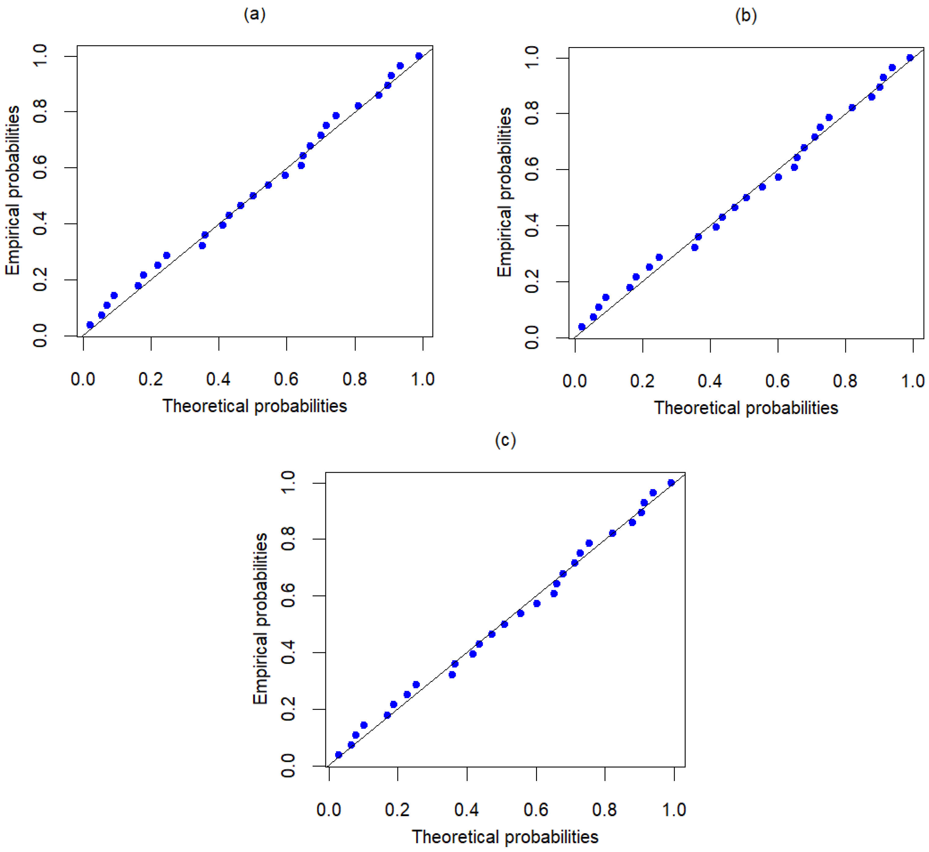
6. Application on Real Data

In this section, three real datasets are used to illustrate the use of the proposed CGZTP distribution. It is worth noting that the simulated-annealing method is used for the numerical computation of MLEs, and the model comparison is conducted using the Kolmogorov–Smirnov (K-S) test and Akaike’s information criterion (AIC).

6.1. The Number of Successive Failures

The dataset is obtained from Proschan [17], and it is made up of 213 observations about how many times the air conditioning system on each of 13 Boeing 720 jet planes failed in a row. Some descriptive statistics are presented in

Table 3. Descriptive statistics of the number of successive failures.

$\mathit{n}$	Minimum	Maximum	Median	Mean	Skewness	SD
213	1.00	603.00	57.00	93.14	1.6665	106.7636

. The gamma distribution, for which the probability density function is shown below, was also fitted to the dataset.

$$f_1(z;{\mathit{\theta }}_1)=\frac{{\beta }^{\alpha }{z}^{\alpha -1}{e}^{-\beta z}}{\mathrm{\Gamma }\left(\alpha \right)}, \mathrm{z}>0 , {\mathit{\theta }}_1=\left(\alpha ,\beta \right).$$

The p-values of the K-S tests shown in

Table 4. Maximum likelihood estimates, goodness-of-fit testing and AIC for the number of successive failure dataset.

Distribution	Estimates	K-S	p-Value	AIC
CGZTP	$\hat{\mathit{\theta }}=\left(0.1096, 0.8411, 0.0096\right)$	0.0561	0.5136	2364.206
Gamma	${\hat{\mathit{\theta }}}_1=\left(0.9048, 0.0098\right)$	0.0574	0.4826	2360.642

suggest that both CGZTP and gamma distributions are useful for fitting the dataset. When comparing p-values, CGZTP will be a better fit for the dataset as the larger p-value is under the CGZTP distribution. Nevertheless, the AIC suggests the choice of the gamma distribution. The probability–probability plots (P-P plots), given in Figure 3, show that most points under CGZTP lie not far from a straight diagonal line from the bottom left to the top right of the plot. Therefore, the CGZTP distribution can be used to model data for which the MLE of $\lambda , \alpha$ and $\beta$ are 0.11, 0.84 and 0.01, respectively.

6.2. March Precipitation

This dataset is obtained from Hinkley [18], and it is made up of 30 consecutive measurements of the amount of precipitation that fell in March in Minneapolis/St. Paul. The lists of some descriptive statistics are shown in

Table 5. Descriptive statistics of March precipitation.

$\mathit{n}$	Minimum	Maximum	Median	Mean	Skewness	SD
30	0.320	4.750	1.470	1.675	1.1447	1.0006

. Because the data have a unimodal density function and an increasing hazard function, the CGZTP, gamma and WP distributions are used to model the data. The pdf of WP is given below:

$$\mathrm{WP}: f_2\left(z;{\mathit{\theta }}_2\right)=\frac{\alpha \beta \lambda z^{\alpha -1}}{1-e^{-\lambda }}{e}^{-\lambda -\beta z^{\alpha }+\lambda e^{-\beta z^{\alpha }}}, \mathrm{z}>0 , {\mathit{\theta }}_2=\left(\lambda ,\alpha ,\beta \right).$$

The MLEs and statistics for model selections are summarized in

Table 6. Maximum likelihood estimates, goodness-of-fit testing and AIC for March precipitation dataset.

Distribution	Estimates	K-S	p-Value	AIC
CGZTP	$\hat{\mathit{\theta }}=\left(0.3811, 3.1587, 1.7838\right)$	0.05480	0.9999906	82.221
Gamma	${\hat{\mathit{\theta }}}_1=\left(2.9677, 1.7718\right)$	0.05552	0.9999868	80.197
WP	${\hat{\mathit{\theta }}}_2=\left(2.1745, 2.1041, 0.1358\right)$	0.05709	0.9999734	82.506

and suggest that all distributions can be used to model the data at a significant level of 0.05. The K–S test statistic has the smallest value and the largest p-value under the CGZTP distribution, while the AIC of the gamma fit is the lowest. Here, the “best” model depends on the choice of criteria; however, all these distributions are still useful, and the P–P plots, given in Figure 4, confirm the fit of the CGZTP, Gamma, and WP distributions to the dataset.

6.3. Breaking Stress of Carbon Fibers

The data, which were provided by Nichols and Padgett [19], consist of 100 observations of the breaking stress of 50 mm-long carbon fibers. The lists of some descriptive statistics are shown in

Table 7. Descriptive statistics of breaking stress of carbon fibers.

$\mathit{n}$	Minimum	Maximum	Median	Mean	Skewness	SD
100	0.390	5.560	2.700	2.621	0.3738	1.0139

. The gamma and CGZTP were utilized to model the breaking stress dataset, and the maximum likelihood estimates, K-S statistics and AIC are summarized in

Table 8. Maximum likelihood estimates, goodness-of-fit testing and AIC for breaking stress of carbon fibers dataset.

Distribution	Estimates	K-S	p-Value	AIC
CGZTP	$\hat{\mathit{\theta }}=\left(2.2899, 4.4108, 2.1769\right)$	0.0788	0.5639	289.334
Gamma	${\hat{\mathit{\theta }}}_1=\left(5.9511, 2.2699\right)$	0.0933	0.3484	290.467

. Under CGZTP, the p-value is larger, and the AIC value is smaller compared to the gamma distribution. This implies that the CGZTP distribution is superior to the gamma distribution according to two criteria. From Figure 5, comparing CGZTP and gamma distributions, most points under CGZTP are closer to the straight line, which confirms the fit of CGZTP to the dataset.

7. Conclusions

The gamma and zero-truncated Poisson distributions are compounded to create the CGZTP distribution. Its basic statistical properties are established in this work. The plots of hazard functions show the flexibility of this distribution, as they can be increasing, decreasing or bathtub-shaped. The MLEs and the corresponding variance–covariance matrix are mathematically derived, and some proofs of their existence and uniqueness are provided. Furthermore, a simulation study was also conducted to show the ability of parameter estimation and the quality of estimation in some case studies. The Wald confidence intervals are useful, although the samples are not large. In a few cases, large sample sizes are required to achieve the nominal level. Finally, the CGZTP model was applied to real data to demonstrate the distribution’s utility.

References

1. Adamidis, K.; Loukas, S. A Lifetime Distribution with Decreasing Failure Rate. Stat. Probab. Lett. 1998, 39, 35–42. [Google Scholar] [CrossRef]
2. Louzada, F.; Roman, M.; Cancho, V.G. The Complementary Exponential Geometric Distribution: Model, Properties, and a Comparison with Its Counterpart. Comput. Stat. Data Anal. 2011, 55, 2516–2524. [Google Scholar] [CrossRef]
3. Barreto-Souza, W.; de Morais, A.L.; Cordeiro, G.M. The Weibull-Geometric Distribution. J. Stat. Comput. Simul. 2011, 81, 645–657. [Google Scholar] [CrossRef] [Green Version]
4. Tojeiro, C.; Louzada, F.; Roman, M.; Borges, P. The Complementary Weibull Geometric Distribution. J. Stat. Comput. Simul. 2014, 84, 1345–1362. [Google Scholar] [CrossRef]
5. Zakerzadeh, H.; Mahmoudi, E. A New Two Parameter Lifetime Distribution: Model and Properties. arXiv 2012, arXiv:1204.4248. [Google Scholar]
6. Gui, W.; Zhang, H.; Guo, L. The Complementary Lindley-Geometric Distribution and Its Application in Lifetime Analysis. Sankhya B 2017, 79, 316–335. [Google Scholar] [CrossRef]
7. Kuş, C. A New Lifetime Distribution. Comput. Stat. Data Anal. 2007, 51, 4497–4509. [Google Scholar] [CrossRef]
8. Hemmati, F.; Khorram, E.; Rezakhah, S. A New Three-Parameter Ageing Distribution. J. Stat. Plan. Inference 2011, 141, 2266–2275. [Google Scholar] [CrossRef]
9. Lu, W.; Shi, D. A New Compounding Life Distribution: The Weibull–Poisson Distribution. J. Appl. Stat. 2012, 39, 21–38. [Google Scholar] [CrossRef]
10. Ismail, E. The Complementary Compound Truncated Poisson-Weibull Distribution for Pricing Catastrophic Bonds for Extreme Earthquakes. Br. J. Econ. Manag. Trade 2016, 14, 1–9. [Google Scholar] [CrossRef] [PubMed]
11. Alkarni, S.; Oraby, A. A Compound Class of Poisson and Lifetime Distributions. J. Stat. Appl. Probab. 2012, 1, 45–51. [Google Scholar] [CrossRef]
12. Gui, W.; Zhang, S.; Lu, X. The Lindley-Poisson Distribution in Lifetime Analysis and Its Properties. Hacet. J. Math. Stat. 2014, 43, 1063–1077. [Google Scholar] [CrossRef]
13. Cancho, V.G.; Louzada-Neto, F.; Barriga, G.D.C. The Poisson-Exponential Lifetime Distribution. Comput. Stat. Data Anal. 2011, 55, 677–686. [Google Scholar] [CrossRef]
14. Stewart, J. Calculus, 8th ed.; Cengage Learning: Florence, Italy, 2015; pp. 567–576. [Google Scholar]
15. Glaser, R.E. Bathtub and Related Failure Rate Characterizations. J. Am. Stat. Assoc. 1980, 75, 667–672. [Google Scholar] [CrossRef]
16. Rajshreemishra, K.R. Research scholar in the department of SOMAAS, Jiwaji University Gwalior. A Note on Natural Transformation & Meijer’s G-Function. Int. J. Math. Comput. Res. 2022, 10, 2630–2632. [Google Scholar] [CrossRef]
17. Proschan, F. Theoretical Explanation of Observed Decreasing Failure Rate. Technometrics 1963, 5, 375–383. [Google Scholar] [CrossRef]
18. Hinkley, D. On Quick Choice of Power Transformation. J. R. Stat. Soc. Ser. C. Appl. Stat. 1977, 26, 67–69. [Google Scholar] [CrossRef]
19. Nichols, M.D.; Padgett, W.J. A Bootstrap Control Chart for Weibull Percentiles. Qual. Reliab. Eng. Int. 2006, 22, 141–151. [Google Scholar] [CrossRef]
Figure 1. Probability density functions of the CGZTP distribution for (a α = 0.5  and (b α = 2 .
Mathematics 11 02584 g001
Figure 2. Hazard functions of the CGZTP distribution for (a α = 2  and (b λ = 2 ,   β = 1 .
Mathematics 11 02584 g002
Figure 3. P-P plots for the number of successive failures for (a) CGZTP and (b) Gamma distributions.
Mathematics 11 02584 g003
Figure 4. P-P plots for the March precipitation for (a) CGZTP, (b) Gamma and (c) WP distributions.
Mathematics 11 02584 g004
Figure 5. P-P plots for breaking stress of carbon fibers for (a) CGZTP and (b) Gamma distributions.
Mathematics 11 02584 g005