An Efficient Metaheuristic Algorithm for Job Shop Scheduling in a Dynamic Environment

Abstract

This paper proposes an Improved Multi-phase Particle Swarm Optimization (IMPPSO) to solve a Dynamic Job Shop Scheduling Problem (DJSSP) known as an non-deterministic polynomial-time hard (NP-hard) problem. A cellular neighbor network, a velocity reinitialization strategy, a randomly select sub-dimension strategy, and a constraint handling function are introduced in the IMPPSO. The IMPPSO is used to solve the Kundakcı and Kulak problem set and is compared with the original Multi-phase Particle Swarm Optimization (MPPSO) and Heuristic Kalman Algorithm (HKA). The results show that the IMPPSO has better global exploration capability and convergence. The IMPPSO has improved fitness for most of the benchmark instances of the Kundakcı and Kulak problem set, with an average improvement rate of 5.16% compared to the Genetic Algorithm-Mixed (GAM) and of 0.74% compared to HKA. The performance of the IMPPSO for solving real-world problems is verified by a case study. The high level of operational efficiency is also evaluated and demonstrated by proposing a simulation model capable of using the decision-making algorithm in a real-world environment.

1. Introduction

In a world where dynamic events are becoming more frequent and their impact on the production system is becoming more complex, effective production planning and scheduling are the key to achieving a company’s global competitiveness. The proper timing of dynamic events in real time can be a major challenge on a day-to-day basis. The importance of proper scheduling has been recognized in research for many decades [1].

The research trend is increasingly directed toward the proper dynamic optimization of production systems [2]. Comparative studies by researchers [3] have shown why artificial intelligence methods [4] are among the most appropriate for solving dynamic events (machine breakdown, changes in processing times, arrival of new orders, etc.) [5]. The researchers’ results [6] state that using only one artificial intelligence method does not address the complexity of the multi-objective optimization of the Dynamic Job Shop Scheduling Problem (DJSSP) optimization problem [7]. Therefore, the researchers’ results show that the development of different hybrid methods is reasonable. In hybridization, researchers combine the advantages of each method and remove their limitations, improving their performance and robustness [8,9]. In reality, the complexity of the DJSSP problem is reflected in the flexibility of the production system where the correct mathematical formulation allows the algorithm to respond quickly and efficiently [10]. The fast adaptation of the proposed algorithms [11] enables effective solutions with the reliable automatic processing of dynamic events and changes in the system [12,13]. Despite the shortcomings of certain methods, such as priority rules, their proliferation in commercial use proves useful in today’s world [14]. In the age of Industry 4.0 and the ability to create digital twins that are justified in terms of time and costs [15], the use of an effective supporting simulation model is critical in any case. The potential of a data-driven simulation model [16] that captures large amounts of data in real time [17] provides a link between an effective decision algorithm and a real-world production or service process. The era of Industry 4.0 highlights the importance of optimized dynamic production systems [18] where commercial tools are no longer the only way to achieve satisfactory operation; the need for self-developed solutions is the key to achieving global competitiveness [19]. The optimization of key production parameters [20,21] goes far beyond the scope of simple simulation interfaces [22] and expresses the need for highly connectable and powerful supporting simulation environments [23].

The limitations of the presented work refer to the lack of an efficient methodology for solving dynamic events and, in most cases, to the lack of transfer of the decision-making methods to real-world applications [24]. The main motivation of the presented research work is to demonstrate the importance of developing an effective decision-making algorithm to solve the DJSSP optimization problem. The objective is to demonstrate the effectiveness of the proposed algorithm using test data sets (to allow efficient comparison of the decision-making results of the proposed algorithm with the existing solutions) and to test it using data sets from a real-world production system supported by a simulation modelling method. The main contribution of the research work is related to the evaluation of the effectiveness of the newly proposed algorithm and shows the importance of using simulation environments in which the decision-making logic and solution scheme of the proposed algorithm can be integrated. Through the compatibility and adaptability of the system, we aim to enable a comprehensive optimization system that facilitates the user’s daily production planning in dynamic events with the main objective of achieving the company’s competitiveness in terms of cost and time in the global market.

2. Problem Description

A DJSSP is a combinatorial optimization problem where we have $n$ jobs specified in the introduction and $n^{\prime }$ jobs arrive after the scheduled start of $n$ jobs. All job orders ($n$ and $n^{\prime }$) must be executed on $m$ available machines. When considering DJSSP further, the constraints are as follows [25]:

• All machines from a set of $m$ are available at time 0;
• A single operation can only be executed on one machine at a time;
• A single machine $i$ can only execute one operation at a time;
• The operation executed on machine $i$ can only be interrupted if a dynamic event occurs (machine breakdown, new job arrival or process time change);
• The next operation cannot be executed until the previous operation is completed;
• The processing times of the operation and the assigned machine $i$ are known in advance. During a single operation, the processing time may change due to a dynamic event that changes the original processing time of the operation;
• The original operation processing time is know;
• The setup times do not depend on the sequence of operation execution and the machine on which the operation is executed but are included in the operation processing time;
• The transfer time between machines is 0.

The problem formulation is performed using the following notations for decision variables, data sets, and parameters:

$j$	Initial jobs $\left(j=1, \dots , n\right)$;
$j^{\prime }$	New jobs $\left(j^{\prime }=1, \dots , n^{\prime }\right)$;
$i$	Machines $\left(i=1, \dots , m\right);$
$A$	Set of routing constraints $(i,j)\to (h,j)$;
$A^{\prime }$	Set of new jobs’ routing constraints $\left(i,j^{\prime }\right)\to \left(h,j^{\prime }\right)$;
$p_{ij}$	Process time of operation $\left(i, j\right)$;
${p^{\prime }}_{i{j}^{\prime }}$	Process time of new job operation $\left(i, j^{\prime }\right)$;
$c_{ij}$	Completion time of job $j$ on machine $i$;
${c^{\prime }}_{i{j}^{\prime }}$	Completion time of new job $j^{\prime }$ on machine $i$;
$y_{ij}$	Starting time of the operation $\left(i, j\right)$;
${y^{\prime }}_{i{j}^{\prime }}$	Starting time of a new operation $\left(i,j^{\prime }\right)$;
$rp$	The start time of the rescheduled job order;
$t{m}_i$	The start time that the machine $i$ will be idled at the start of rescheduling a job order.

In the mathematical description of the single-objective optimization problem, the DJSSP focuses on minimizing the job’s makespan (completion time of all orders) $C_{max}$, where $c_{i,j}$ is the completion time of job $j$ on machine $i$, described by Equation (1).

$$C_{max}=\left(c_{ij}, i=1, \dots , n\right)$$

(1)

Two constraints ensure that $C_{max}$ is greater than or equal to the completion time of job $j$ and new job $j^{\prime }$ on machine $i$, represented by Equations (2) and (3).

$$C_{max}\ge c_{ij},\mathrm{where} i=1, \dots , m \mathrm{and} j=1, \dots , n$$

(2)

$$C_{max}\ge {c^{\prime }}_{i{j}^{\prime }},\mathrm{where} i=1, \dots , m \mathrm{and} j^{\prime }=1, \dots , n^{\prime }$$

(3)

Equations (4) and (5) present the makespan of the individual operation of orders $n$ and the dynamic event of new orders’ arrival $n^{\prime }$.

$$c_{ij}=y_{ij}+p_{ij} \mathrm{where} i=1, \dots , m \mathrm{and} j=1, \dots , n$$

(4)

$${c^{\prime }}_{i{j}^{\prime }}={y^{\prime }}_{i{j}^{\prime }}+{p^{\prime }}_{i{j}^{\prime }}, \mathrm{where} i=1, \dots , m \mathrm{and} j^{\prime }=1, \dots , n^{\prime }$$

(5)

The constraint of the optimization problem that the next operation cannot be performed until the previous one is completed is defined by Equations (6) and (7). In addition, some constraints shown in Equations (8)–(11) must be implemented according to the requirement that only one job can be processed on one machine at a time.

$$y_{hj}-y_{ij}\ge p_{ij} \mathrm{for} \mathrm{all} \left(i,j\right)\to \left(h,j\right)\in A$$

(6)

$${y^{\prime }}_{h{j}^{\prime }}-{y^{\prime }}_{i{j}^{\prime }}\ge {p^{\prime }}_{i{j}^{\prime }} \mathrm{for} \mathrm{all} \left(i,j^{\prime }\right)\to \left(h,j^{\prime }\right)\in A^{\prime }$$

(7)

$$M{z}_{ijk}+\left(y_{ij}-y_{ik}\right)\ge p_{ik}, \mathrm{where} \left(i=1, \dots , m, 1\le j\le k\le n\right)$$

(8)

$$M{z}_{i{j}^{\prime }k}+\left({y^{\prime }}_{i{j}^{\prime }}-{y^{\prime }}_{ik}\right)\ge {p^{\prime }}_{ik}, \mathrm{where} \left(i=1, \dots , m, 1\le j^{\prime }\le k\le n\right)$$

(9)

$$M\left(1-z_{ijk}\right)+\left(y_{ik}-y_{ij}\right)\ge p_{ij}, \mathrm{where} \left(i=1, \dots , m, 1\le j\le k\le n\right)$$

(10)

$$M\left(1-z_{i{j}^{\prime }k}\right)+\left({y^{\prime }}_{ik}-{y^{\prime }}_{ij}\right)\ge {p^{\prime }}_{i{j}^{\prime }}, \mathrm{where} \left(i=1, \dots , m, 1\le j^{\prime }\le k\le n\right)$$

(11)

under the following conditions: $z_{ijk}=1$, if $J_j$ precedes $J_k$ on machine $M_i$ ($z_{ijk}=0$, otherwise), $z_{i{j}^{\prime }k}=1$, if ${J^{\prime }}_{j^{\prime }}$ precedes ${J^{\prime }}_k$ on machine $M_i$ ($z_{i{j}^{\prime }k}=0$, otherwise), $t_{ij}=1$, if $J_j$ will be processed on machine $M_i$ after rescheduling ($t_{ij}=0$, otherwise), and $t_{i{j}^{\prime }}=1$ if ${J^{\prime }}_{j^{\prime }}$ will be processed in machine $M_i$ after rescheduling ($t_{i{j}^{\prime }}=0$, otherwise).

When the dynamic event appears, the new start time of the rescheduled job orders and the start time of machine $i$ at the start of the rescheduled job orders is defined by Equations (12) and (13).

$$y_{ij}\ge \left(t{m}_i+rp\right)\ast t_{ij}, \mathrm{where} \left(i=1, \dots , m \mathrm{and} j=1, \dots , n\right)$$

(12)

$${y^{\prime }}_{i{j}^{\prime }}\ge \left(t{m}_i+rp\right)\ast t_{i{j}^{\prime }}, where \left(i=1, \dots , m and j^{\prime }=1, \dots , n^{\prime }\right)$$

(13)

In this work, we are focused on optimizing the orders’ schedule in real-time, taking into account the types of dynamics events. The mathematical structure is integrated into the proposed IMPPSO metaheuristic algorithm. For a more practical method, the continuous rescheduling approach is added, where rescheduling is performed every time a dynamic event, i.e., a new order $n^{\prime }$, arrives.

3. Metaheuristic Method

To solve the job shop scheduling problem in dynamic environments, a metaheuristic algorithm is adopted and improved to improve its performance.

3.1. Multi-Phase Particle Swarm Optimization

Inspired by the related work of Heppner and Grenander [26] and the social behavior of a flock of birds and a school of fish, Particle Swarm Optimization (PSO) was proposed in 1995, which is very popular in many fields [27]. Because PSO uses a combination of local and global search strategies, Multi-phase Particle Swarm Optimization (MPPSO) is proposed to increase the diversity of the population and the exploration capabilities of the problem space [28]. In MPPSO, the particles are divided into two groups, one towards the global best position found so far and the other towards the opposite direction, and a hill-climbing mechanism is introduced that has been found helpful in other evolutionary algorithms. MPPSO can obtain the optimum fitness with fewer fitness evaluations and less computation time and can be used to train neural networks to reduce the error value. The flow chart of the MPPSO is shown in Figure 1 [28].

3.2. Improved Multi-Phase Particle Swarm Optimization

Based on the Improved Multi-objective Multi-phase Particle Swarm Optimization [29], an Improved Multi-phase Particle Swarm Optimization (IMPPSO) is proposed by introducing a cellular neighbor network. A cellular neighbor network is constructed and initialized in the IMPPSO after initializing the velocities and positions of particles randomly. This is followed by the calculation of the velocity change frequency corresponding to the current iteration, and the velocity is reinitialized if the reinitialization condition is met. Then, the current phase is determined. The velocity and position of each particle are updated after determining the current phase. The group with the best position in the cellular neighbor network and the updated sub-dimension size of the current particle are determined first in the process of updating each particle. Then, sub-dimensions from the dimensions of the current particle that have not been updated are selected randomly. After the coefficient has been determined, the velocity of the current particle’s sub-dimension is updated and its temporary position calculated. The constraints of the temporary location are handled immediately. Following the measurement of the temporary position, the current particle position is updated with the temporary position if it has better fitness. After all particles have been updated, the global best position and the cellular neighbor network are updated. The general pseudo-code of the IMPPSO is shown in Algorithm 1.

Algorithm 1 The general pseudo-code of the IMPPSO

Step 0: Setting the parameters. The number of rows $r$ and columns $c$ of the cellular neighbor network, the neighbor type of the cellular neighbor network $nt$, the rewiring probability of the cellular neighbor network $p$, the minimum/maximum depth of the cellular neighbor network $d$, the $k$ nearest neighbors of the cellular neighbor network $k$, the size of the swarm $N_s$ (Note that $N_s=r\ast c$), the dimension of the problem $N_d$, the lower and upper boundary values for the problem $lu$ (corresponding to the first row and the second row, respectively), the number of phases $N_p$, the frequency change of the phase $pcf$, the number of groups within each phase $N_g$, the maximum sub-dimension length $sl\_max=min\left(10,round\left(N_d/2\right)\right)$, the initial velocity change variable value $VCI$, the final velocity change variable value $VCF$, and the maximum number of iterations $max\_ite$. Step 1 Initialize the variables. The phase change count $pcc=0$, the last velocity change $V{C}_{last}=0,$ and the count of consecutive generations with no change in global best fitness $CGCount$. Step 2: Initialize the population. The velocity $v$, position $x$ and their fitness $f$, the global best position $Gbx$ and its fitness $Gb$. Step 3: Initialize the cellular neighbor network using the algorithm [30]. Step 4: Iterative population. for $ite=1:max\_ite$         Step 4.1: Calculate the current velocity change variable.         Step 4.2: Determine whether the reinitiate velocity condition is met and reinitiate the velocity when it is met.         Step 4.3: Determine the current phase $ph$.         Step 4.4: Update the particle.         for $i=1:N_s$                 Step 4.4.1: Determine the group for the current particle.                 Step 4.4.2: Obtain the $k$ nearest neighbor’s best position for the current particle.                 Step 4.4.3: Initialize the dimension set of the problem.                 Step 4.4.4: Determine the size of the select index of the sub-dimension for updating.                 Step 4.4.5: Update the sub-dimension.                 while $~isempty\left(dim\_set\right)$                         Step 4.4.5.1: Select the sub-dimension for updating.                         Step 4.4.5.2: Cache the position of the current particle.                         Step 4.4.5.3: Set the coefficient’s value in each group within each phase.                         Step 4.4.5.4: Update the velocity of the current particle.                         Step 4.4.5.5: Update the temporary position.                         Step 4.4.5.6: Handle the constraints.                         Step 4.4.5.7: Evaluate the fitness of the temporary position.                         Step 4.4.5.8: Update the position of the current particle.                         Step 4.4.5.9: Delete the updated sub-dimensions.                 end         end         Step 4.5: Determine whether the global best position has changed.         Step 4.6: Update the $K$ nearest neighbor’s best position. end

3.2.1. Cellular Neighbor Network Introduction

In human society or a network, cellular neighbor structures can achieve good performance [31]. Therefore, the cellular neighbor network proposed in the literature [31] is introduced into the IMPPSO. In the cellular neighbor network, each cell is composed of each particle in the IMPPSO, as the current position of the particles is the historical best position they have searched. There are many cellular neighbor structures; the Von Neumann neighborhood [32] and the Moore neighborhood [33] are the most famous in two-dimensional space. Figure 2a,b shows their respective examples. In (a) and (b) of Figure 2, the red square represents the observed object, and the green square represents its neighbors. The examples of their cellular neighbor networks are shown in (c) and (d), respectively, of Figure 2.

3.2.2. Velocity Reinitialization

During the iteration of the IMPPSO, the velocity of the particles is reinitialized when the condition is met. The inertial weight can improve the global exploration and local exploitation of the algorithm [34]. A linear dynamic velocity change variable is introduced in the IMPPSO [29].

3.2.3. Sub-Dimension Selection

In the original MPPSO, the length of the update sub-dimension is selected randomly, and the sub-dimensions are updated from the first dimension to the last dimension based on the selected sub-dimension length [28]. In the IMPPSO, the maximum length of sub-dimensions is set to half of the number of dimensions, and the sub-dimension selection strategy is set to select the sub-dimension for improved global exploration and local exploitation of particles randomly [29]. In the randomly selected sub-dimension strategy, the sub-dimensions of the selected length are selected randomly from the sub-dimensions that have not been updated.

3.2.4. Constraint Handling

During the particle update process, the particle position may violate the constraints, which need to be handled. Therefore, the constraint handling function is introduced. If a dimension violates the boundary constraints, there is a 50% probability of being set to a random value and a 25% probability of being set to the global best value, otherwise it is set to the boundary value. When set to the boundary value, it is set to the upper bound if the upper bound constraint is violated, otherwise it is set to the lower bound. The boundary handling equation is shown in Equation (14).

$$x\left(i,j\right)=\{\begin{array}{ll}lu\left(1,j\right)+\left(lu\left(2,j\right)-lu\left(1,j\right)\right)\ast rand,\hfill & \hfill rd<0.5\hfill \\ Gbx\left(1,j\right)\hfill & \hfill 0.5\le rd<0.75\hfill \\ lu\left(1,j\right)+iaz\hfill & \hfill rd\ge 0.75 \wedge x\left(i,j\right)<lu\left(1,j\right)\hfill \\ lu\left(2,j\right)-iaz\hfill & \hfill rd\ge 0.75 \wedge x\left(i,j\right)>lu\left(2,j\right)\hfill \end{array}$$

(14)

where $x\left(i, j\right)$ represents dimension $j$ of particle $i$ that violates the boundary constraints, $rd$ is a random value in the interval $\left(0,1\right)$, and $iaz$ is a constant that tends infinitely to 0 if the boundary value is available, otherwise it equals 0.

3.3. Encoding Example

The relative position indexing [35]-based encoding solution is introduced to extend IMPPSO to solve combinatorial optimization problems.

Table 1. A DJSSP example for the solution encoding.

No	Jobs	Occurrence Time	Machine No	Processing Times	Original Processing Time	Remarks
1	1	0	3	2
2	1	0	1	8
3	1	0	2	4	6	Change in the process time
4	2	0	2	6
5	2	0	3	5
6	2	0	1	4
7	3	0	1	7
8	3	0	3	8
9	3	0	2	4	5	Change in the process time
10	4	0	1	4
11	4	0	3	5
12	4	0	2	5
13	5	5	3	7		New job arrival
14	5	5	1	3		New job arrival
15	5	5	2	6		New job arrival
16	0	12	2	3		Machine breakdown

and Figure 3 show a DJSSP example for the solution encoding and an example of the encoding solution, respectively. In the proposed encoding solution, the number of dimensions of the particle is set to the number of all operations, including the operations of newly arrived jobs, and each dimension of the particle represents the priority of the corresponding operation. The smaller the value of the dimension, the higher the priority of the corresponding operation. In Figure 3 $S_0$, the value range of each dimension of the particle is the interval (0,1). Based on the relative position indexing, see Figure 3 $S_1$, the position of the particle is transferred into the discrete domain. Based on Table 1, the processing sequence of the jobs can be obtained (See Figure 3 $S_2$). That is, for each dimension value of the sequence $S_1$, the number of jobs corresponding to the row index is looked up in Table 1. Since the order of each operation of a job is immutable in the DJSSP, the $k$-th occurrence of a job number in $S_2$ represents the $k$-th operation of that job. Finally, the processing order of all operations can be obtained (See Figure 3 $S_3$). Each dimension value in the sequence $S_3$ represents the operation corresponding to the row index in Table 1. The operations’ processing sequence is as follows: $\left(2, 2\right)$, $\left(1, 3\right)$, $\left(4, 1\right)$, $\left(3, 1\right)$, $\left(5, 3\right)$, $\left(3, 3\right)$, $\left(2, 3\right)$, $\left(5, 1\right)$, $\left(1, 1\right)$, $\left(1, 2\right)$, $\left(2, 1\right)$, $\left(5, 2\right)$, $\left(3, 2\right)$, $\left(4, 3\right)$, $\left(4, 2\right)$, where $\left(., .\right)$ represent the job number and the machine number. For example, $\left(3, 1\right)$ means job $3$ is processed on machine $1$.

4. Numerical Experiment

A numerical experiment is designed to evaluate the performance of the IMPPSO. Benchmark instances are introduced, together with an encoding solution, to determine the parameters of the algorithm.

4.1. Benchmark Instances

For a known NP-hard combinatorial optimization, an efficient algorithm is required to minimize the makespan of the DJSSP [25]. Therefore, the proposed benchmark instances of the DJSSP, denoted as Kundakcı and Kulak, are introduced to measure the performance of the IMPPSO for solving the DJSSP. In the Kundakcı and Kulak problem set, some dynamic events are considered, such as machine breakdowns, new job arrivals, and changes in the processing time, etc. Based on the number of operations that do not consider the arrival of new jobs, the 15 benchmark instances in the Kundakcı and Kulak problem set are categorized as small, medium, and large problems. The details of the Kundakcı and Kulak problem set are shown in

Table 2. The details of the Kundakcı and Kulak problem set.

Size Type	No.	Name	Size n × m	Number of Operations	Number of Dynamic Operations	Total	GAM Best	HKA Best	Improvement Rate (%)
small	1	KK5 × 5	5 × 5	25	10	35	51	51	0
	2	KK6 × 5	6 × 5	30	15	45	557	552	0.90
	3	KK8 × 5	8 × 5	40	5	45	699	699	0
	4	KK10 × 5	10 × 5	50	5	55	624	624	0
medium	5	KK10 × 6	10 × 6	60	6	66	682	682	0
	6	KK15 × 5	15 × 5	75	5	80	1001	1001	0
	7	KK10 × 8	10 × 8	80	8	88	1027	944	8.08
	8	KK10 × 9	10 × 9	90	18	108	1049	1005	4.19
large	9	KK20 × 5	20 × 5	100	5	105	1361	1202	11.68
	10	KK10 × 10	10 × 10	100	10	110	1389	1287	7.34
	11	KK22 × 5	22 × 5	110	15	125	1458	1458	0
	12	KK12 × 10	12 × 10	120	10	130	1002	912	8.98
	13	KK13 × 10	13 × 10	130	10	140	1016	947	6.79
	14	KK20 × 7	20 × 7	140	14	154	1326	1246	6.03
	15	KK15 × 10	15 × 10	150	20	170	1280	1112	13.13

. “GAM Best” and “HKA Best” represent the optimal fitness of each benchmark instance obtained by the Genetic Algorithm-Mixed (GAM) [25] and the Heuristic Kalman Algorithm (HKA) [30], respectively. The “Improvement Rate” indicates the improvement rate of the optimal fitness of each benchmark instance obtained by the HKA over the GAM, that is, $\left(b-a\right)/a \ast 100\%$, where $a$ and $b$ represent “GAM Best” and “HKA Best”, respectively. The HKA obtains the optimal fitness achieved by the GAM and improves the optimal fitness of most benchmark instances, with a minimum improvement rate of 0.9%, a maximum improvement rate of 13.13%, and an average improvement rate of 4.47%. Therefore, the HKA makes a relatively large improvement to the optimal fitness of the benchmark instances obtained by the GAM.

4.2. Experimental Design

The IMPPSO proposed in the literature [29], the original MPPSO [28], and HKA [28] are selected for comparison. In the literature [29], when reinitializing the velocity, the velocity of the particle is reinitialized randomly to a random normally distributed value in a range that decreases exponentially with the number of iterations. This old version of the IMPPSO is denoted as OIMPPSO. In the OIMPPSO, a cellular neighbor network is introduced, denoted as IMPPSO. In order to have a greater velocity in the later iteration of the algorithm to escape the local optimum, the speed is initialized randomly when reinitializing the velocity; the second oldest version of the IMPPSO is denoted as OIMPPSO2. Similarly, a cellular neighbor network is introduced in OIMPPSO2, denoted as IMPPSO2. These algorithms solve the Kundakcı and Kulak problem set for comparison.

All selected algorithms are programmed in MATLAB. Each algorithm is applied to solve the Kundakcı and Kulak problem set and is run 30 times independently. The software environment for numerical experiments is the 2021b version of MATLAB. The hardware environment for numerical experiments is a laptop with a x64-processor Intel(R) Core(TM) i7-8550U CPU @ 1.80 GHz 1.99 GHz and 16 GB RAM.

4.3. Parameter Settings

The parameters of the algorithms are set based on the literature and experiments. The parameters $r$, $c,$ and $max\_ite$ are set according to the experiments, while the remaining parameters are set according to the literature ([29,30]). The parameters of the algorithms are shown in

Table 3. The parameters of the algorithms.

No	Name	Value	No	Name	Value	No	Name		Value
1	$r$	10	6	$N_s$	100	11	$VCI$		15
2	$c$	10	7	$N_p$	2	12	$VCF$		5
3	$p$	0.5	8	$pcf$	5	13	$\alpha$		10
4	$d$	5	9	$N_g$	2	14	$max\_ite$	small	300
5	$k$	6	10	$VC$	10			medium	450
								large	600

.

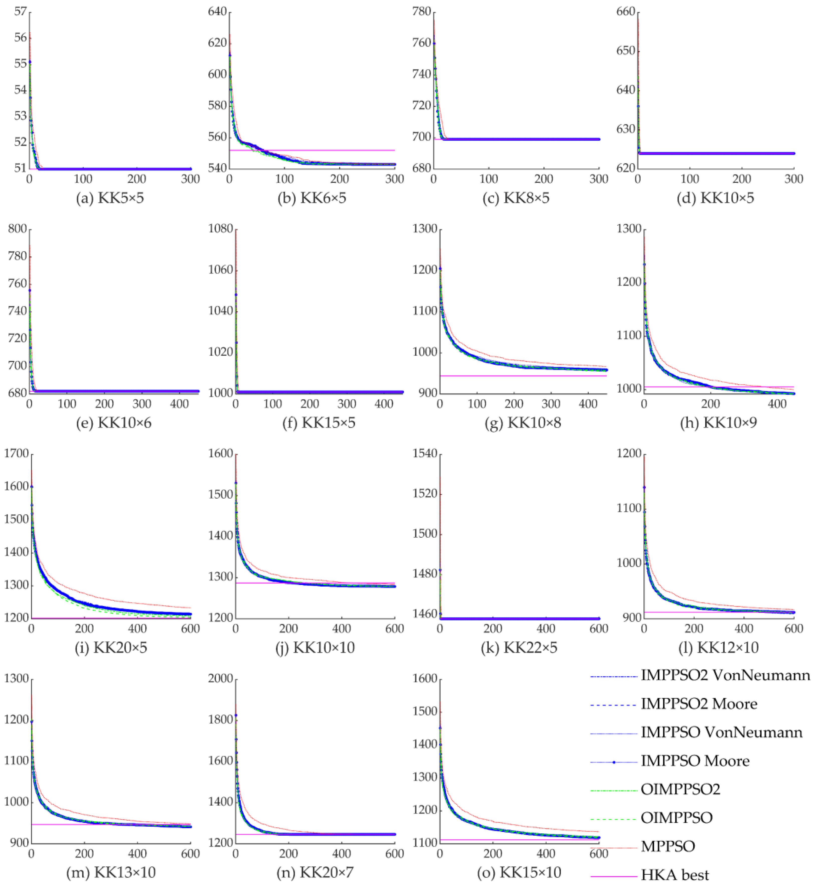
4.4. Experimental Result

The average convergence of the algorithms for the optimal solution of the Kundakcı and Kulak problem set is shown in Figure 4. The x-axis and y-axis of all subplots in Figure 4 represent the generation and fitness (time units), respectively. It can be seen from the figure that most versions of the MPPSO can converge quickly to the optimal solution of the Kundakcı and Kulak problem set obtained by the HKA algorithm. All versions of the MPPSO perform best with small-size problems, well with medium-size problems, and not very well with large-size problems. Although some benchmark instances of the Kundakcı and Kulak problem set, such as KK10 × 8, kk20 × 5, kk15 × 10, do not reach their optimal solutions obtained by the HKA algorithm, the average convergence curves of all versions of the MPPSO maintain a downward trend, which means that increasing the number of iterations can improve their performance further. The various versions of the IMPPSO have better convergence than the original MPPSO. They can converge more quickly and continue their convergence. Compared with other versions of the improved MPPSO, the algorithms with the cellular neighbor network can reduce their convergence speed, which is considered beneficial to avoid the algorithm falling into the local optimum.

Figure 5 shows the statistical analysis of the algorithms for the fitness for the Kundakcı and Kulak problem set. The x-axis and y-axis of all subplots in Figure 5 represent the algorithm and fitness (time units), respectively, the red + represents outliners. It can be seen from the figure that all versions of the MPPSO show very good robustness in 7 of 12 of the benchmark instances of the problem set. In other benchmarks, all of the improved versions of the MPPSO show better performance than the original MPPSO.

Table 4. The computational statistics of the algorithms for the fitness for some instances in the Kundakcı and Kulak problem set.

Name		KK6 × 5	KK10 × 8	KK10 × 9	KK20 × 5	KK10 × 10	KK12 × 10	KK13 × 10	KK15 × 10
IMPPSO2 VonNeumann	Min	543	935	990	1202	1268	904	933	1092
	Max	544	974	1005	1234	1292	916	948	1132
	Mean	543.03	955.10	993.43	1210.60	1278.73	909.30	941.47	1118.73
	Std.	0.18	10.17	5.58	7.33	6.31	4.27	4.04	8.71
	SR	100	16.67	100	6.67	93.33	76.67	93.33	23.33
IMPPSO2 Moore	Min	543	935	990	1191	1269	904	930	1099
	Max	544	979	1005	1232	1294	916	947	1134
	Mean	543.07	958	993.30	1212.93	1279.57	910.43	939.43	1117.87
	Std.	0.25	10.56	4.04	8.41	6.68	3.46	4.44	8.38
	SR	100	6.67	100	10	90	73.33	100	33.33
IMPPSO VonNeumann	Min	543	949	990	1192	1269	904	932	1102
	Max	544	973	1008	1225	1293	916	948	1130
	Mean	543.13	961.37	992.53	1210.90	1279.80	911.77	942.23	1117.53
	Std.	0.35	6.83	4.46	6.47	5.38	3.41	5.43	7.10
	SR	100	0	93.33	3.33	96.67	56.67	73.33	23.33
IMPPSO Moore	Min	543	936	990	1200	1268	904	930	1105
	Max	543	975	1010	1227	1287	916	948	1132
	Mean	543	958.47	992.33	1214.10	1278.53	911.70	941.23	1118.87
	Std.	0	8.10	4.90	6.43	5.64	4.26	5.12	7.40
	SR	100	3.33	96.67	3.33	100	43.33	83.33	16.67
OIMPPSO2	Min	543	940	990	1200	1269	904	930	1098
	Max	544	973	1005	1220	1292	916	949	1135
	Mean	543.07	957.73	992.37	1208.97	1278.60	911.90	942.80	1121.43
	Std.	0.25	7.26	3.52	5.59	7.32	3.35	5.17	8.99
	SR	100	3.33	100	16.67	93.33	50	76.67	10
OIMPPSO	Min	543	933	990	1192	1269	904	936	1101
	Max	543	969	1007	1213	1286	916	948	1132
	Mean	543	955.37	991.77	1204.63	1278.23	910.80	941.97	1118.50
	Std.	0	8.94	4.27	5.86	5.20	3.46	4.34	7.47
	SR	100	10	96.67	36.67	100	66.67	90	16.67
MPPSO	Min	543	948	990	1213	1270	909	939	1115
	Max	549	987	1014	1248	1294	924	955	1153
	Mean	543.23	966.67	999.80	1233.33	1283.33	916.90	948.20	1136.20
	Std.	1.10	9.22	7.33	8.80	6.50	3.44	3.57	8.72
	SR	100	0	70	0	76.67	10	30	0

shows the computational statistics of the algorithms for the fitness for some instances in the Kundakcı and Kulak problem set. The algorithms with a cellular neighbor network (IMPPSO2 VonNeumann, IMPPSO2 Moore, IMPPSO VonNeumann and IMPPSO Moore) perform better than the other versions of the improved algorithms. Furthermore, the algorithms with a cellular network perform better in large-size problems. Moreover, the Von Neumann neighborhood has better performance than the Moore neighborhood and can obtain solutions that are closer to the optimal solutions of the benchmark instances. The Von Neumann neighborhood can reduce the convergence speed of the algorithm, which is beneficial to avoid the algorithm falling into the local optimal solution and is more likely to find the global optimal solution. In large-size problems, the Von Neumann neighborhood is more likely to find better solutions for the benchmark instances. However, for a single algorithm, OIMPPSO performs the best. The IMPPSO2 shows better robustness than the IMPPSO. The IMPPSO2 can obtain the optimal solutions of the benchmark instances better than the IMPPSO.

The IMPPSO2 with the Von Neumann neighborhood obtains a better solution for the KK15 × 10 benchmark instance. The best solution of the KK15 × 10 with IMPPSO2 VonNeumann is shown in

Table 5. The best solution of the KK15 × 10 with IMPPSO2 VonNeumann.

M1	ON 1	22	13	113	133	83	103	65	154	77	98	128	46	7	150	59	40	170
	ST 2	31	125	137	195	275	353	373	431	478	571	640	713	757	810	885	980	1073
	FT 3	114	137	195	275	353	373	419	478	565	640	682	757	810	885	980	1073	1092
M2	ON	131	21	81	14	101	75	95	155	147	118	56	37	169	129	49	9	70
	ST	0	12	31	137	179	339	386	478	516	619	691	698	785	877	928	979	1000
	FT	12	31	59	179	210	384	460	516	557	691	698	785	877	923	977	1000	1091
M3	ON	91	12	32	1	73	145	163	153	104	134	43	117	85	55	69	130	29
	ST	0	94	125	212	246	285	335	396	431	448	498	596	619	656	691	923	940
	FT	94	125	212	246	285	335	396	431	448	498	596	619	656	691	750	940	1004
M4	ON	11	142	23	161	63	2	35	84	96	116	127	136	45	78	108	159	60
	ST	0	61	116	150	240	256	331	400	460	492	591	648	696	713	802	926	980
	FT	46	116	150	168	256	311	400	426	487	591	639	667	713	754	889	971	1056
M5	ON	141	31	61	72	162	102	114	125	24	19	5	44	58	139	158	100	90
	ST	0	61	121	149	169	264	288	333	431	524	579	600	726	812	906	926	1059
	FT	61	121	149	169	264	288	333	431	523	579	600	696	787	906	926	1022	1092
M6	ON	111	71	121	82	92	62	144	34	3	18	168	137	57	107	28	50	160
	ST	0	28	37	64	97	181	240	254	331	426	589	667	698	726	861	977	1002
	FT	28	37	64	97	181	240	254	331	426	524	661	695	726	802	898	1002	1080
M7	ON	151	143	53	93	74	17	115	126	166	67	25	6	138	38	48	88	110
	ST	75	127	164	181	285	339	416	492	559	564	616	678	749	812	853	928	1017
	FT	127	164	173	259	339	416	492	559	564	616	678	749	812	853	928	1017	1035
M8	ON	52	124	76	36	156	167	20	68	99	149	86	47	120	109	140	10	30
	ST	35	200	384	455	516	564	589	655	682	727	745	757	800	889	921	1019	1045
	FT	130	267	455	493	557	589	655	682	727	745	753	800	886	921	1019	1045	1088
M9	ON	51	132	41	123	152	33	16	146	164	66	97	106	119	27	87	8	80
	ST	0	35	85	173	200	224	262	339	418	452	502	571	691	799	861	927	979
	FT	35	85	164	200	224	248	339	418	452	502	571	652	781	861	927	979	993
M10	ON	112	122	54	15	64	94	42	165	4	105	135	148	26	157	39	79	89
	ST	28	125	173	183	262	305	386	463	527	543	568	648	720	799	853	936	1017
	FT	125	173	183	262	305	386	463	527	543	568	648	720	799	817	936	979	1059

¹ Operation Number; ² Start Time; ³ Finish Time.

. Figure 6 shows the Gantt chart of the KK15 × 10 with IMPPSO2 VonNeumann. Job are represented by abbreviations from J1 to J17. The machine breakdown (MB, represented by the yellow background in the figure) of machine 4 and machine 8 occurs during the processing of job 2 and job 13, respectively.

Figure 7 shows the statistical analysis of the algorithms for the running time for the Kundakcı and Kulak problem set. The x-axis and y-axis of all subplots in Figure 7 represent the algorithm and running time (s), respectively, where red + represents outliners. All of the improved MPPSOs run longer than the original MPPSO, essentially doubling the time. However, the running time of all of the improved MPPSOs are almost the same. For small-size problems, the average time for 30 independent runs of all of the improved algorithms is within 30 s. The average time for 30 independent runs of almost all of the improved algorithms is within 2 min for medium-size problems. For large-size problems, the average time for 30 independent runs of all of the improved algorithms is within 4 min for most benchmark instances and within 6 min for only two of the benchmark instances. Therefore, as the problem size increases, the algorithm running time increases significantly. However, the running times of the algorithms are acceptable, which gives a suboptimal solution for the problem in a reasonable time.

5. Case Study

The operation of the proposed algorithm in a real-world environment is studied using a simulation model of a production system for the evaluation of dynamic events’ impacts. The simulation modelling is performed using Simio software. According to the previously proposed data transfer architecture between the decision algorithm and the simulation model (MatLab to Simio data transfer) [36], we conduct an experiment in which we observe the influence of dynamic events on the production system’s productivity and its efficiency. We focus on analyzing the correctness of the proposed decision-making algorithm’s (IMPPSO) operation using five representative parameters of the production system’s efficiency (machine utilization, machine time processing, machine breakdown time, machine operational costs, and machine breakdown costs). With the help of the simulation model and the given results, we are able to confirm the adequacy of the operation and the applicability of the proposed method.

5.1. Case Description

Figure 8 shows a simulation model of a manufacturing plant in the European Union where we have twelve workstations (machines from M1 to M12) and two additional stations: the arrival and dispatch of orders station. The simulation model and its entities summarize the characteristics of a real-world production system; the simulation model was built for the testing purposes of the proposed algorithm, and it can be used in everyday production scheduling tasks. The data of the real-world production system present the input data to the simulation model, where we have a known number of initial orders, a known order sequence, and the expected processing time of the individual operation on a specific needed machine. Dynamic events, which are not known in advance, and on the basis of which the decision IMPPSO algorithm must react in real-time, include a change in the estimated processing time of the operation, the arrival of a new order, and the breakdown of the machine. A fast response to dynamic events allows the production system to function in a timely and financially justified manner. The simulation time assumes the execution of job orders corresponding to the boundary conditions of the model: The production use a two-hour warm-up period, the paths between the machining centers are without lengths (the transport is carried out by a forklift), each workstation is operated by an operator, the entered series of orders is ready for machining at the start time, and the finished orders are dispatched immediately in the shipping process. The characteristics of the workstation operation are assumed according to the DJSSP literature, the details of which were presented in the second section.

The input data set and associated dynamic events are shown in

Table 6. Real-world simulation model input parameters.

Jobs	Occurrence Time	Machine Sequence	Processing Time [Time Unit]	Dynamic Event
J1	0	M1, M4, M8, M9, M10, M12	139
J2	0	M1, M5, M7, M9, M11, M12	121
J3	0	M9, M10, M12	52	Change in the process time to 50
J4	0	M2, M4, M8, M9, M11, M12	139
J5	0	M2, M6, M8, M9, M10, M12	137
J6	0	M1, M5, M7, M9, M11, M12	121
J7	0	M2, M4, M8, M9, M11, M12	139
J8	0	M2, M6, M7, M9, M10, M12	146	Change in the process time to 149
J9	0	M1, M3, M7, M9, M11, M12	123
J10	0	M1, M5, M7, M9, M11, M12	121
J11	0	M1, M5, M7, M9, M11, M12	126
J12	0	M2, M3, M8, M9, M11, M12	139
J13	0	M1, M5, M7, M9, M11, M12	124
J14	0	M1, M6, M7, M9, M10, M12	139
J15	0	M9, M10, M12	50
J16	125	M1, M4, M8, M9, M10, M12	139	New job arrival
J17	155	M1, M5, M7, M9, M11, M12	125	New job arrival
0	50	M2	7	Machine breakdown
0	175	M9	5	Machine breakdown

. The displayed set of orders assumes three different types of dynamic events (a change in the process time of a specific job, a new job arrival, and an unknown machine breakdown) in as many as 35% of the orders. High-order dynamics and the tracking of the optimal utilization of the production system are only possible if the proposed IMPPSO algorithm is used and the decision making is done in real-time. The performance of the production system with the indicated dynamics of orders and events prevents the optimal operation and global competitiveness of the company or represents its high risk.

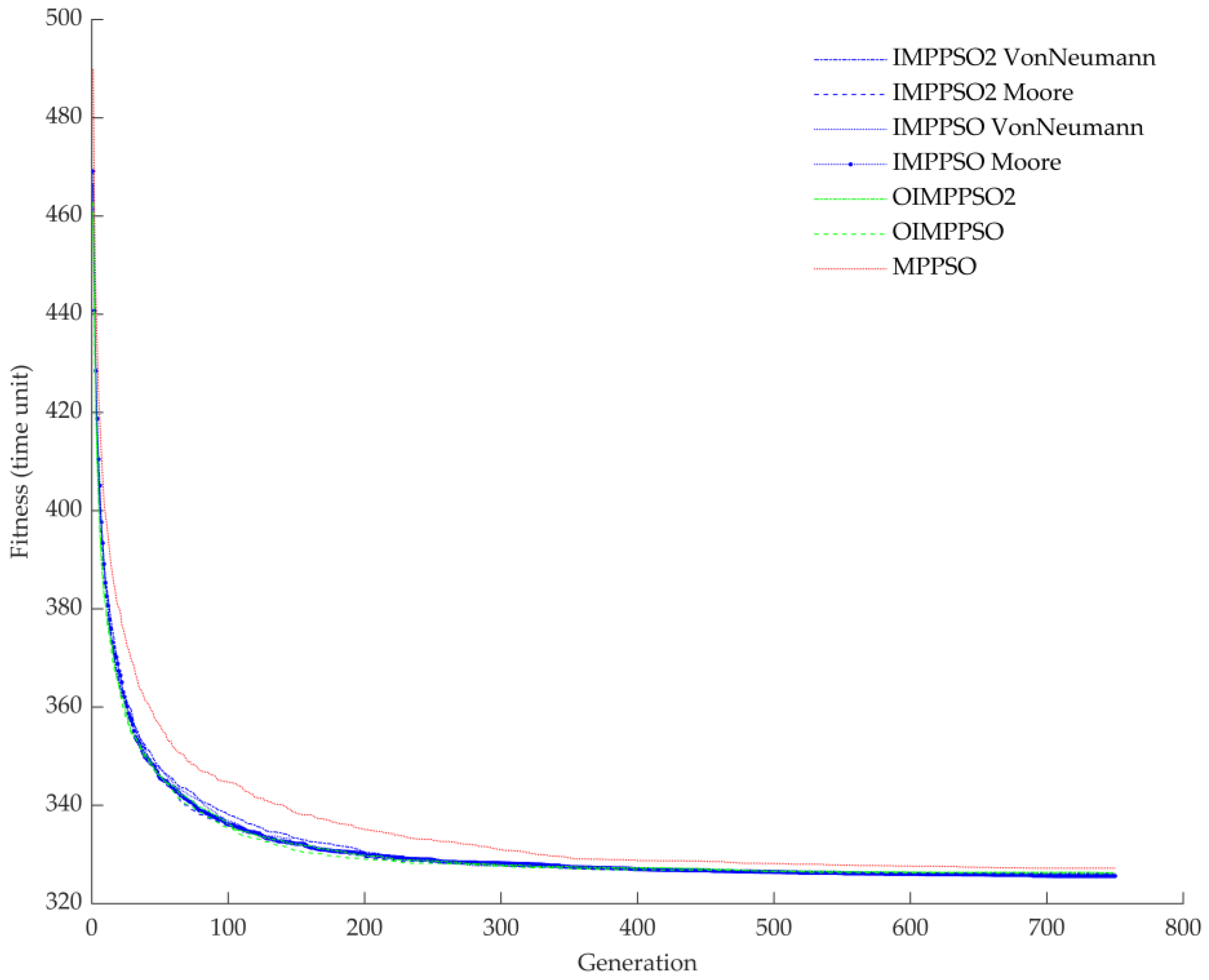
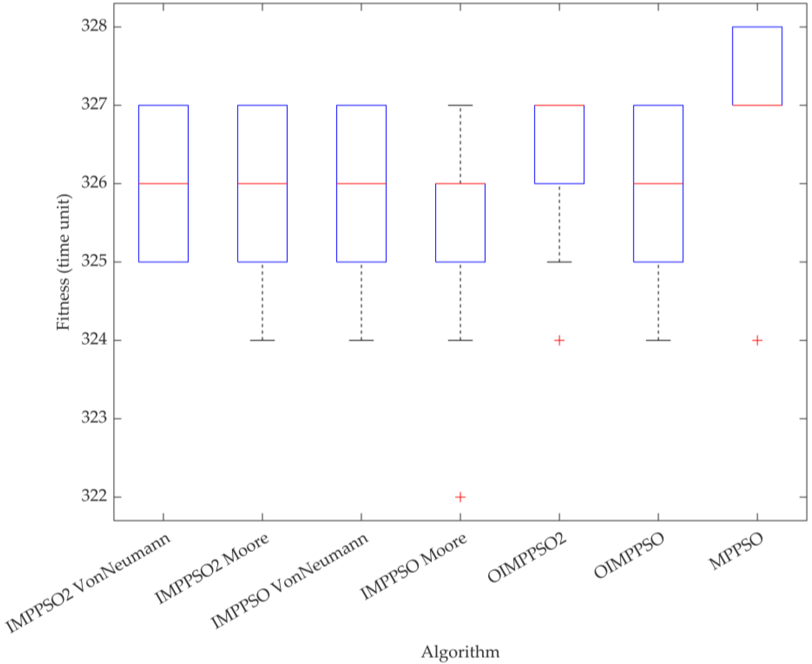
5.2. Algorithm Experiment

Because the number of jobs and the number of machines for the case are 15 and 12, respectively, and based on experiments, the maximum number of iterations for all versions of the MPPSO is set to 750, and the other parameters are the same as in Table 3. The average convergence of the algorithms for the optimal solution of the case is shown in Figure 9. It can also be seen that the various versions of the IMPSSO increase the convergence speed and improve the performance, and the various versions of the IMPSSO with the cellular neighbor structures can reduce its convergence speed appropriately and improve the performance further.

Figure 10 shows the statistical analysis of the algorithms for the fitness of the case, where red + represents outliners. It can also be seen that the various versions of the IMPPSO have better statistical performance, and the performance of the IMPPSO with the cellular neighbor structures is further improved.

The IMPPSO with the Moore neighborhood obtains a better solution for the case. Figure 11 shows the Gantt chart of jobs from J1 to J17, with the machine brake down (MB), of the case with IMPPSO Moore. The breakdown of machine 2 occurs during the processing of job 4, while a machine breakdown occurs when machine 9 happens to be idle.

Figure 12 shows the statistical analysis of the algorithms for the running time of the case, where red + represents outliner. It can also be seen that the running time of various versions of the IMPPSO is basically twice that of the original MPPSO, while the running times of various versions of the IMPPSO are basically the same.

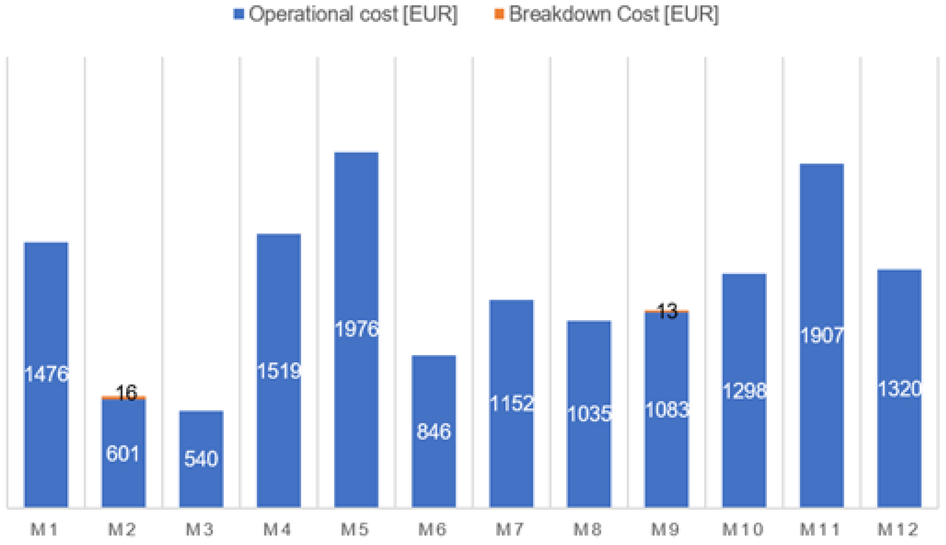
5.3. Simulation Modelling Result

The simulation result in

Table 7. The results of the simulation model.

Machine	Machine Time Processing [Time Unit]	Machine Utilization [%]	Operational Cost [EUR]
M1	206	100	1476
M2	103	100	601
M3	83	45.6	540
M4	172	91.9	1519
M5	228	98.3	1976
M6	86	92.1	846
M7	192	87.7	1152
M8	138	82.6	1035
M9	171	71.5	1083
M10	173	64.8	1298
M11	220	99.5	1907
M12	220	77.7	1320

shows three observed parameters (machine time processing, machine utilization, and machine operational cost) describing the operation of the production system and the effects of the dynamic events. The average machine processing time is a 166 time unit with a standard deviation of a 50.1 time unit. The value of the standard deviation proves the adequacy of the simulation model operation and the IMPPSO algorithm, as the machine processing times are correlated with the input data set, in which the production system processes real-world products, where the normative times of individual operations vary depending on the necessary execution of the technological process. Since the problem involves DJSSP and dynamic events, in which machine breakdown plays a crucial role, the parameter machine downtime is also plotted in Figure 13, where the results are consistent with the input data presented in Table 6. The high performance of the proposed IMPPSO algorithm is demonstrated by the simulation modelling results of the machine utilization rate, as this value is, on average, 84.3%, which, according to the literature [5] and the properties of the DJSSP problem, proves the high efficiency of the proposed algorithm. The standard deviation of the machine utilization parameter is 16.2%, where we note in a detailed analysis that the size of the deviation depends on the number of operations that need to be performed on a given machine, as well as the possible waiting time until the arrival of a new order appears. Based on the results, we note that a larger number of orders would improve the machine utilization rate parameter further.

Considering the global market dynamics, when the justification of production systems is conditioned primarily by the operation cost evaluation, Table 7 and Figure 14 show the operational and breakdown costs. The presented results show the importance of reducing the number of unscheduled machines’ breakdowns, but, when they occur, the IMPPSO algorithm must reschedule orders successfully and propose a new execution of individual operations on specific machines in real-time. In the present case, it is shown that the proposed algorithm can distribute individual operations optimally to the appropriate machines while reducing the machine breakdown time (and, hence, the cost), as shown in Figure 14. Downtime-related failures in the case study example account for only 0.2% of the total operation value in the production system.

6. Discussion

In all benchmark instances of the Kundakcı and Kulak problem set, all improved MPPSO versions converge faster than the original MPPSO while maintaining their performance. The randomly select sub-dimension strategy is the key factor. Moreover, this is the reason why their run times for all benchmark instances increase significantly. The introduction of the cellular neighbor network can reduce the convergence speed of the improved algorithms, which is most obvious in KK20 × 5. Decreasing the speed of convergence is considered to be beneficial to increase the global exploration capability of the algorithm. The global exploration capability of the IMPPSO2 is better than that of the IMPPSO, which is more likely to find the global optimal solution. When reinitializing the velocity of a particle, reinitializing the velocity randomly can enhance the diversity of the population.

The IMPPSO can obtain a solution that is closer to the real optimal solution of each benchmark instance of the Kundakcı and Kulak problem set. The improvement of algorithms for the optimal solution of the Kundakcı and Kulak problem set is shown in

Table 8. The improvement of the IMPPSO for the optimal solution of the Kundakcı and Kulak problem set.

Size Type	No	Name	GAM Best	HKA Best	IMPPSO Best	Improvement Rate for GAM (%)	Improvement Rate for HKA (%)
small	1	KK5 × 5	51	51	51	0	0
	2	KK6 × 5	557	552	543	2.51	1.63
	3	KK8 × 5	699	699	699	0	0
	4	KK10 × 5	624	624	624	0	0
medium	5	KK10 × 6	682	682	682	0	0
	6	KK15 × 5	1001	1001	1001	0	0
	7	KK10 × 8	1027	944	933	9.15	1.17
	8	KK10 × 9	1049	1005	990	5.62	1.49
large	9	KK20 × 5	1361	1202	1191	12.49	0.92
	10	KK10 × 10	1389	1287	1268	8.71	1.48
	11	KK22 × 5	1458	1458	1458	0	0
	12	KK12 × 10	1002	912	904	9.78	0.88
	13	KK13 × 10	1016	947	930	8.46	1.80
	14	KK20 × 7	1326	1246	1246	6.03	0
	15	KK15 × 10	1280	1112	1092	14.69	1.80

. Compared with the GAM, the IMPPSO has improved fitness for most benchmark instances of the Kundakcı and Kulak problem set, which has the most obvious effect in large-size problems. Compared with the GAM, the average improvement rate of the IMPPSO is 5.16%, the minimum improvement rate is 2.51%, and the maximum improvement rate is 14.69%. Similarly, the IMPPSO further improves the fitness for most of the benchmark instances of the Kundakcı and Kulak problem set obtained by the HKA, which also has the most obvious effect in large-size problems. Compared with the HKA, the average improvement rate of the IMPPSO is 0.74%, the minimum improvement rate is 0.88%, and the maximum improvement rate is 1.80%. Therefore, the IMPPSO has better global exploration capability than the GAM and HKA, which can find a suboptimal solution that is closer to the optimal solution of each benchmark instance of the Kundakcı and Kulak problem set. Compared with the GAM and HKA, the IMPPSO improves the fitness of the benchmark instances of the Kundakcı and Kulak problem set by 60% and 53.33%, respectively.

The various versions of MPSSO are used in the case study. The various versions of the IMPPSO, especially those with the cellular neighbor structures, achieve relatively good performance. However, their performance in obtaining the true optimal solution of the case still needs to be improved further, for the real-world problems are more complex. We can see from the case that a job does not need to be processed on all machines, resulting in further discretization of the solution space, and more local extrema may appear, which will increase the difficulty of solving the problem further. The advantages of the proposed decision-making algorithm can also be seen in the result of the simulation model, which proves that the presented algorithm enables the scheduling of orders and dynamic events’ decision-making, so that the production system operates in the optimal mode. The successful implementation of the proposed IMPPSO algorithm in the commercial software package Simio is possible, as stated in the literature [36,37], but, unlike in the literature, the presented simulation model allows the monitoring of the dynamic events of the DJSSP problem. The advantage of the case study evaluation is the real-world input data, which allow evaluation of both the decision-making algorithm and the simulation model. In the future, it is necessary to generate and obtain more extensive and complex data sets to improve and optimize the performance of both the decision-making algorithm and the simulation model further.

7. Conclusions

The IMPPSO is proposed by introducing the cellular neighbor network, the velocity reinitialization strategy, the randomly select sub-dimension strategy, and the constraint- handling function. The Von Neumann neighborhood and the Moore neighborhood are introduced in the cellular neighbor network. The velocity reinitialization strategy uses a linear dynamic velocity change variable. The strategy is adopted by selecting sub-dimensions randomly from the remaining dimensions that have not been updated. The constraint handling function, which assigns the violated dimension to a random value, a global optimal value or a boundary value with a certain probability, is introduced to handle constraints. The MPPSO and HKA are selected as a comparison of various versions of the IMPPSO. The various versions of the IMPPSO have faster convergence and better global exploration capability. While requiring twice as much running time as the original MPPSO, they can obtain suboptimal solutions for the problem in a reasonable time. The average improvement rate in the fitness of the IMPPSO for the benchmark instances of the Kundakcı and Kulak problem set is 5.16% compared to the GAM and 0.74% compared to the HKA.

The performance of the various versions of the IMPPSO applied to solve real-world problems is verified by a case study. The various versions of the IMPPSO perform better than the original MPPSO. Due to the complexity of real-world problems, the performance of the IMPPSO needs to be improved further. The importance of the presented work is reflected in the daily consideration of the DJSSP production system scheduling, where dynamic events pose increasing challenges to the industry. The integration of the presented decision-making algorithm and the simulation model, which can be applied in the daily scheduling practice, enables the rapid adaptation of the production system to dynamic events. The possibility of using the presented method enables rapid adaptation to other dynamic events, which are occurring increasingly in times of pandemics, tightened security problems, and unreliable supply chains.

The presented results indicate a diverse spectrum of further research that will focus on optimizing the proposed IMPPSO algorithm’s efficiency, where we will work to ensure a high level of efficiency and robustness of the algorithm’s operation for small, medium, and large datasets. Further research of the proposed simulation model with a comparative study of multiple algorithms would confirm the strong potential of the proposed algorithm, as proven in the decision-making algorithm comparison. As stated in the literature [16,19], it is not possible to trace the interconnectivity between an effective decision-making and simulation model solving DJSSP, which can be stated as one of the advantages of the presented work.

References

1. Ramasesh, R. Dynamic Job Shop Scheduling: A Survey of Simulation Research. Omega 1990, 18, 43–57. [Google Scholar] [CrossRef]
2. Hinderer, K.; Rieder, U.; Stieglitz, M. Introduction and Organization of the Book. In Dynamic Optimization; Universitext; Springer International Publishing: Cham, Switzerland, 2016; pp. 1–11. ISBN 978-3-319-48813-4. [Google Scholar]
3. Park, J.; Mei, Y.; Nguyen, S.; Chen, G.; Zhang, M. An Investigation of Ensemble Combination Schemes for Genetic Programming Based Hyper-Heuristic Approaches to Dynamic Job Shop Scheduling. Appl. Soft Comput. 2018, 63, 72–86. [Google Scholar] [CrossRef]
4. Wang, Z.; Zhang, J.; Yang, S. An Improved Particle Swarm Optimization Algorithm for Dynamic Job Shop Scheduling Problems with Random Job Arrivals. Swarm Evol. Comput. 2019, 51, 100594. [Google Scholar] [CrossRef]
5. Chryssolouris, G.; Subramaniam, V. Dynamic Scheduling of Manufacturing Job Shops Using Genetic Algorithms. J. Intell. Manuf. 2001, 12, 281–293. [Google Scholar] [CrossRef]
6. Zhang, L.; Gao, L.; Li, X. A Hybrid Genetic Algorithm and Tabu Search for a Multi-Objective Dynamic Job Shop Scheduling Problem. Int. J. Prod. Res. 2013, 51, 3516–3531. [Google Scholar] [CrossRef]
7. Nguyen, S.; Zhang, M.; Johnston, M.; Tan, K.C. Automatic Design of Scheduling Policies for Dynamic Multi-Objective Job Shop Scheduling via Cooperative Coevolution Genetic Programming. IEEE Trans. Evol. Comput. 2014, 18, 193–208. [Google Scholar] [CrossRef]
8. Aydin, M.E.; Öztemel, E. Dynamic Job-Shop Scheduling Using Reinforcement Learning Agents. Rob. Auton. Syst. 2000, 33, 169–178. [Google Scholar] [CrossRef]
9. Shahrabi, J.; Adibi, M.A.; Mahootchi, M. A Reinforcement Learning Approach to Parameter Estimation in Dynamic Job Shop Scheduling. Comput. Ind. Eng. 2017, 110, 75–82. [Google Scholar] [CrossRef]
10. Shen, X.-N.; Yao, X. Mathematical Modeling and Multi-Objective Evolutionary Algorithms Applied to Dynamic Flexible Job Shop Scheduling Problems. Inf. Sci. 2015, 298, 198–224. [Google Scholar] [CrossRef]
11. Baykasoğlu, A.; Madenoğlu, F.S.; Hamzadayı, A. Greedy Randomized Adaptive Search for Dynamic Flexible Job-Shop Scheduling. J. Manuf. Syst. 2020, 56, 425–451. [Google Scholar] [CrossRef]
12. Zhang, F.; Mei, Y.; Nguyen, S.; Zhang, M. Evolving Scheduling Heuristics via Genetic Programming With Feature Selection in Dynamic Flexible Job-Shop Scheduling. IEEE Trans. Cybern. 2021, 51, 1797–1811. [Google Scholar] [CrossRef]
13. Zhou, Y.; Yang, J.-J.; Huang, Z. Automatic Design of Scheduling Policies for Dynamic Flexible Job Shop Scheduling via Surrogate-Assisted Cooperative Co-Evolution Genetic Programming. Int. J. Prod. Res. 2020, 58, 2561–2580. [Google Scholar] [CrossRef]
14. Nie, L.; Gao, L.; Li, P.; Li, X. A GEP-Based Reactive Scheduling Policies Constructing Approach for Dynamic Flexible Job Shop Scheduling Problem with Job Release Dates. J. Intell. Manuf. 2013, 24, 763–774. [Google Scholar] [CrossRef]
15. Zhang, M.; Tao, F.; Nee, A.Y.C. Digital Twin Enhanced Dynamic Job-Shop Scheduling. J. Manuf. Syst. 2021, 58, 146–156. [Google Scholar] [CrossRef]
16. Kuck, M.; Ehm, J.; Hildebrandt, T.; Freitag, M.; Frazzon, E.M. Potential of Data-Driven Simulation-Based Optimization for Adaptive Scheduling and Control of Dynamic Manufacturing Systems. In Proceedings of the 2016 Winter Simulation Conference (WSC), Washington, DC, USA, 11–14 December 2016; pp. 2820–2831. [Google Scholar]
17. Zhou, L.; Zhang, L.; Ren, L.; Wang, J. Real-Time Scheduling of Cloud Manufacturing Services Based on Dynamic Data-Driven Simulation. IEEE Trans. Ind. Inform. 2019, 15, 5042–5051. [Google Scholar] [CrossRef]
18. Yang, W.; Takakuwa, S. Simulation-Based Dynamic Shop Floor Scheduling for a Flexible Manufacturing System in the Industry 4.0 Environment. In Proceedings of the 2017 Winter Simulation Conference (WSC), Las Vegas, NV, USA, 3–6 December 2017; pp. 3908–3916. [Google Scholar]
19. Ojstersek, R.; Buchmeister, B. Simulation Based Resource Capacity Planning with Constraints. Int. J. Sim. Model. 2021, 20, 672–683. [Google Scholar] [CrossRef]
20. Vinod, V.; Sridharan, R. Simulation-Based Metamodels for Scheduling a Dynamic Job Shop with Sequence-Dependent Setup Times. Int. J. Prod. Res. 2009, 47, 1425–1447. [Google Scholar] [CrossRef]
21. Vinod, V.; Sridharan, R. Simulation Modeling and Analysis of Due-Date Assignment Methods and Scheduling Decision Rules in a Dynamic Job Shop Production System. Int. J. Prod. Econ. 2011, 129, 127–146. [Google Scholar] [CrossRef]
22. Xiong, H.; Fan, H.; Jiang, G.; Li, G. A Simulation-Based Study of Dispatching Rules in a Dynamic Job Shop Scheduling Problem with Batch Release and Extended Technical Precedence Constraints. Eur. J. Oper. Res. 2017, 257, 13–24. [Google Scholar] [CrossRef]
23. Zou, J.; Chang, Q.; Arinez, J.; Xiao, G.; Lei, Y. Dynamic Production System Diagnosis and Prognosis Using Model-Based Data-Driven Method. Expert Syst. Appl. 2017, 80, 200–209. [Google Scholar] [CrossRef]
24. Jemmali, M.; Hidri, L.; Alourani, A. Two-stage Hybrid Flowshop Scheduling Problem With Independent Setup Times. Int. J. Sim. Model. 2022, 21, 5–16. [Google Scholar] [CrossRef]
25. Kundakcı, N.; Kulak, O. Hybrid Genetic Algorithms for Minimizing Makespan in Dynamic Job Shop Scheduling Problem. Comput. Ind. Eng. 2016, 96, 31–51. [Google Scholar] [CrossRef]
26. Heppner, F.; Grenander, U. A Stochastic Nonlinear Model for Coordinated Bird Flocks. In The Ubiquity of Chaos; Krasner, S., Ed.; AAAS Publications: Washington, DC, USA, 1990; pp. 233–238. [Google Scholar]
27. Kennedy, J.; Eberhart, R. Particle Swarm Optimization. In Proceedings of the Proceedings of ICNN’95—International Conference on Neural Networks, Perth, Australia, 27 November–1 December 1995; Volume 4, pp. 1942–1948. [Google Scholar]
28. Al-Kazemi, B.S.N. Multiphase Particle Swarm Optimization; Syracuse University: New York, NY, USA, 2002. [Google Scholar]
29. Zhang, H. Research on Multi-Objective Swarm Intelligence Algorithms for Door-to-Door Railway Freight Transportation Routing Design; Beijing Jiaotong University: Beijing, China, 2019. [Google Scholar]
30. Zhang, H.; Buchmeister, B.; Li, X.; Ojstersek, R. Advanced Metaheuristic Method for Decision-Making in a Dynamic Job Shop Scheduling Environment. Mathematics 2021, 9, 909. [Google Scholar] [CrossRef]
31. Li, X.-Y.; Yang, L.; Li, J. Dynamic Route and Departure Time Choice Model Based on Self-Adaptive Reference Point and Reinforcement Learning. Phys. A Stat. Mech. Its Appl. 2018, 502, 77–92. [Google Scholar] [CrossRef]
32. Wikipedia Von Neumann Neighborhood. Available online: https://en.wikipedia.org/wiki/Von_Neumann_neighborhood (accessed on 26 August 2020).
33. Wikipedia Moore Neighborhood. Available online: https://en.wikipedia.org/wiki/Moore_neighborhood (accessed on 23 June 2022).
34. Sha, D.Y.; Lin, H.-H. A Multi-Objective PSO for Job-Shop Scheduling Problems. Expert Syst. Appl. 2010, 37, 1065–1070. [Google Scholar] [CrossRef]
35. Marinakis, Y.; Marinaki, M. A Hybrid Particle Swarm Optimization Algorithm for the Open Vehicle Routing Problem. In Swarm Intelligence, Proceedings of the 8th International Conference, ANTS 2012, Brussels, Belgium, 12–14 September 2012; Dorigo, M., Birattari, M., Blum, C., Christensen, A.L., Engelbrecht, A.P., Groß, R., Stützle, T., Eds.; Springer: Berlin/Heidelberg, Germany, 2012; pp. 180–187. ISBN 978-3-642-32650-9. [Google Scholar]
36. Ojstersek, R.; Lalic, D.; Buchmeister, B. A New Method for Mathematical and Simulation Modelling Interactivity: A Case Study in Flexible Job Shop Scheduling. Adv. Prod. Eng. Manag. 2019, 14, 435–448. [Google Scholar] [CrossRef]
37. Guzman, E.; Andres, B.; Poler, R. A Decision-Making Tool for Algorithm Selection Based on a Fuzzy TOPSIS Approach to Solve Replenishment, Production and Distribution Planning Problem. Mathematics 2022, 10, 1544. [Google Scholar] [CrossRef]
Figure 1. The flowchart of the MPPSO.
Mathematics 11 02336 g001
Figure 2. The examples of cellular neighborhoods and cellular neighbor networks.
Mathematics 11 02336 g002
Figure 3. An example of the encoding solution.
Mathematics 11 02336 g003
Figure 4. The average convergence of the algorithms for the optimal solution of the Kundakcı and Kulak problem set.
Mathematics 11 02336 g004
Figure 5. The statistical analysis of the algorithms for the fitness for the Kundakcı and Kulak problem set.
Mathematics 11 02336 g005
Figure 6. The Gantt chart of the KK15 × 10 with IMPPSO2 VonNeumann.
Mathematics 11 02336 g006
Figure 7. The statistical analysis of the algorithms for the running time of the Kundakcı and Kulak problem set.
Mathematics 11 02336 g007
Figure 8. The simulation model in Simio Software.
Mathematics 11 02336 g008
Figure 9. The average convergence of the algorithms for the optimal solution of the case.
Mathematics 11 02336 g009
Figure 10. The statistical analysis of the algorithms for the fitness of the case.
Mathematics 11 02336 g010
Figure 11. The Gantt chart of the case with IMPPSO Moore.
Mathematics 11 02336 g011
Figure 12. The statistical analysis of the algorithms for the running time of the case.
Mathematics 11 02336 g012
Figure 13. The graphical representation of the results of the simulation model.
Mathematics 11 02336 g013
Figure 14. The operational and breakdown costs.
Mathematics 11 02336 g014