CTOA: Toward a Chaotic-Based Tumbleweed Optimization Algorithm

Abstract

Metaheuristic algorithms are an important area of research in artificial intelligence. The tumbleweed optimization algorithm (TOA) is the newest metaheuristic optimization algorithm that mimics the growth and reproduction of tumbleweeds. In practice, chaotic maps have proven to be an improved method of optimization algorithms, allowing the algorithm to jump out of the local optimum, maintain population diversity, and improve global search ability. This paper presents a chaotic-based tumbleweed optimization algorithm (CTOA) that incorporates chaotic maps into the optimization process of the TOA. By using 12 common chaotic maps, the proposed CTOA aims to improve population diversity and global exploration and to prevent the algorithm from falling into local optima. The performance of CTOA is tested using 28 benchmark functions from CEC2013, and the results show that the circle map is the most effective in improving the accuracy and convergence speed of CTOA, especially in 50D.

1. Introduction

As science and technology continue to advance and production capacity improves, the complexity of optimization problems is increasing. Finding efficient solution algorithms for these complex problems has become an urgent issue to be addressed. The emergence of metaheuristic algorithms provides a promising approach to solving optimization problems [1]. They are inspired by natural evolutionary laws, which have been shaped over tens of thousands of years to improve survival and to ensure that populations evolve.

Researchers have investigated these natural phenomena and designed algorithms to solve complex problems. The optimization problem is abstracted into the optimal solution of population evolution in this algorithm, the space of numerical search is abstracted into the living environment, and the behavior of each individual in the population represents a set of solutions. By continuously evolving the biological characteristics of its own population from an initial state, an optimal solution can be obtained, such as particle swarm optimization (PSO) [2], genetic algorithm (GA) [3], whale optimization algorithm (WOA) [4], grey wolf optimizer (GWO) [5], salp swarm algorithm (SSA) [6], ant colony optimization (ACO) [7], or shuffled frog leaping algorithm (SFLA) [8]. These efficient and robust algorithms have been successfully applied to solve various problems such as complex engineering problems [9,10,11], neural network [12,13,14,15], shortest path optimization [16,17], feature selection [18,19,20], and power scheduling [21].

Although metaheuristic algorithms can solve optimization problems in large-scale search spaces, Sheikholeslami et al. [22] showed that a sufficiently random sequence is required to ensure better performance in the algorithm’s global search phase, especially for metaheuristic algorithms that simulate and make decisions for complex natural phenomena. Population initialization is a critical component of metaheuristic algorithms. It has a direct impact on the algorithm’s search efficiency and the quality of the final solution. As a result, researchers have been investigating various methods to improve population initialization in order to solve practical problems more effectively. Randomized initialization is one of the most common metaheuristic initialization methods, in which a population is built by randomly generating solutions in the search space. This method is used by the majority of algorithms, such as those in [23,24]. THe initialization of opposition-based learning (OBL) randomly generates a set of solutions as the initial population and then generates an opposite solution, such as in [25,26]. Cluster-based initialization is a method that uses a clustering algorithm to divide the solutions. These solutions with similar patterns are assigned into several categories [27], such as in [28,29]. The use of chaotic maps is one of the most effective ways to generate a sufficiently random and well-distributed initialization sequence for metaheuristic algorithms, such as in [30,31,32,33]. By combining chaotic maps and metaheuristic algorithms, various optimization problems have been improved. For example, Gandomi et al. [34] proposed a chaos-accelerated particle swarm algorithm in 2013, and Arora et al. [35] proposed using chaos to improve the butterfly algorithm in 2017. The above-mentioned studies have obtained good experimental results. Kohli et al. [36] proposed a chaotic gray wolf optimization algorithm for constrained problems, and experiments proved that this method is very effective. Jia et al. [37] applied chaos theory to differential evolution and proved the feasibility of a chaotic local search strategy.

The tumbleweed optimization algorithm (TOA) [38] is a newly proposed metaheuristic algorithm inspired by the growth and reproduction behavior of tumbleweeds. Here are several existing research gaps and our motivations in this study:

• Currently, no studies focus on chaotic-based TOA algorithms. Previous studies have shown that by combining chaotic maps with metaheuristic algorithms, various optimization problems have been improved. Thus, to the best of our knowledge, we propose a chaotic-based tumbleweed optimization algorithm (named CTOA).
• In order to obtain the best performance of CTOA, we verify 12 chaotic maps. In our experiments, CEC2013, Friedman ranking test, and Wilcoxon test are adopted. Meanwhile, a real problem–power generation prediction is involved for evaluation.

Therefore, the main contributions of this paper are as follows:

• In this study, we combine chaotic maps with the TOA algorithm for the first time to propose a chaotic-based tumbleweed optimization algorithm (CTOA).
• We select 12 different chaotic maps and 28 popular benchmark functions to evaluate the performance of the proposed CTOA algorithm. The experimental results demonstrate that the performance and convergence of CTOA are greatly enhanced. We conclude that the best CTOA algorithm is CTOA9 (circle map + TOA).
• Finally, we compare CTOA9 with famous state-of-art optimization algorithms, including GA [3], PSO [2], ACO [7], and SFLA [8]. The results demonstrate that CTOA9 is not only the best in the Friedman ranking test and Wilcoxon test, but it also has the minimum error when applied to power generation prediction problems.

The remainder of this paper is structured as follows: In Section 2, a literature review is provided to summarize the existing research on chaotic-based metaheuristic optimization algorithms. We present the CTOA, which integrates twelve selected chaotic maps into TOA in Section 3. The experimental evaluation of the CTOA on a range of benchmark functions is presented in Section 4. Section 5 provides a detailed application of real problem–power generation prediction. The discussion is described in Section 6 and the conclusion is described in Section 7.

2. Related Work

One area of interest in recent years has been the use of chaotic map strategies to enhance metaheuristic algorithms. Several studies have explored the use of chaotic maps to improve the performance of metaheuristic algorithms. In 2018, Sayed et al. [39] proposed a new chaotic multi-variate optimization algorithm (CMVO) to overcome the problems of low convergence speed and local optimum in MVO. To help control the rate of exploration and exploitation, ten well-known chaotic maps were selected for their research. Experimental results show that the sinusoidal map can significantly improve the performance of the original MVO. Similarly, Du et al. [40], in 2018, proposed the use of linear decreasing and a logical chaotic map to enhance the fruit fly algorithm, named DSLC-FOA, which produced better results than the original FOA and other metaheuristic algorithms.

Tharwat et al. [41], in 2019, developed a chaotic particle swarm optimization (CPSO) to optimize path planning and demonstrated its high accuracy by adjusting multiple variables in a Bezier curve-based path planning model. Kaveh et al. [42] proposed a Gauss map-based chaotic firefly algorithm (CGFA). Experimental results show that chaotic maps can improve convergence and prevent the algorithm from getting stuck in locally optimal solutions. In 2020, Demidova et al. [43] applied two strategies of different chaotic maps with symmetric distribution and exponential step decay to the fish school search optimization algorithm (FSS) to solve the shortcomings of poor convergence speed of FSS and low precision in high-dimensional optimization problems. Ultimately, the results of the study showed that FSS using tent map produced the most accurate results. Similar to this study, Li et al. [44] also proved that the chaotic whale optimization algorithm generated by the tent map when improving the WOA has higher accuracy in numerical simulation.

In 2021, Agrawal et al. [45] used chaotic maps to improve the gaining sharing knowledge-based optimization algorithm (GSK) and applied this new algorithm to feature selection. The results indicate that the Chebyshev map shows the best result among all chaotic maps, improving the original algorithm’s performance accuracy and convergence speed. In 2022, Li et al. [46] proposed the chaotic arithmetic optimization algorithm (CAOA). The CAOA based on chaotic disturbance factors has the advantage of balancing exploration and exploitation in the optimization process. Onay et al. [47] applied ten chaotic maps to the classic hunger games search (HGS), and they were also evaluated on the classic benchmark problems in CEC2017.

Recently, Yang et al. [48] used the tent map to improve the population diversity of WOA [4]. They also optimized the parameters and network size of the radial basis function neural network (RBFNN). Luo et al. [49] proposed an improved bald eagle algorithm that combined with the tent map and Levy fight method. This improved algorithm can expand the diversity of the population and search space. Naik et al. [50] introduced chaos theory into the modification of the social group optimization (SGO) algorithm, by replacing constant values with chaotic maps. The chaotic social group optimization algorithm proposed by them improves its convergence speed and results in precision.

In summary, the use of chaotic map strategies has shown promise in improving the performance of various metaheuristic algorithms. The selection of a suitable chaotic map for a given optimization algorithm can lead to a significant improvement in its convergence speed and precision. The summaries of these studies are shown in Table 1. The potential of chaotic map strategies in improving optimization algorithms remains an active area of research, and further studies are necessary to explore their effectiveness in different optimization problems.

Table 1. Literature summary of optimization algorithms improved by a chaotic map.

Literature	Chaotic Map + Metaheuristics	Optimization Problem	Conclusions
[39]	sinusoidal map + MVO	engineering and mechanical design	CMVO better than MVO
[40]	logical map + FOA	structural engineering design optimization	CFOA better than FOA
[41]	sine map + PSO	Bezier curve-based path planning	higher accuracy than PSO
[42]	Gauss map + GFA	optimum design of large steel skeletal structures	CGFA can improve convergence speed
[43]	tent map + FSS	symmetric distributions	faster convergence speed and better precision in high-dimensional optimization
[44]	tent map + WOA	application in structural optimization	CWOA better than WOA
[45]	Chebyshev map + GSK	feature selection	improved the original algorithm’s performance accuracy and convergence speed
[46]	piecewise map + AOA	engineering design issues	enhanced the convergence accuracy
[47]	sine map + HGS	global optimization and engineering problems	better results than HGS
[48]	tent map + WOA	optimized the parameters and network size of RBFNN	faster convergence speed and powerful exploration ability
[49]	tent map + BEA	color satellite image segmentation	CBEA can expand the diversity of the population and search space
[50]	logistic map + SGO	structural engineering design problems	CSGO obtained better convergence quality and accuracy

3. Proposed Chaotic-Based Tumbleweed Optimization Algorithm

In this section, we briefly review the TOA, and a chaotic-based TOA called CTOA is proposed. To make the algorithm easier to understand, some important notations are described in Table 2.

Table 2. Relevant notations.

Symbol	Meaning
$pop$	Tumbleweed population
G	Subpopulation
K	Maximum number of iterations
$fit$	Individual fitness
$pbest$	Local best individual
$gbest$	Global best individual
$ub$	Search space upper bound
$lb$	Search space lower bound

3.1. Tumbleweed Optimization Algorithm (TOA)

TOA not only sets up search individuals such as traditional algorithms but also uses a grouping structure. That is, a tumbleweed population has subpopulations, each of which has multiple search individuals [38]. A multi-level grouping structure such as this can improve the TOA algorithm’s ability to find optimal values, and multi-subgroups can also prevent the appearance of local optima.

These two steps in the algorithm correspond to the tumbleweed population’s individual growth and reproduction procedures. The two stages of individual growth and individual reproduction are both equally important for population evolution and hence account for half of the tumbleweed growth cycle.

3.1.1. Individual Growth-Local Search

In a local searching process, the influence of the environment on the ith individual during kth cycle ($x_i^k$) is represented by $P_i^k$ in Equation (1):

$$P_i^k=\frac{fit\left(x_i^k\right)}{sum\left(fit\left(X^k\right)\right)+\xi }$$

(1)

where $\xi$ is a random number between 0 and 1, and $X^k$ is a matrix whose elements are all individuals of this iteration. The greater the value of $P_i^k$, the greater the adaptability of tumbleweed seeds $x_i^k$ in this environment. The fitness will be sorted in the TOA and will generate $G_i$$(i=1,2,3\dots ,n)$. The top 50%$G_i$ will be saved to compete against other subpopulations using Equations (2) and (3).

$$\mathrm{Factor}=\left\{\begin{array}{c}\frac{c_1\ast \left(\mathrm{gbest}-x_i^k\right)+c_2\ast \left({\mathrm{pbest}}_k-x_i^k\right)+c_3\ast \left({\mathrm{pbest}}_{k+1}-x_i^k\right)}{3},k=1\\ \frac{c_1\ast \left({\mathrm{pbest}}_k-x_i^k\right)+c_2\ast \left({\mathrm{pbest}}_{k-1}-x_i^k\right)}{2},k=K\\ \frac{c_1\ast \left({\mathrm{pbest}}_{k-1}-x_i^k\right)+c_2\ast \left({\mathrm{pbest}}_k-x_i^k\right)+c_3\ast \left({\mathrm{pbest}}_{k+1}-x_i^k\right)}{3},k=\mathrm{otherwise}.\end{array}\right.$$

(2)

Then, the mathematical expression for each individual in the subpopulation is shown as follows:

$$x_{k+1}^i=x_k^i+r_1\ast \mathrm{Factor}$$

(3)

where $c_1$, $c_2$, $c_3$ are random numbers, and they are all in the range from 0 to 2. The remaining 50% cannot compete with other subpopulations using (4). The subpopulation with poor environmental adaptability cannot compete, but it can take out intra-population evolution, and the evolution formula is expressed in Equation (4):

$$\begin{array}{cc}\hfill x_{k+1}^i=& x_k^i+r_1\ast \left(c_4\ast \left(\mathrm{pbest}{}_k-x_k^i\right)+c_5\ast \left(x_{\mathrm{select},k}^i-x_k^i\right)\right)\hfill \end{array}$$

(4)

where $c_4$, $c_5$ is a random number from 0 to 1, and $r_1$ represents the influence of the external environment on the individual, which will gradually decrease linearly with iteration.

3.1.2. Individual Reproduction—Global Search

The global search phase corresponds to tumbleweed reproduction after adulthood. Tumbleweeds spread their own seeds for reproduction while doing so. Equation (5) depicts the evolutionary formula for this process:

$$x_{k+1}^i={\mathrm{gbest}}_k+V\ast \frac{Max\_itertion-gc}{Max\_itertion}$$

(5)

where V is a random velocity vector of the seed falling.

3.2. Chaotic-Based Tumbleweed Optimization Algorithm (CTOA)

In the TOA, the population $pop$ is randomly initialized with a Gaussian probability distribution in Equation (6):

$$pop=lb+(ub-lb)\ast rand$$

(6)

where $rand$ is a random matrix with elements in the range from 0 to 1. Then, these two processes in TOA correspond to the tumbleweed population’s local searching and global searching. After random initialization of TOA, the produced sequences may not be well distributed, and this may affect the search results according to different sequences. This phenomenon will reduce the robustness of the optimization algorithm.

Here, we proposed an approach to replace the randomly generated population. First, an initial $x_1$ vector needs to be given, and Equation (7) is used to generate an X matrix containing a chaotic sequence:

$$X=\left\{x_1,x_2,\dots ,x_i\right\},x_i=f\left(x_{i-1}\right),i=\left|pop\right|$$

(7)

where $f\left(x\right)$ represents the selected chaotic map. The solution of the next generation in the chaotic sequence is to input the solution of the previous generation into the chaotic mapping function.

Next, then $pop\_chaotic$ with chaotic properties is generated using Equation (8):

$$pop\_chaotic=lb+(ub-lb)\ast X$$

(8)

where $lb$ is the minimum value of the search solution space, and $ub$ is the maximum value of the search solution space. The dimension of X must be the same as the dimension of $pop\_chaotic$.

After finishing Equations (7) and (8), the chaotic population initialization of $pop\_chaotic$ is completed. When an algorithm requires a random sequence to initialize the population position, the chaotic sequence replaces the original random sequence using Equations (7) and (8) and chaotic maps. Therefore, the chaotic-based tumbleweed optimization algorithm (CTOA) is proposed. The distribution of the initial population is affected by the chaotic sequence, and the position in the target space is more random. Therefore, the basic steps of the CTOA are as follows:

Step 1: Generate the initial input data randomly.

Step 2: Iterate the selected chaotic map and produce a chaotic sequence X.

Step 3: Generate a chaotic population $pop\_chaotic$, where the boundary of $pop\_chaotic$ needs to be controlled by Equations (7) and (8).

Step 4: Complete the individual search part of CTOA using the chaotic population from Step 3.

Step 5: Complete the global exploration part of CTOA.

Step 6: Obtain a feasible solution.

Algorithm 1 shows the pseudocode for the CTOA’s entire optimization process. The complete process of CTOA is also given in Figure 1 in the form of a flowchart.

Algorithm 1: Pseudo-code of the CTOA

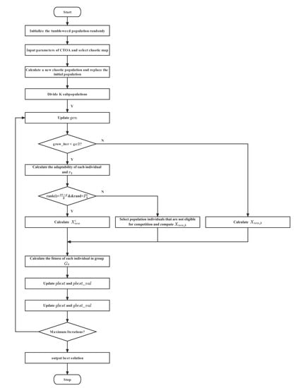
Figure 1. Flow chart of the CTOA procedure.

4. Experimental Result

In this section, we conduct experiments to determine which chaotic map is best suited for use in our proposed CTOA algorithm.

4.1. Experimental Environment and Benchmark Function

All the results presented in this section were obtained through MATLAB R2022b and Python3 simulations on a machine equipped with 11th Gen Intel(R) Core(TM) i9-11900 and 64 G RAM. Before conducting the experimental tests, we initialized the running parameters as shown in Table 3. The initial population size $pop\_size$ was set to 100 to ensure that the position distribution of individuals initialized using chaotic maps was more characteristic. The number of function runs $run\_nums$ was set to 50 to prevent random results from causing errors in the final evaluation results. To facilitate comparisons between the CTOA algorithm and the unimproved TOA algorithm, the 12 different CTOA algorithms are labeled as CPP1 to CPPE12, as shown in Table 4.

Table 3. Names of parameters and their default values.

Symbol	Preset Value
$pop\_size$	100
$run\_nums$	50
$max\_iter$	300
dim	30, 50, 100

Table 4. The meanings of algorithm symbols.

Symbol	Meaning
CTOA1	TOA + logistic map [51]
CTOA2	TOA + piecewise map [52]
CTOA3	TOA + singer map [53]
CTOA4	TOA + sine map [54]
CTOA5	TOA + Gauss map [42]
CTOA6	TOA + tent map [43]
CTOA7	TOA + Bernoulli map [55]
CTOA8	TOA + Chebyshev map [55]
CTOA9	TOA + circle map [56]
CTOA10	TOA + cubic map [57]
CTOA11	TOA + sinusoidal map [58]
CTOA12	TOA + ICMIC map [59]

The IEEE Evolutionary Computing Conference announced the appearance of the benchmark function [60] in order to conduct a comprehensive performance comparison of metaheuristic algorithms and to verify the performance of the proposed algorithm. To evaluate the performance of the proposed algorithm, we used the benchmark functions from the CEC2013 suite, which includes 28 benchmark functions separated into three categories: unimodal function, multimodal function, and composition function. Functions F1–F5 are unimodal functions, F6–F20 are multimodal functions, and F21–F28 are composite functions. The names and details of the benchmark functions are shown in Table 5, Table 6 and Table 7. Unimodal benchmark functions have a single minimum value in the search interval, which is used to test the convergence speed of CTOA. Multimodal benchmark functions have higher requirements for CTOA than unimodal functions since they have multiple local minima that can test CTOA’s ability to jump out of local optima. The composition benchmark function is a combination of the two aforementioned functions. These benchmark functions enable us to evaluate CTOA’s performance across multiple dimensions.

Table 5. Descriptive information about the unimodal benchmark function.

Unimodal Functions
Symbol	Name
F1	Sphere
F2	Rotated High Conditioned Elliptic
F3	Rotated Bent Cigar
F4	Rotated Discus
F5	Different Powers

Table 6. Descriptive information about the multimodal benchmark function.

Multimodal Functions
Symbol	Name
F6	Rotated Rosenbrock’s Function
F7	Rotated Schaffers F7 Function
F8	Rotated Ackley’s Function
F9	Rotated Weierstrass Function
F10	Rotated Griewank’s Function
F11	Rastrigin’s Function
F12	Rotated Rastrigin’s Function
F13	Non-Continuous Rotated Rastrigin’s Function
F14	Schwefel’s Function
F15	Rotated Schwefel’s Function
F16	Rotated Katsuura Function
F17	Lunacek Bi_Rastrigin Function
F18	Rotated Lunacek Bi_Rastrigin Function
F19	Expanded Griewank’s plus Rosenbrock’s Function
F20	Expanded Scaffer’s F6 Functionn

Table 7. Descriptive information about the composition benchmark function.

Composition Functions
Symbol	Name
F21	Composition Function 1 (n = 5, Rotated)
F22	Composition Function 2 (n = 3, Unrotated)
F23	Composition Function 3 (n = 3, Rotated)
F24	Composition Function 4 (n = 3, Rotated)
F25	Composition Function 5 (n = 3, Rotated)
F26	Composition Function 6 (n = 5, Rotated)
F27	Composition Function 7 (n = 5, Rotated)
F28	Composition Function 8 (n = 5, Rotated)

4.2. Experimental Result on Numerical Statistics

In the experiments, we used three criterions of algorithm performance as follows:

$$Best=min\left(hsitory\right)$$

(9)

$$Mean={\displaystyle \frac{1}{n}}\sum _{i=1}^n{x}_i$$

(10)

$$Std=\sqrt{\frac{1}{n}\sum _{i=1}^n{\left(x_i-Mean\right)}^2}$$

(11)

where $Best$ represents the algorithm’s best result in the test, $Mean$ is the average of 50 tests, and $Std$ stands for standard deviation. The historical results of the algorithm obtained after 50 runs of CEC2013 are represented by $history=[x_1,x_2,\dots ,x_{50}]$. Each algorithm’s $Best$, $Mean$, and $Std$ conditions are used to determine whether an experiment is good or bad. The $Best$ reflects the algorithm’s limit, the $Mean$ reflects the algorithm’s accuracy, and the $Std$ reflects the algorithm’s stability. To demonstrate the performance and robustness of CTOA in different dimensions, we run CTOA, presented in Table 4, at 30D, 50D, and 100D, and record the experimental data in these dimensions.

In addition, in order to visually demonstrate the improvement of the TOA by the initialization of the chaotic map, the experimental results of TOA in these three dimensions are also counted in the table. Table 8, Table 9, Table 10 and Table 11 record the results of the algorithms in Table 4 running in 30D, Table 12, Table 13, Table 14 and Table 15 record the results of running in 50D, and Table 16, Table 17, Table 18 and Table 19 record the results of running in 100D. Note that the experiments’ best results have been highlighted in bold.

Table 8. Experimental results running on F1–F8 in 30D.

F1	Best	Mean	Std	F2	Best	Mean	Std
TOA	1.430592755	4.641731	2.480966	TOA	11,473,867.54	34,462,604.66	14,601,957
CTOA1	1.356563975	4.821175	2.266016	CTOA1	13,145,120.42	40,300,671.68	14,502,168
CTOA2	2.172104923	5.053772	2.030593	CTOA2	15,487,711.82	37,557,028.96	14,565,769
CTOA3	2.172104923	4.657546	2.175062	CTOA3	15,487,711.82	38,253,389.61	16,509,389
CTOA4	1.546960909	4.428686	2.417921	CTOA4	6,523,850.195	35,940,710.69	17,492,089
CTOA5	1.837306316	4.976843	2.274063	CTOA5	9,265,487.406	31,802,326.54	13,703,389
CTOA6	1.224058288	4.485701	1.835378	CTOA6	16,328,752.4	34,694,526.92	13,762,606
CTOA7	1.123754048	4.805862	2.795162	CTOA7	6,257,637.872	36,435,707.09	16,837,924
CTOA8	1.725739828	5.240968	2.542584	CTOA8	12,313,227	38,175,833.98	15,679,630
CTOA9	0.888030114	3.973734	1.635657	CTOA9	11,532,968.2	31,333,746.02	12,639,456
CTOA10	1.861330464	4.274323	1.990519	CTOA10	14,008,982.47	34,391,752.87	15,362,061
CTOA11	1.653179427	4.358769	1.778436	CTOA11	10,443,066.7	38,167,456.83	17,836,779
CTOA12	1.173376114	4.510318	2.069676	CTOA12	5,277,183.485	34,464,024.71	11,813,327
F3	Best	Mean	Std	F4	Best	Mean	Std
TOA	$\mathbf{1}.\mathbf{45}\times {\mathbf{10}}^{\mathbf{8}}$	$7.42\times {10}^9$	$8.12\times {10}^9$	TOA	35,475.60207	73,183.97463	18,858.371
CTOA1	$1.19\times {10}^9$	$9.64\times {10}^9$	$8.31\times {10}^9$	CTOA1	38,800.81737	77,107.95584	19,576.841
CTOA2	$8.47\times {10}^8$	$8.50\times {10}^9$	$9.10\times {10}^9$	CTOA2	21,634.29326	70,535.35488	22,998.472
CTOA3	$8.47\times {10}^8$	$1.08\times {10}^{10}$	$1.00\times {10}^{10}$	CTOA3	21,634.29326	71,190.58643	18,545.374
CTOA4	$3.18\times {10}^8$	$8.24\times {10}^9$	$8.33\times {10}^9$	CTOA4	33,931.41384	77,808.57394	18,384.651
CTOA5	$2.52\times {10}^9$	$8.78\times {10}^9$	$7.68\times {10}^9$	CTOA5	37,761.57951	70,942.00626	19,069.629
CTOA6	$1.78\times {10}^8$	$8.97\times {10}^9$	$9.86\times {10}^9$	CTOA6	28,886.6629	73,846.69415	23,766.912
CTOA7	$2.36\times {10}^8$	$\mathbf{7}.\mathbf{19}\times {\mathbf{10}}^{\mathbf{9}}$	$6.68\times {10}^9$	CTOA7	39,749.64181	74,221.0471	19,434.414
CTOA8	$7.81\times {10}^8$	$7.47\times {10}^9$	$\mathbf{5}.\mathbf{77}\times {\mathbf{10}}^{\mathbf{9}}$	CTOA8	29,124.27816	72,806.70522	20,911.395
CTOA9	$7.06\times {10}^8$	$7.28\times {10}^9$	$6.09\times {10}^9$	CTOA9	27,021.25272	56,943.74888	16,380.353
CTOA10	$6.57\times {10}^8$	$1.04\times {10}^{10}$	$8.99\times {10}^9$	CTOA10	38,838.69185	75,038.99139	21,096.963
CTOA11	$6.03\times {10}^8$	$9.00\times {10}^9$	$6.77\times {10}^9$	CTOA11	31,035.217	71,643.12255	19,231.639
CTOA12	$9.26\times {10}^8$	$8.77\times {10}^9$	$9.02\times {10}^9$	CTOA12	33,858.73636	72,004.99112	20,686.456
F5	Best	Mean	Std	F6	Best	Mean	Std
CTOA	6.641295	43.86907	33.70866	CTOA	23.26008	75.81029	30.20365
CTOA1	7.240699	50.98158	43.35798	CTOA1	29.37788	82.79009	30.15121
CTOA2	7.448614	45.8111	33.21403	CTOA2	23.13454	86.01479	37.35468
CTOA3	7.448614	47.1076	39.57283	CTOA3	23.13454	84.56738	27.91947
CTOA4	7.229537	54.54368	36.60177	CTOA4	21.10389	75.55618	30.1907
CTOA5	8.671002	55.66441	42.5454	CTOA5	24.53502	85.32412	35.90527
CTOA6	8.313796	53.25556	38.6086	CTOA6	26.59667	82.49312	30.82995
CTOA7	5.533057	42.19865	32.58633	CTOA7	22.55549	80.02851	32.46554
CTOA8	4.249546	53.05737	40.30658	CTOA8	30.61643	83.21242	32.14927
CTOA9	7.34457	42.41004	35.593	CTOA9	20.84706	84.79518	33.58295
CTOA10	4.87272	49.02898	37.55706	CTOA10	17.78542	73.81029	27.75425
CTOA11	6.820977	51.17952	35.98522	CTOA11	21.03715	78.78057	28.70238
CTOA12	7.154989	47.78411	38.08524	CTOA12	23.17294	76.62523	28.75425
F7	Best	Mean	Std	F8	Best	Mean	Std
TOA	69.42176	172.0952	49.69714	TOA	20.87601	21.05851	0.057536
CTOA1	74.3429	164.016	40.48377	CTOA1	20.98392	21.08069	0.039275
CTOA2	52.15573	169.4007	50.64785	CTOA2	20.97782	21.08017	0.047848
CTOA3	52.15573	169.0283	59.16052	CTOA3	20.97782	21.05609	0.056827
CTOA4	57.95494	164.9569	48.58436	CTOA4	20.84488	21.05512	0.066816
CTOA5	65.19426	146.1801	45.96157	CTOA5	20.92916	21.0642	0.053411
CTOA6	62.15799	162.4576	53.75279	CTOA6	20.88531	21.06649	0.056811
CTOA7	69.76826	157.5119	46.9178	CTOA7	20.93686	21.06587	0.048774
CTOA8	64.50866	172.4547	57.10363	CTOA8	20.93791	21.05956	0.057127
CTOA9	62.14251	143.9033	50.76479	CTOA9	20.78702	21.06498	0.061698
CTOA10	65.2948	167.2855	58.53906	CTOA10	20.84606	21.05344	0.063907
CTOA11	74.50113	159.8454	56.96794	CTOA11	20.85003	21.04871	0.058645
TOA12	49.67303	150.4142	55.90276	TOA12	20.92519	21.06103	0.059276

Table 9. Experimental results running on F9–F16 in 30D.

F9	Best	Mean	Std	F10	Best	Mean	Std
TOA	19.47632	30.36987	3.079732	TOA	26.22931	82.35212	26.96656
CTOA1	23.6859	30.08422	2.410925	CTOA1	36.85686	87.32382	29.07486
CTOA2	18.96248	30.19011	3.150221	CTOA2	36.19492	84.57543	27.17525
CTOA3	18.96248	30.13138	3.067458	CTOA3	36.19492	87.67734	30.95377
CTOA4	22.84056	30.6682	2.287681	CTOA4	35.7127	87.19001	32.80739
CTOA5	20.81174	29.67086	2.776753	CTOA5	27.46838	81.2549	30.55649
CTOA6	21.76101	28.90034	2.665711	CTOA6	38.87631	86.58836	29.73541
CTOA7	25.24309	30.58017	2.705951	CTOA7	33.20027	79.27575	28.61971
CTOA8	18.28933	30.58495	2.794156	CTOA8	26.14432	83.678	34.17651
CTOA9	18.94317	29.24522	2.631635	CTOA9	23.38867	73.87533	25.42127
CTOA10	23.18855	29.95208	2.470231	CTOA10	21.04443	81.61116	29.87273
CTOA11	19.05223	29.73277	3.148697	CTOA11	17.86598	92.65487	39.57157
CTOA12	20.69468	29.59942	3.377856	CTOA12	26.10178	84.09473	23.51075
F11	Best	Mean	Std	F12	Best	Mean	Std
TOA	83.99478	184.951	68.01735	TOA	91.25174	211.4995	55.09605
CTOA1	52.58211	189.8489	85.23317	CTOA1	88.95786	198.6493	76.84806
CTOA2	78.39617	184.2122	66.12921	CTOA2	124.0647	219.8842	53.86497
CTOA3	78.39617	160.9085	80.6409	CTOA3	124.0647	221.2579	85.30896
CTOA4	68.34443	172.4444	82.54131	CTOA4	94.24765	218.445	77.4122
CTOA5	93.28622	188.8487	70.54447	CTOA5	82.40928	222.4609	52.09472
CTOA6	61.4155	181.6452	71.13292	CTOA6	122.7949	202.9098	40.47806
CTOA7	97.55595	191.7591	66.90959	CTOA7	98.03852	234.5548	84.43587
CTOA8	60.38598	184.2558	83.72744	CTOA8	69.61156	215.1982	75.49402
CTOA9	84.5647	149.2546	43.80927	CTOA9	96.40827	199.086	50.27889
CTOA10	71.89555	181.625	102.8933	CTOA10	64.21004	213.7707	69.99723
CTOA11	59.81794	183.3453	91.25827	CTOA11	85.6472	217.8867	71.39717
CTOA12	53.47842	164.3092	66.89424	CTOA12	61.59151	204.1543	57.38563
F13	Best	Mean	Std	F14	Best	Mean	Std
TOA	158.7791	230.7484	34.13018	TOA	370.135	4981.427	1395.315
CTOA1	75.41791	237.9464	49.72082	CTOA1	2590.528	5234.083	1,164.151
CTOA2	152.7115	236.5774	36.13152	CTOA2	2229.513	5326.335	1309.164
CTOA3	152.7115	223.2597	31.3048	CTOA3	2229.513	4330.862	1383.245
CTOA4	127.9629	227.1254	33.32703	CTOA4	2113.416	4909.046	1347.483
CTOA5	153.3039	245.4698	38.51728	CTOA5	2181.083	5726.357	1279.679
CTOA6	131.3499	239.4234	45.30911	CTOA6	1049.555	5145.848	1378.694
CTOA7	141.2002	238.685	40.63646	CTOA7	2658.65	5166.621	1272.206
CTOA8	159.901	238.103	41.95559	CTOA8	2192.565	5007.671	1432.373
CTOA9	116.513	230.5702	37.28941	CTOA9	2256.723	5596.839	1221.914
CTOA10	147.9437	228.7623	39.40842	CTOA10	1657.245	4579.721	1460.737
CTOA11	140.8689	230.2052	37.49626	CTOA11	2925.443	5502.232	1255.026
CTOA12	143.2574	229.6021	35.7941	CTOA12	2371.384	5041.32	1423.715
F15	Best	Mean	Std	F16	Best	Mean	Std
TOA	5,641.266	6,704.208	423.7036	TOA	2.364631	3.197233	0.348217
CTOA1	5,492.424	6,700.285	536.451	CTOA1	1.804553	3.179833	0.421851
CTOA2	5844.424	6783.61	352.2824	CTOA2	2.431884	3.230702	0.35488
CTOA3	5844.424	6756.636	379.1114	CTOA3	2.431884	3.243784	0.381423
CTOA4	5853.198	6726.53	402.9906	CTOA4	2.043303	3.205199	0.449456
CTOA5	5675.896	6713.259	490.0271	CTOA5	2.403875	3.181841	0.379426
CTOA6	5866.364	6686.728	340.3926	CTOA6	2.140888	3.256858	0.364961
CTOA7	5,651.658	6727.874	415.1401	CTOA7	2.085766	3.224259	0.427801
CTOA8	5047.775	6879.885	503.5179	CTOA8	1.689464	3.225949	0.389588
CTOA9	5809.945	6596.72	407.5732	CTOA9	2.176599	3.208446	0.396451
CTOA10	5411.916	6665.79	456.1787	CTOA10	2.458289	3.304063	0.319186
CTOA11	3720.667	6728.399	612.8474	CTOA11	2.535856	3.225695	0.371798
CTOA12	5348.347	6662.602	518.1656	CTOA12	2.28681	3.287651	0.369558

Table 10. Experimental results running on F17–F24 in 30D.

F17	Best	Mean	Std	F18	Best	Mean	Std
TOA	191.1994	255.4997	25.7751	TOA	235.7625	276.4613	21.39819
CTOA1	187.7217	253.7246	33.70481	CTOA1	221.4716	270.5805	21.67858
CTOA2	169.3405	254.9586	39.27158	CTOA2	233.0861	278.8428	21.98578
CTOA3	169.3405	244.7709	34.22477	CTOA3	233.0861	270.2849	24.28905
CTOA4	186.7281	256.2904	23.41873	CTOA4	206.8143	274.8773	29.38987
CTOA5	192.9143	259.269	31.58694	CTOA5	203.0203	278.0344	22.9301
CTOA6	166.0398	256.9565	27.88832	CTOA6	190.8338	272.6024	28.12443
CTOA7	132.5832	251.8977	37.64356	CTOA7	210.1343	270.0525	23.33517
CTOA8	146.7767	250.2936	31.07202	CTOA8	225.6414	273.9212	26.46477
CTOA9	206.8276	258.6434	23.38194	CTOA9	232.0053	278.0042	19.69428
CTOA10	173.7475	244.1345	27.17231	CTOA10	219.1796	276.0129	22.75225
CTOA11	182.298	244.3409	24.40894	CTOA11	198.8819	271.6275	27.12828
CTOA12	169.2201	248.6996	39.51309	CTOA12	191.3392	268.9461	23.80379
F19	Best	Mean	Std	F20	Best	Mean	Std
TOA	8.823527	16.3698	2.460191	TOA	12.11205	13.77631	0.857837
CTOA1	9.968513	15.65698	2.717404	CTOA1	12.02135	14.121	0.944627
CTOA2	9.507782	16.17751	2.687117	CTOA2	12.1312	13.7874	0.966827
CTOA3	9.507782	15.98989	2.328031	CTOA3	12.1312	14.70137	0.623059
CTOA4	7.683536	15.54814	2.957507	CTOA4	12.10369	13.90993	1.000377
CTOA5	9.423743	16.86574	3.039682	CTOA5	12.26715	13.8474	0.922043
CTOA6	9.344505	16.18553	2.596153	CTOA6	12.45917	13.95253	0.9019
CTOA7	10.22913	16.58573	2.306279	CTOA7	12.24273	13.85383	0.870465
CTOA8	10.33814	17.476	2.959561	CTOA8	12.19564	14.27576	0.937514
CTOA9	7.663299	16.29275	2.838714	CTOA9	12.11917	13.35693	0.829536
CTOA10	9.866316	16.15057	2.232672	CTOA10	12.03096	14.42613	0.862933
CTOA11	9.879782	16.27021	2.127274	CTOA11	12.64206	13.82569	0.896084
CTOA12	10.8117	16.41916	2.60959	CTOA12	12.29212	14.28751	0.881478
F21	Best	Mean	Std	F22	Best	Mean	Std
TOA	221.5507	320.7292	77.89905	TOA	2492.254	5457.696	1573.757
CTOA1	224.3926	338.6655	67.01389	CTOA1	2492.687	5158.906	1359.081
CTOA2	228.3312	345.0221	70.27384	CTOA2	2447.092	5314.307	1589.62
CTOA3	228.3312	390.3265	75.39317	CTOA3	2447.092	4512.892	1469.588
CTOA4	223.1676	317.3854	59.91028	CTOA4	2290.699	5077.663	1546.049
CTOA5	229.7998	345.6994	63.40178	CTOA5	2525.532	5355.718	1510.444
CTOA6	221.131	327.843	70.1972	CTOA6	2145.753	5356.283	1524.727
CTOA7	226.7677	330.3168	80.79807	CTOA7	2389.541	4995.464	1485.753
CTOA8	239.3515	372.9876	63.48176	CTOA8	2807.814	5130.634	1500.005
CTOA9	151.2828	340.4276	85.9303	CTOA9	1767.661	5502.564	1575.352
CTOA10	231.9426	366.2842	66.6869	CTOA10	2085.168	4617.966	1366.792
CTOA11	144.8216	326.723	64.16248	CTOA11	1726.552	5435.613	1503.185
CTOA12	227.8882	355.7093	71.40169	CTOA12	2573.423	5136.566	1429.554
F23	Best	Mean	Std	F24	Best	Mean	Std
TOA	5745.163	6987.26	593.466	TOA	258.6309	280.5159	9.064905
CTOA1	4752.849	7019.605	578.4228	CTOA1	255.5681	281.4412	9.676793
CTOA2	5733.22	6849.891	509.0746	CTOA2	261.4231	278.0223	9.020633
CTOA3	5733.22	7083.667	634.6992	CTOA3	261.4231	280.7545	10.68703
CTOA4	3445.902	7021.244	746.902	CTOA4	257.7895	280.7787	8.778902
CTOA5	4346.894	6910.548	693.303	CTOA5	261.2685	281.4815	9.309686
CTOA6	5486.644	7006.287	534.5366	CTOA6	254.2371	280.8182	8.424572
CTOA7	4405.119	6904.682	596.9329	CTOA7	262.5834	282.3798	10.07625
CTOA8	5926.2	7073.831	425.523	CTOA8	259.4419	281.1743	8.740838
CTOA9	5569.926	6909.94	562.6803	CTOA9	258.8804	278.1883	9.733462
CTOA10	5306.714	7035.998	605.8532	CTOA10	262.2337	280.2527	8.71317
CTOA11	4864.535	6960.24	550.5438	CTOA11	253.8493	281.7362	9.510098
CTOA12	5198.507	7067.133	589.5727	CTOA12	260.3661	281.6952	8.436596

Table 11. Experimental results running on F25–F28 in 30D.

F25	Best	Mean	Std	F26	Best	Mean	Std
TOA	273.0118	287.2744	7.030919	TOA	200.6034	354.0326	59.18926
CTOA1	268.2402	289.4821	9.246821	CTOA1	201.2018	363.4794	39.86875
CTOA2	263.9079	289.2079	10.62954	CTOA2	200.9928	348.8948	61.49499
CTOA3	263.9079	290.1613	8.282695	CTOA3	200.9928	361.3564	45.71191
CTOA4	271.37	290.9549	7.802634	CTOA4	200.7299	336.1142	71.6734
CTOA5	268.3196	288.309	9.57809	CTOA5	200.8854	323.861	78.67613
CTOA6	272.7219	289.6455	8.917811	CTOA6	201.0962	342.5849	67.12981
CTOA7	270.4478	287.1193	8.792928	CTOA7	200.9794	324.4437	79.27322
CTOA8	261.0774	286.462	9.807126	CTOA8	200.9593	345.9068	64.36845
CTOA9	274.7382	288.257	7.665817	CTOA9	200.6327	300.2476	84.35678
CTOA10	261.1317	290.5119	9.435829	CTOA10	201.4667	351.6566	58.12046
CTOA11	271.1873	288.9337	8.883081	CTOA11	201.7781	356.0028	54.79191
CTOA12	271.8485	288.5178	10.21368	CTOA12	200.4804	347.4318	65.64149
F27	Best	Mean	Std	F28	Best	Mean	Std
TOA	871.0711	1067.818	74.45373	TOA	365.7219	540.8311	331.938
CTOA1	889.2358	1074.299	94.31119	CTOA1	382.1719	471.1867	180.0546
CTOA2	817.416	1060.77	96.08947	CTOA2	376.2239	487.178	229.1578
CTOA3	817.416	1050.325	91.33763	CTOA3	376.2239	798.954	534.3881
CTOA4	838.4956	1062.829	87.493	CTOA4	199.8576	539.2765	344.8095
CTOA5	848.5246	1060.985	97.76764	CTOA5	365.4524	465.2611	176.5598
CTOA6	913.9902	1089.694	74.84623	CTOA6	355.3892	467.7049	228.928
CTOA7	925.1872	1065.879	66.1941	CTOA7	362.0028	474.912	186.4551
CTOA8	787.3533	1051.827	95.20461	CTOA8	364.9942	716.584	493.1192
CTOA9	802.638	1035.468	94.99268	CTOA9	173.6509	569.9431	488.5328
CTOA10	834.2885	1059.74	71.8523	CTOA10	372.0484	613.7077	416.3061
CTOA11	805.3148	1068.097	106.2754	CTOA11	358.9237	497.9177	274.4063
CTOA12	867.2102	1055.543	79.59421	CTOA12	368.3432	595.7947	412.9015

Table 12. Experimental results running on F1–F8 in 50D.

F1	Best	Mean	Std	F2	Best	Mean	Std
TOA	47.93336	95.11479	28.91364	TOA	41,084,347.19	99,934,056.86	34,099,495.64
CTOA1	34.9045	94.45528	32.11812	CTOA1	42,291,631.58	118,694,884.5	53,959,926.18
CTOA2	47.43622	92.69795	28.15622	CTOA2	31,492,325.05	98,563,069.62	35,177,164.77
CTOA3	47.43622	103.5596	39.20834	CTOA3	31,492,325.05	85,470,333.09	32,099,117.51
CTOA4	40.57444	93.33722	32.53762	CTOA4	52,376,457.15	105,263,004.5	34,615,169.58
CTOA5	36.31797	89.70178	29.7691	CTOA5	26,539,157.33	96,278,699.58	33,363,342.28
CTOA6	35.32903	79.83578	25.19787	CTOA6	36,551,438.45	102,373,582.7	34,779,463.74
CTOA7	32.20098	93.57819	25.68838	CTOA7	34,362,723.34	108,909,903.4	37,210,665.71
CTOA8	50.29742	97.94228	30.97021	CTOA8	32,613,735.73	99,479,035.01	38,945,154.25
CTOA9	27.19391	82.61719	25.84005	CTOA9	34,431,771.11	91,858,862.99	33,124,113.91
CTOA10	37.86909	96.3431	31.09465	CTOA10	49,408,842.68	95,765,681.89	32,726,320.96
CTOA11	30.1694	93.62948	35.38649	CTOA11	39,317,874.31	114,310,927.2	36,819,144.93
CTOA12	36.27405	102.8991	36.37749	CTOA12	30,172,910.2	93,505,723.77	33,490,234.19
F3	Best	Mean	Std	F4	Best	Mean	Std
TOA	$1.10\times {10}^{10}$	$5.63\times {10}^{10}$	$3.03\times {10}^{10}$	TOA	84,777.91	131,966.9	26,642.19
CTOA1	$1.12\times {10}^{10}$	$6.37\times {10}^{10}$	$3.93\times {10}^{10}$	CTOA1	74,253.14	145,774.3	28,144.54
CTOA2	$1.57\times {10}^{10}$	$5.73\times {10}^{10}$	$2.62\times {10}^{10}$	CTOA2	80,255.77	13,0762	26,760.39
CTOA3	$1.57\times {10}^{10}$	$6.16\times {10}^{10}$	$3.27\times {10}^{10}$	CTOA3	80,255.77	144,831.5	22,728.45
CTOA4	$1.33\times {10}^{10}$	$5.87\times {10}^{10}$	$3.51\times {10}^{10}$	CTOA4	84,808.8	138,823.9	25,367.29
CTOA5	$9.64\times {10}^9$	$5.71\times {10}^{10}$	$3.01\times {10}^{10}$	CTOA5	87,829.8	137,195.7	30,456.33
CTOA6	$1.49\times {10}^{10}$	$5.44\times {10}^{10}$	$3.16\times {10}^{10}$	CTOA6	84,565.71	137,910.8	29,164.56
CTOA7	$8.16\times {10}^{09}$	$5.63\times {10}^{10}$	$2.83\times {10}^{10}$	CTOA7	72,567.08	132,362.6	24,210.28
CTOA8	$1.23\times {10}^{10}$	$5.99\times {10}^{10}$	$3.42\times {10}^{10}$	CTOA8	81,541.39	144628.5	28,494.84
CTOA9	$1.14\times {10}^{10}$	$\mathbf{4}.\mathbf{80}\times {\mathbf{10}}^{\mathbf{10}}$	$\mathbf{2}.\mathbf{59}\times {\mathbf{10}}^{\mathbf{10}}$	CTOA9	44,350.31	114,722	29,349.97
CTOA10	$1.60\times {10}^{10}$	$6.35\times {10}^{10}$	$3.68\times {10}^{10}$	CTOA10	77,112.54	149,794.9	30,334.24
CTOA11	$\mathbf{4}.\mathbf{39}\times {\mathbf{10}}^{\mathbf{9}}$	$6.08\times {10}^{10}$	$2.97\times {10}^{10}$	CTOA11	91,002.13	145,502.5	29,185.3
CTOA12	$1.92\times {10}^{10}$	$6.19\times {10}^{10}$	$2.96\times {10}^{10}$	CTOA12	94,817.95	141,163.3	25,052.11
F5	Best	Mean	Std	F6	Best	Mean	Std
TOA	99.03806	250.2416	56.99093	TOA	59.3082	138.5892	62.55081
CTOA1	164.8707	258.2605	48.80763	CTOA1	53.21279	138.1261	72.29992
CTOA2	101.2389	234.1355	53.17557	CTOA2	54.99738	134.8758	66.50206
CTOA3	101.2389	240.0413	43.43521	CTOA3	54.99738	125.7091	52.0445
CTOA4	153.2694	244.6653	55.86586	CTOA4	53.897	149.335	81.68212
CTOA5	145.2499	250.2859	49.50397	CTOA5	60.98863	148.4365	62.64033
CTOA6	115.056	237.4776	50.40263	CTOA6	60.54749	176.6171	99.92527
CTOA7	141.4791	244.1527	56.49436	CTOA7	60.2818	145.1284	71.4382
CTOA8	146.7977	247.3407	46.18892	CTOA8	54.10226	121.4684	68.49735
CTOA9	93.25496	204.8941	49.13547	CTOA9	55.34641	184.4958	75.70716
CTOA10	153.3158	246.8471	51.27477	CTOA10	58.27578	134.2529	62.65023
CTOA11	140.5322	245.5632	50.01144	CTOA11	54.10269	151.2276	83.53149
CTOA12	111.2616	247.5164	53.58613	CTOA12	51.66511	140.3907	80.9856
F7	Best	Mean	Std	F8	Best	Mean	Std
TOA	145.07	220.9826	37.64836	TOA	21.13861	21.23259	0.037738
CTOA1	140.9811	225.785	35.92001	CTOA1	21.16599	21.24026	0.035016
CTOA2	149.2201	225.4816	41.60381	CTOA2	21.13512	21.2329	0.042212
CTOA3	149.2201	214.8705	40.45722	CTOA3	21.13512	21.23274	0.032241
CTOA4	144.899	229.977	47.38471	CTOA4	21.12333	21.23475	0.037583
CTOA5	127.4234	217.5407	41.26043	CTOA5	21.08971	21.23532	0.039473
CTOA6	141.953	222.519	44.4323	CTOA6	21.06378	21.23042	0.047104
CTOA7	146.5261	227.5686	42.63456	CTOA7	21.11766	21.23728	0.042119
CTOA8	134.3188	224.0099	44.08832	CTOA8	21.10592	21.22182	0.045104
CTOA9	153.0399	197.5499	32.38021	CTOA9	21.13364	21.22656	0.041457
CTOA10	152.5624	219.9995	38.21989	CTOA10	21.11138	21.22743	0.039115
CTOA11	156.7244	225.0154	37.59788	CTOA11	21.11089	21.23803	0.039791
CTOA12	156.3481	230.7091	35.6285	CTOA12	21.09986	21.22616	0.031283

Table 13. Experimental results running on F9–F16 in 50D.

F9	Best	Mean	Std	F10	Best	Mean	Std
TOA	51.45157	59.57449	3.825761	TOA	201.8683	512.4316	152.7787
CTOA1	41.64605	59.7855	4.621395	CTOA1	223.5617	526.1229	177.7425
CTOA2	45.23146	59.54556	4.797162	CTOA2	222.9015	512.9366	159.1014
CTOA3	45.23146	59.78384	4.70706	CTOA3	222.9015	551.9805	159.475
CTOA4	49.61566	60.20404	3.856908	CTOA4	222.8496	545.2075	172.0383
CTOA5	47.34207	60.13432	3.732362	CTOA5	294.1571	522.3137	137.4475
CTOA6	49.42004	59.63004	3.83985	CTOA6	285.4589	524.9346	127.5325
CTOA7	49.59141	60.36408	4.014266	CTOA7	264.6706	507.5844	172.0069
CTOA8	51.06752	59.93045	4.031302	CTOA8	254.771	531.7375	155.2429
CTOA9	44.56648	59.30775	4.735694	CTOA9	180.2026	392.0369	133.6758
CTOA10	46.65123	59.13262	4.279494	CTOA10	279.9391	553.1651	151.1298
CTOA11	45.9285	59.80617	4.059403	CTOA11	155.7072	498.1528	185.5661
CTOA12	43.07219	59.4426	4.961187	CTOA12	281.5639	528.0257	148.9916
F11	Best	Mean	Std	F12	Best	Mean	Std
TOA	202.4885	425.8454	147.228	TOA	333.6475	564.8086	123.9431
CTOA1	193.1398	371.4938	158.5099	CTOA1	317.1222	525.0204	157.263
CTOA2	207.4459	428.3898	136.4808	CTOA2	279.2988	543.1633	97.22959
CTOA3	207.4459	314.6289	115.309	CTOA3	279.2988	465.4323	95.89378
CTOA4	208.9741	399.9909	169.4385	CTOA4	310.2108	535.3492	126.2113
CTOA5	242.8699	443.0413	154.8247	CTOA5	338.1129	555.84	137.8974
CTOA6	187.5576	409.1792	143.4178	CTOA6	287.6132	539.7874	119.8936
CTOA7	208.0959	410.4099	155.6475	CTOA7	272.1977	543.798	120.2503
CTOA8	177.2906	327.4294	131.058	CTOA8	257.715	508.1558	106.0107
CTOA9	181.8226	317.4527	63.29728	CTOA9	237.0802	495.5171	98.54498
CTOA10	180.6447	320.9195	115.4608	CTOA10	274.0202	528.3227	129.1037
CTOA11	162.8652	406.3214	200.7118	CTOA11	294.8029	519.6554	141.327
CTOA12	169.1461	356.275	145.6271	CTOA12	270.8147	493.449	99.98
F13	Best	Mean	Std	F14	Best	Mean	Std
TOA	436.0461	567.7784	64.67605	TOA	6308.859	10,709.21	1976.852
CTOA1	381.628	545.4609	70.37456	CTOA1	6592.325	10,332.31	2182.163
CTOA2	428.9403	554.1061	57.51002	CTOA2	5669.642	10,351.63	2351.777
CTOA3	428.9403	546.2776	73.60519	CTOA3	5669.642	9754.155	2129.36
CTOA4	399.2063	559.4091	71.64018	CTOA4	4981.227	10,460.02	2225.211
CTOA5	441.7775	557.3963	52.42537	CTOA5	5656.661	10,577.26	2429.533
CTOA6	429.1183	553.5367	57.40065	CTOA6	5775.554	10,267.94	2257.291
CTOA7	409.0477	554.6424	72.04844	CTOA7	5269.51	10,462.15	2136.355
CTOA8	439.4703	544.0158	55.05047	CTOA8	5604.988	9649.748	2224.881
CTOA9	408.3318	535.0959	61.93543	CTOA9	5947.821	11344.19	1745.503
CTOA10	421.2888	541.2879	67.65827	CTOA10	5614.678	9714.602	2152.191
CTOA11	442.0623	544.7147	59.228	CTOA11	5914.19	10,617.1	2068.622
CTOA12	389.8412	555.7978	57.31587	CTOA12	4792.576	10,080.58	2270.388
F15	Best	Mean	Std	F16	Best	Mean	Std
TOA	11,830.1	13,501.17	581.1357	TOA	3.313326	4.228536	0.365848
CTOA1	12,583.1	13,601.45	505.4042	CTOA1	3.294737	4.306704	0.427229
CTOA2	11,278.57	13,293.68	681.5553	CTOA2	3.506279	4.215137	0.374083
CTOA3	11,278.57	13,496.54	654.1637	CTOA3	3.506279	4.230933	0.45455
CTOA4	12,209.93	13,507.25	588.4897	CTOA4	3.074484	4.255058	0.371441
CTOA5	11,556.41	13,506.37	615.3785	CTOA5	3.055281	4.345794	0.394799
CTOA6	12,088.27	13,549.69	589.0859	CTOA6	3.07	4.268821	0.380532
CTOA7	11,545	13,371.58	633.3576	CTOA7	3.379483	4.277709	0.374405
CTOA8	11,994.78	13,360.58	539.282	CTOA8	2.947859	4.213767	0.445558
CTOA9	11,274.89	13,299	723.3836	CTOA9	3.460457	4.229747	0.401068
CTOA10	11,426.02	13,421.82	751.7903	CTOA10	3.134472	4.250979	0.37598
CTOA11	10,332.05	13,328.76	728.8364	CTOA11	3.243943	4.160206	0.399226
CTOA12	11,445	13,369.95	659.8026	CTOA12	3.247016	4.296071	0.41248

Table 14. Experimental results running on F17–F24 in 50D.

F17	Best	Mean	Std	F18	Best	Mean	Std
TOA	480.3804	573.0563	41.62288	TOA	497.8693	612.4716	44.17009
CTOA1	418.0995	564.0892	55.55246	CTOA1	476.1289	594.5204	46.58823
CTOA2	455.7556	576.9159	49.14111	CTOA2	518.5532	612.6539	45.57987
CTOA3	455.7556	579.3593	65.88425	CTOA3	518.5532	614.307	39.44276
CTOA4	455.9066	565.2084	50.36234	CTOA4	496.0631	613.414	53.27447
CTOA5	392.9427	574.7266	60.17637	CTOA5	514.5905	603.9153	41.95238
CTOA6	442.965	580.516	62.5196	CTOA6	498.523	602.945	48.8578
CTOA7	441.4105	564.3685	56.01363	CTOA7	515.0777	608.997	49.55836
CTOA8	470.8075	578.2508	53.33804	CTOA8	517.8969	604.3338	42.79912
CTOA9	417.0029	574.8594	66.85133	CTOA9	490.2215	604.0954	48.37033
CTOA10	478.4479	580.2806	52.12733	CTOA10	525.3301	609.8586	46.59068
CTOA11	505.5884	589.0939	51.13322	CTOA11	490.6751	611.8601	52.8092
CTOA12	430.3107	573.8725	55.43454	CTOA12	545.5884	613.9124	41.83909
F19	Best	Mean	Std	F20	Best	Mean	Std
TOA	30.18974	44.00778	8.1584	TOA	21.96708	23.69333	0.665196
CTOA1	24.03189	41.10034	7.445552	CTOA1	22.70291	23.72985	0.711473
CTOA2	28.46762	44.44436	7.782507	CTOA2	22.38762	23.57221	0.725435
CTOA3	28.46762	45.28228	6.061791	CTOA3	22.38762	24.70893	0.496085
CTOA4	26.50224	43.00992	7.174469	CTOA4	22.33911	23.73272	0.680642
CTOA5	33.58467	43.55086	5.655209	CTOA5	22.34395	23.64211	0.728987
CTOA6	30.4168	43.1112	6.12804	CTOA6	22.33165	23.59186	0.588184
CTOA7	33.46082	43.95716	5.581733	CTOA7	22.01768	23.78482	0.824475
CTOA8	34.4927	45.45706	7.094966	CTOA8	22.35792	24.26676	0.777374
CTOA9	28.67901	44.72493	6.887457	CTOA9	22.16108	23.33785	0.591785
CTOA10	30.86927	42.50062	7.678287	CTOA10	22.71713	24.21457	0.70456
CTOA11	30.87846	42.26517	4.838191	CTOA11	22.58374	24.04589	0.730946
CTOA12	30.47774	43.94989	7.037634	CTOA12	22.38252	24.08283	0.690602
F21	Best	Mean	Std	F22	Best	Mean	Std
TOA	327.7914	890.582	353.0427	TOA	4,905.229	10,591.85	2416.849
CTOA1	345.2566	971.2165	346.4438	CTOA1	6211.514	10,631.96	2632.582
CTOA2	352.0457	966.1944	345.9517	CTOA2	6501.444	11,174.2	2270.215
CTOA3	352.0457	830.6496	385.3888	CTOA3	6501.444	10,033.79	2348.71
CTOA4	363.9412	1032.962	317.326	CTOA4	6121.501	10,465.86	2039.65
CTOA5	369.2878	996.6293	330.4367	CTOA5	6947.346	11,076.81	2143.838
CTOA6	350.811	926.88	352.874	CTOA6	6170.2	11,002.7	2324.04
CTOA7	319.4219	864.8827	380.6891	CTOA7	6678.996	10,567.01	2363.718
CTOA8	348.5268	868.3168	397.7172	CTOA8	6427.289	10,406.05	2287.282
CTOA9	328.2194	984.5259	299.4723	CTOA9	6429.718	11,047.88	2078.408
CTOA10	322.234	875.9508	396.4327	CTOA10	5588.184	10,258.95	2431.827
CTOA11	349.8816	1015.039	330.551	CTOA11	6830.04	10,983.99	2195.861
CTOA12	342.6955	848.8454	390.3914	CTOA12	7121.26	10,498.44	2159.198
F25	Best	Mean	Std	F26	Best	Mean	Std
TOA	341.3034	378.1281	14.44046	TOA	205.5451	442.7682	35.61185
CTOA1	351.4246	377.3641	13.37185	CTOA1	415.301	447.7863	11.94769
CTOA2	334.7624	379.2971	17.34367	CTOA2	213.0823	443.4381	34.24711
CTOA3	334.7624	378.0456	15.14113	CTOA3	213.0823	448.0654	13.32695
CTOA4	343.9612	374.4643	15.07159	CTOA4	414.787	447.5854	13.33255
CTOA5	343.5602	376.8531	14.64781	CTOA5	207.4477	444.2783	34.84123
CTOA6	340.2544	369.4993	17.96263	CTOA6	208.472	438.1162	46.3816
CTOA7	340.5446	373.3726	15.10695	CTOA7	206.8534	440.6653	47.70027
CTOA8	336.583	378.7096	15.68455	CTOA8	423.6976	449.3942	11.74123
CTOA9	339.1641	374.3293	17.11287	CTOA9	205.9741	427.3385	70.87132
CTOA10	333.7473	377.9546	16.54656	CTOA10	415.857	448.6119	11.29372
CTOA11	341.0597	375.8586	17.06495	CTOA11	415.0986	447.5982	12.38993
CTOA12	328.8846	375.7387	17.23426	CTOA12	206.1975	441.8973	36.31589

Table 15. Experimental results running on F25–F28 in 50D.

F25	Best	Mean	Std	F26	Best	Mean	Std
TOA	341.3034	378.1281	14.44046	TOA	205.5451	442.7682	35.61185
CTOA1	351.4246	377.3641	13.37185	CTOA1	415.301	447.7863	11.94769
CTOA2	334.7624	379.2971	17.34367	CTOA2	213.0823	443.4381	34.24711
CTOA3	334.7624	378.0456	15.14113	CTOA3	213.0823	448.0654	13.32695
CTOA4	343.9612	374.4643	15.07159	CTOA4	414.787	447.5854	13.33255
CTOA5	343.5602	376.8531	14.64781	CTOA5	207.4477	444.2783	34.84123
CTOA6	340.2544	369.4993	17.96263	CTOA6	208.472	438.1162	46.3816
CTOA7	340.5446	373.3726	15.10695	CTOA7	206.8534	440.6653	47.70027
CTOA8	336.583	378.7096	15.68455	CTOA8	423.6976	449.3942	11.74123
CTOA9	339.1641	374.3293	17.11287	CTOA9	205.9741	427.3385	70.87132
CTOA10	333.7473	377.9546	16.54656	CTOA10	415.857	448.6119	11.29372
CTOA11	341.0597	375.8586	17.06495	CTOA11	415.0986	447.5982	12.38993
CTOA12	328.8846	375.7387	17.23426	CTOA12	206.1975	441.8973	36.31589
F27	Best	Mean	Std	F28	Best	Mean	Std
TOA	1400.554	1814.028	139.5524	TOA	484.5942	1529.789	1583.094
CTOA1	1458.459	1836.968	124.295	CTOA1	476.9386	2453.075	1720.385
CTOA2	1570.272	1816.282	125.6411	CTOA2	469.3335	2204.546	1724.87
CTOA3	1570.272	1812.687	145.8124	CTOA3	469.3335	2030.129	1737.381
CTOA4	1557.965	1832.559	138.9335	CTOA4	468.339	1944.415	1698.713
CTOA5	1387.406	1,803.153	179.4981	CTOA5	460.0553	1831.424	1694.643
CTOA6	1390.558	1823.212	133.4097	CTOA6	458.6906	1876.84	1688.8
CTOA7	1502	1785.089	151.5179	CTOA7	459.7052	2337.917	1749.708
CTOA8	1379.894	1815.98	153.4012	CTOA8	464.123	2367.78	1710.853
CTOA9	1529.512	1751.109	119.9348	CTOA9	468.146	1211.802	1404.408
CTOA10	1397.595	1796.916	136.5813	CTOA10	473.0329	2249.055	1719.032
CTOA11	1489.443	1810.935	131.8909	CTOA11	476.9507	2878.62	1600.359
CTOA12	1509.616	1802.984	130.2309	CTOA12	469.7852	2023.272	1728.143

Table 16. Experimental results running on F1–F8 in 100D.

F1	Best	Mean	Std	F2	Best	Mean	Std
TOA	2139.399628	3252.464274	740.92	TOA	172,602,289.9	447,533,512.7	91,685,341.24
CTOA1	2398.073166	3474.836814	699.91	CTOA1	231,713,011	447,264,632.7	102,561,566.8
CTOA2	2100.3414	3360.326236	801.93	TOA2	261,140,623.7	414,096,007	104,531,429.2
TOA3	2100.3414	3508.182549	656.54	CTOA3	261,140,623.7	419,300,467.4	101,483,596.7
CTOA4	2069.130245	3299.70168	721.25	CTOA4	240,956,371.8	424,309,651.3	84,232,520.5
CTOA5	2141.346632	3331.353578	590.78	TOA5	239,045,761.9	435,705,482	94,182,876.9
TOA6	2027.605969	3269.456482	620.89	CTOA6	237,292,733.6	420,704,062.5	99,990,783.01
CTOA7	2405.229525	3320.014774	624.6	CTOA7	260,680,854.6	4,62,800,15.8	104,976,598.2
CTOA8	2069.08308	3498.620606	642.46	CTOA8	251,538,007.7	438,910,629	112,203,068.9
CTOA9	2118.171726	3134.233206	623.59	CTOA9	208,046,895.7	41,886,4883.6	126,574,639
CTOA10	2333.059298	3533.930869	595.27	CTOA10	228,647,833	412,418,208	95,269,405.78
CTOA11	2222.321066	3584.212646	671.87	CTOA11	194,518,436.8	449,389,132.3	102,025,310.2
CTOA12	1880.082215	3422.023288	715.04	CTOA12	254,967,863.6	431,936,549.3	101,136,645.7
F3	Best	Mean	Std	F4	Best	Mean	Std
TOA	$1.59705\times {10}^{11}$	$2.97826\times {10}^{11}$	$\mathbf{8}.\mathbf{7106}\times {\mathbf{10}}^{\mathbf{10}}$	TOA	242,942	344,677.4	50,758.4
CTOA1	$1.35792\times {10}^{11}$	$3.54216\times {10}^{11}$	$2.0326\times {10}^{11}$	CTOA1	240,010.5	349,754.5	49,483.5
CTOA2	$1.70001\times {10}^{11}$	$3.36049\times {10}^{11}$	$1.6165\times {10}^{11}$	CTOA2	262,230	342,400.7	40,655.6
CTOA3	$1.70001\times {10}^{11}$	$5.16057\times {10}^{11}$	$8.1197\times {10}^{11}$	CTOA3	262,230	358,713.7	41,154.6
CTOA4	$1.72765\times {10}^{11}$	$4.10067\times {10}^{11}$	$4.5462\times {10}^{11}$	CTOA4	271,398.6	353,731.1	41,958.2
CTOA5	$1.36576\times {10}^{11}$	$3.2552\times {10}^{11}$	$1.4502\times {10}^{11}$	CTOA5	229,148.7	338,988.7	47,971.6
CTOA6	$1.47682\times {10}^{11}$	$3.09028\times {10}^{11}$	$1.4294\times {10}^{11}$	CTOA6	206,415.8	337,985.6	43,048.8
CTOA7	$1.63911\times {10}^{11}$	$3.00173\times {10}^{11}$	$1.3173\times {10}^{11}$	CTOA7	248,414.5	344,284.4	46,233.6
CTOA8	$1.56606\times {10}^{11}$	$3.84847\times {10}^{11}$	$3.3427\times {10}^{11}$	CTOA8	287,827.3	357,776.7	41,517.3
CTOA9	$\mathbf{1}.\mathbf{10743}\times {\mathbf{10}}^{\mathbf{11}}$	$\mathbf{3}.\mathbf{16973}\times {\mathbf{10}}^{\mathbf{11}}$	$2.5012\times {10}^{11}$	CTOA9	232,195.2	313,641.6	44,483.8
CTOA10	$1.42184\times {10}^{11}$	$3.24281\times {10}^{11}$	$1.3674\times {10}^{11}$	CTOA10	264,029.4	351,039.7	37,753.6
CTOA11	$1.61727\times {10}^{11}$	$4.55778\times {10}^{11}$	$6.564\times {10}^{11}$	CTOA11	257,374.1	356,218.3	42,668.2
CTOA12	$1.1814\times {10}^{11}$	$3.14433\times {10}^{11}$	$1.903\times {10}^{11}$	CTOA12	235,024.8	342,845.2	47,596.1
F5	Best	Mean	Std	F6	Best	Mean	Std
TOA	887.7714	1681.186	412.4712	TOA	633.33	948.34	156.23
CTOA1	1048.166	1696.234	393.8469	CTOA1	661.45	943.98	197.45
CTOA2	882.1098	1703.354	349.1738	CTOA2	528.79	940.09	174.96
CTOA3	882.1098	1725.302	402.239	CTOA3	528.79	917.19	152.48
CTOA4	844.8805	1676.628	442.7563	CTOA4	634.26	933.76	179.8
CTOA5	978.8209	1654.513	376.7156	CTOA5	639.19	965.19	190.5
CTOA6	886.7913	1644.643	361.2454	CTOA6	598.06	957.4	202.32
CTOA7	820.2282	1605.73	402.9493	CTOA7	598.28	961.24	198.54
CTOA8	816.0796	1712.45	428.1783	CTOA8	654.96	889.16	130.46
CTOA9	722.4468	1405.416	382.5769	CTOA9	771.9	1089.1	174
CTOA10	917.6314	1714.638	408.1695	CTOA10	621.29	886.87	152.72
CTOA11	983.9259	1681.585	399.0413	CTOA11	559.63	921.75	194.42
CTOA12	971.7307	1768.384	394.3836	CTOA12	600.3	898.01	134.14
F7	Best	Mean	Std	F8	Best	Mean	Std
TOA	239.61	583.82	1,090.5	TOA	21.26847	21.3763	0.03656054
CTOA1	242.64	499.34	415.68	CTOA1	21.26362	21.37266	0.03567635
CTOA2	212.37	469.75	595.15	CTOA2	21.24667	21.3693	0.03756239
CTOA3	212.37	623.5	1,127.1	CTOA3	21.24667	21.36901	0.03259256
CTOA4	198.39	483.64	578.59	CTOA4	21.28035	21.36932	0.03458522
CTOA5	217.9	479.59	370.19	CTOA5	21.24983	21.3707	0.03606908
CTOA6	198.89	449.21	396.67	CTOA6	21.24562	21.37386	0.03700353
CTOA7	199.74	605.86	1,103.5	CTOA7	21.27563	21.36101	0.03966604
CTOA8	232.86	422.03	335.35	CTOA8	21.23908	21.3603	0.04661032
CTOA9	193.5	685.75	979.86	CTOA9	21.22697	21.36859	0.04142569
CTOA10	219.16	450.11	316.9	CTOA10	21.29148	21.37112	0.03301894
CTOA11	219.01	423.36	235.7	CTOA11	21.25466	21.36941	0.03838689
CTOA12	213.15	440.99	429.49	CTOA12	21.27145	21.3634	0.03841287

Table 17. Experimental results running on F9–F16 in 100D.

F9	Best	Mean	Std	F10	Best	Mean	Std
TOA	123.64	141.7	6.8574	TOA	1311.857	2810.311	484.0023
CTOA1	119.7	143.85	5.3254	CTOA1	1650.991	2788.406	423.312
CTOA2	118.85	142.29	6.3419	CTOA2	1730.756	2785.156	503.7041
CTOA3	118.85	140.61	9.8626	CTOA3	1730.756	3018.903	491.3541
CTOA4	111.49	144.3	6.5471	CTOA4	1724.17	2854.501	470.5136
CTOA5	127.04	143.38	5.7127	CTOA5	1890.552	2915.824	504.7304
CTOA6	118.13	143.4	6.9413	CTOA6	2064.768	2904.924	470.6114
CTOA7	121.7	143.94	6.1164	CTOA7	1583.984	2738.125	468.6064
CTOA8	118.72	143.82	6.8683	CTOA8	1882.227	2967.859	515.704
CTOA9	124.19	143.28	5.635	CTOA9	1502.749	2381.599	437.7085
CTOA10	136.38	145.48	4.3317	CTOA10	2038.667	2851.567	441.4562
CTOA11	120.92	142.1	7.6489	CTOA11	1975.644	2810.702	537.6147
CTOA12	117.58	143.72	7.0724	CTOA12	2000.156	2952.191	426.3003
F11	Best	Mean	Std	F12	Best	Mean	Std
TOA	782.093	1,344.245	347.54	TOA	1027.172	1445.814	215.9327
CTOA1	823.2128	1,072.799	166.715	CTOA1	1056.322	1384.86	145.0878
CTOA2	947.2998	1,370.846	303.3031	CTOA2	1056.929	1442.546	271.6762
CTOA3	947.2998	1,072.55	122.932	CTOA3	1056.929	1384.999	145.0276
CTOA4	764.3616	1,122.971	232.9715	CTOA4	1108.91	1413.493	187.1444
CTOA5	918.8009	1,320.505	291.6236	CTOA5	1093.893	1482.733	223.3889
CTOA6	806.3396	1,235.863	283.4218	CTOA6	990.1797	1530.761	281.9684
CTOA7	836.0226	1,213.874	212.3033	CTOA7	998.6996	1445.851	165.3558
CTOA8	804.5107	1,047.444	131.7387	CTOA8	1015.017	1,361.283	193.8797
CTOA9	1,009.143	1,316.869	173.9817	CTOA9	1,135.893	1455.077	172.8708
CTOA10	801.5128	1,078.188	128.2543	CTOA10	949.3587	1377.226	177.4148
CTOA11	750.7587	1,152.561	226.1175	CTOA11	937.6393	1326.569	177.2872
CTOA12	905.1754	1,116.131	130.5852	CTOA12	1,023.117	1435.691	162.1762
F13	Best	Mean	Std	F14	Best	Mean	Std
TOA	1,201.884	1,551.413	178.851	TOA	16,381.01	27,933.6	3,746.064
CTOA1	1269.838	1,501.91	105.0421	CTOA1	19,002.43	27,672.33	3382.778
CTOA2	1242.54	1529.476	141.1283	CTOA2	19,450.87	27,995.12	2962.188
CTOA3	1242.54	1496.165	132.7099	CTOA3	19,450.87	26,247.03	3621.942
CTOA4	1176.155	1489.229	136.2595	CTOA4	19,446.96	27,408.8	3225.933
CTOA5	1372.728	1542.419	105.7201	CTOA5	19,164.59	28,846.3	2949.902
CTOA6	1302.928	1547.336	122.5809	CTOA6	20,093.07	28,365.67	2982.52
CTOA7	1263.313	1567.934	162.486	CTOA7	17,444.3	27,800.98	3620.782
CTOA8	1237.166	1492.269	136.3437	CTOA8	17,636.99	25,612.59	4098.689
CTOA9	1285.352	1512.922	126.2399	CTOA9	22,316.54	29,138.44	2218.411
CTOA10	1265.428	1522.556	116.2767	CTOA10	20,580.74	28,074.75	2680.936
CTOA11	1215.8	1505.6	136.66	CTOA11	19,816.96	28,290.68	3238.623
CTOA12	1291	1517.1	139.09	CTOA12	17,287.1	27,601.03	3690.96
F15	Best	Mean	Std	F16	Best	Mean	Std
TOA	28,154.83	29,950.66	872.0593	TOA	3.738145	4.855429	0.327762
CTOA1	28,226.29	30,093.41	869.0388	CTOA1	4.323785	4.876539	0.28861
CTOA2	26,822.43	29,932.09	937.1318	CTOA2	3.776573	4.761512	0.330903
CTOA3	26,822.43	29,966.01	819.4143	CTOA3	3.776573	4.850793	0.350139
CTOA4	27,966.95	30,001.04	799.4298	CTOA4	3.935464	4.943971	0.2954
CTOA5	26,870.67	30,128.57	981.7578	CTOA5	4.129593	4.861107	0.336834
CTOA6	28,107.15	30,101.49	894.0004	CTOA6	3.627779	4.812167	0.366722
CTOA7	24,068.04	29,895.64	1,067.113	CTOA7	3.968688	4.866329	0.311919
CTOA8	26,720.75	30,157.56	879.5838	CTOA8	3.725901	4.88454	0.327247
CTOA9	27,247.85	29,808.67	857.5536	CTOA9	4.18723	4.886854	0.271421
CTOA10	27,394.82	30,009.37	967.8268	CTOA10	3.806503	4.814155	0.342405
CTOA11	27,973.91	30,121.8	823.9142	CTOA11	3.945959	4.818225	0.342649
CTOA12	28,188.53	30,261.43	781.8707	CTOA12	3.700745	4.832235	0.281363

Table 18. Experimental results running on F17–F24 in 100D.

F17	Best	Mean	Std	F18	Best	Mean	Std
TOA	1483.806	1855.596	178.1559	TOA	1598.452	1810.092	117.2306
CTOA1	1611.067	1851.803	140.7411	CTOA1	1538.27	1853.757	153.6239
CTOA2	1578.284	1858.823	163.5562	CTOA2	1496.278	1854.898	158.7919
CTOA3	1578.284	1914.236	175.5354	CTOA3	1496.278	1865.568	143.2234
CTOA4	1534.363	1880.708	142.6621	CTOA4	1532.831	1847.873	137.3685
CTOA5	1450.324	1905.645	191.0423	CTOA5	1571.555	1856.824	137.2144
CTOA6	1466.723	1829.358	152.6456	CTOA6	1609.036	1846.872	137.6364
CTOA7	1508.811	1895.095	203.4111	CTOA7	1524.365	1889.037	158.8678
CTOA8	1492.227	1858.309	150.965	CTOA8	1548.058	1854.012	161.8966
CTOA9	1419.244	1723.545	162.061	CTOA9	1458.745	1781.356	141.7308
CTOA10	1470.953	1886.808	178.805	CTOA10	1549.036	1869.344	140.7951
CTOA11	1584.51	1871.112	156.8525	CTOA11	1473.288	1854.892	141.4038
CTOA12	1524.31	1849.215	171.8648	CTOA12	1513.022	1843.106	154.3383
F19	Best	Mean	Std	F20	Best	Mean	Std
TOA	295.4663	1,299.743	940.6833	TOA	50	50	$7.37\times {10}^{-9}$
CTOA1	306.0248	959.1571	490.4215	CTOA1	50	50	$7.37\times {10}^{-9}$
CTOA2	220.7732	1,210.53	776.8853	CTOA2	50	50	$7.37\times {10}^{-9}$
CTOA3	220.7751	1,456.507	1,122.251	CTOA3	50	50	$7.37\times {10}^{-9}$
CTOA4	263.9956	1,044.573	790.9504	CTOA4	50	50	$7.37\times {10}^{-9}$
CTOA5	278.2566	1,257.159	826.3161	CTOA5	50	50	$7.37\times {10}^{-9}$
CTOA6	353.118	1,505.636	1,163.484	CTOA6	50	50	$7.37\times {10}^{-9}$
CTOA7	340.1524	1,282.734	788.6813	CTOA7	50	50	$7.37\times {10}^{-9}$
CTOA8	303.4824	1,395.077	841.2369	CTOA8	50	50	$7.37\times {10}^{-9}$
CTOA9	290.4469	1,517.112	1,037.962	CTOA9	50	50	$7.37\times {10}^{-9}$
CTOA10	275.5873	1,431.942	917.4171	CTOA10	50	50	$7.37\times {10}^{-9}$
CTOA11	287.2933	774.3478	437.001	CTOA11	50	50	$7.37\times {10}^{-9}$
CTOA12	291.55	1,447.6	1053.9	CTOA12	50	50	$7.37\times {10}^{-9}$
F21	Best	Mean	Std	F22	Best	Mean	Std
TOA	866.14	2428.9	1016.9	TOA	20,193.2	28,305.4	3572.9
CTOA1	829	2495.7	944.19	CTOA1	18,665.6	27,128.7	3883.5
CTOA2	887.97	2447.2	945.41	CTOA2	20,142.8	27,866.3	4040.5
CTOA3	887.97	2362.1	947.87	CTOA3	20,142.8	24,239.8	3884.5
CTOA4	860.3	2708.4	817.23	CTOA4	19,331.5	26,564.5	2984.9
CTOA5	995.5	2396.4	1025.5	CTOA5	18,828.2	26,778.3	4172.5
CTOA6	1009.5	2592	1143.4	CTOA6	19,798.7	28,077.5	3468.8
CTOA7	852.06	2316.4	736.24	CTOA7	19,292.1	27,771	3565.4
CTOA8	898.29	2173.7	776.43	CTOA8	18,855	26,067	4050.5
CTOA9	920.94	2032.5	1389.2	CTOA9	19,674.5	28,475.1	3657.9
CTOA10	799.18	2255	1035.1	CTOA10	18,910.8	25,546.6	3911.2
CTOA11	905.3	2426.5	836.24	CTOA11	19,931.1	28,200.4	3468.5
CTOA12	875.31	2320.3	1025.7	CTOA12	18,541.1	27,376.9	3896.5
F23	Best	Mean	Std	F24	Best	Mean	Std
TOA	29,767	31,678.9	967.48	TOA	515.63	562.26	23.613
CTOA1	29,746.4	31,711.7	908.48	CTOA1	516.52	563.41	21.138
CTOA2	24,342.9	31,659.2	1,518.7	CTOA2	526.9	567.66	26.498
CTOA3	24,342.9	31,879.5	1,183.1	CTOA3	526.9	569.32	24.676
CTOA4	29,565.3	32,058.3	921.15	CTOA4	523.82	564.63	23.689
CTOA5	28,958	31,582.9	875.01	CTOA5	521.75	568.03	25.61
CTOA6	29,072.8	31,584.3	950.12	CTOA6	529.72	570.46	22.514
CTOA7	29,211	31,761.7	1,002	CTOA7	515.08	562.81	23.823
CTOA8	29,895.2	31,945.3	1,072.6	CTOA8	531.98	565.37	19.642
CTOA9	28,957.1	31,770.4	1,246.4	CTOA9	496.74	565.53	25.123
CTOA10	29,750.9	31,847.3	1,087.7	CTOA10	515.16	562.28	24.828
CTOA11	28,734.8	31,592.8	1,189.2	CTOA11	520.65	566.94	24.266
CTOA12	29,235	31,907.3	1,038.3	CTOA12	527.5	566.78	24.079

Table 19. Experimental results running on F25–F28 in 100D.

F25	Best	Mean	Std	F26	Best	Mean	Std
TOA	570.97	616.03	25.28	TOA	605.64	653.37	19.974
CTOA1	557.81	607.77	29.975	CTOA1	596.71	649.23	23.78
CTOA2	544.22	604.04	27.977	CTOA2	585.99	653.11	24.213
CTOA3	544.22	622.09	27.573	CTOA3	585.99	931.14	418.44
CTOA4	551.65	616.61	31.779	CTOA4	598.6	652.09	23.355
CTOA5	555.28	615.85	33.21	CTOA5	590.85	658.15	20.685
CTOA6	539.27	611.22	32.751	CTOA6	592.76	651.35	22.915
CTOA7	555.95	616.08	29.62	CTOA7	588.64	648.27	25.268
CTOA8	558.65	609.97	29.814	CTOA8	229.31	642.92	62.589
CTOA9	552.58	610.49	31.12	CTOA9	600.25	653.61	22.443
CTOA10	557.08	615.63	32.068	CTOA10	231.12	654.98	112.07
CTOA11	567.22	610.7	27.697	CTOA11	585.69	651.74	23.476
CTOA12	551.37	609.59	29.49	CTOA12	604.05	653.97	20.052
F27	Best	Mean	Std	F28	Best	Mean	Std
TOA	3392.796	3919.681	231.5979	TOA	4201.435	7311.129	1744.548
CTOA1	3259.685	3917.855	262.1164	CTOA1	4193.543	6951.326	1508.54
CTOA2	3259.548	3893.783	276.7739	CTOA2	3815.402	6805.725	1645.86
CTOA3	3259.548	3861.78	254.4354	CTOA3	3815.402	6716.805	2079.802
CTOA4	3215.907	3854.504	303.3637	CTOA4	4109.336	6851.335	1741.201
CTOA5	3275.907	3864.261	268.2263	CTOA5	4198.841	7186.764	1556.756
CTOA6	3235.728	3889.609	283.8143	CTOA6	4169.432	6762.418	1446.997
CTOA7	3246.926	3921.525	261.544	CTOA7	4358.581	6985.035	1341.934
CTOA8	3378.879	3882.204	271.7141	CTOA8	4098.158	7107.149	2005.808
CTOA9	3161.953	3874.175	241.2633	CTOA9	4499.389	7435.809	2229.463
CTOA10	3285.253	3901.605	267.3331	CTOA10	4229.426	6891.634	1983.091
CTOA11	3359.521	3894.444	250.7726	CTOA11	4125.303	6868.33	1407.036
CTOA12	3401.57	3855.544	257.0391	CTOA12	4050.620	6802.455	1873.949

To evaluate the performance of the proposed algorithm, we defined the best results as “win” in the experiments, and the better the performance of the algorithm, the more “wins” it will obtain. The experimental results of the final algorithm running in different dimensions, as well as the number of “win” obtained, are presented in Figure 2, Figure 3 and Figure 4. The results indicate that CTOA initialized with chaotic mappings outperforms TOA in most cases. Specifically, in 30D, the number of wins of TOA is only one, while the number of wins of CTOA is greater than that of TOA. Furthermore, the effect of CTOA9 is found to be the best in 30D, 50D, and 100D, far exceeding other CTOAs and TOAs. Notably, in 30D and 50D, the number of wins of CTOA is about 20 times higher than that of TOA. In 50D, CTOA9 has 22 wins, which is also the highest among these algorithms. These results suggest that the circle map has the most significant improvement in the algorithm performance of TOA.

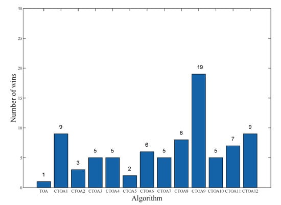
Figure 2. The number of wins for different algorithms in 30D.

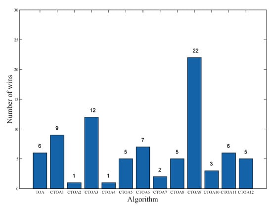
Figure 3. The number of wins for different algorithms in 50D.

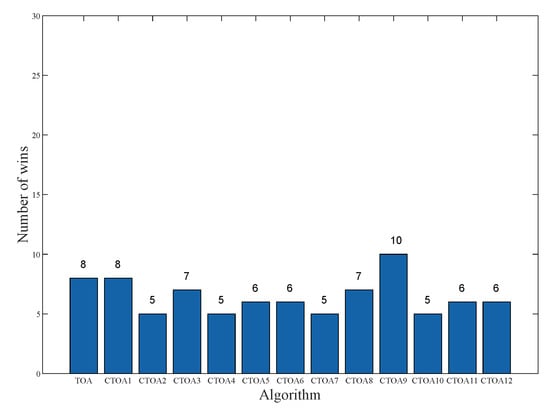
Figure 4. The number of wins for different algorithms in 100D.

The Friedman rank test is a nonparametric statistical test method. It is used to understand and compare overall rankings of algorithms. The Wilcoxon test is used to statistically compare the performance of two algorithms chosen to solve a particular problem. Table 20, Table 21 and Table 22 show the results of the Friedman ranking test for different algorithms in different dimensions. In the Friedman ranking, each algorithm obtains a Friedman Ranking, and the smaller the Friedman Ranking, the better the performance of the algorithm. From the tables, CTOA9 ranks first in both 30D and 50D, which means that the algorithm can achieve the best performance in these dimensions. Although CTOA9 did not obtain first place in Friedman’s ranking in 100D, the ranking is also very high, only a 6% difference from the optimal algorithm. The results of the Wilcoxon test are shown in Table 23. We selected a significance level of 0.05 and converted the weighted average of the evaluation indicators in the three dimensions into rank data. A p value < 0.05 indicates that the difference between the two algorithms is significant and the result is marked as 1. Except for CTOA3 and CTOA7, CTOA9 shows a significant difference compared to all other algorithms.

Table 20. Friedman ranking of different algorithms in 30D.

Algorithm	Friedman Ranking	Final Ranking
CTOA9	4.3	1
TOA	4.67	2
CTOA10	6.00	3
CTOA8	6.00	4
CTOA5	6.33	5
CTOA11	6.67	6
CTOA3	7.17	7
CTOA4	7.17	8
CTOA6	7.83	9
CTOA7	8.17	10
CTOA1	8.3	11
CTOA2	8.67	12
CTOA12	9.67	13

Table 21. Friedman ranking of different algorithms in 50D.

Algorithm	Friedman Ranking	Final Ranking
CTOA9	2.67	1
CTOA5	3.33	2
CTOA6	4.67	3
CTOA7	4.67	4
CTOA1	6.33	5
TOA	6.67	6
CTOA2	6.83	7
CTOA10	7.33	8
CTOA11	8.50	9
CTOA12	8.50	10
CTOA8	9.67	11
CTOA3	10.17	12
CTOA4	11.67	13

Table 22. Friedman ranking of different algorithms in 100D.

Algorithm	Friedman Ranking	Final Ranking
CTOA6	5.00	1
CTOA1	5.00	2
CTOA9	5.33	3
TOA	5.67	4
CTOA10	6.17	5
CTOA4	6.33	6
CTOA2	6.50	7
CTOA12	6.50	8
CTOA3	7	9
CTOA11	7.166666667	10
CTOA5	7.333333333	11
CTOA8	8.166666667	12
CTOA7	8.5	13

Table 23. The results of the Wilcoxon test.

Algorithm	Compared Algorithm	p Value	Result
CTOA9	TOA	0.0339	1
	CTOA1	0.0211	1
	CTOA2	0.0375	1
	CTOA3	0.0595	0
	CTOA4	0.0466	1
	CTOA5	0.0168	1
	CTOA6	0.0457	1
	CTOA7	0.0516	0
	CTOA8	0.4281	1
	CTOA10	0.0428	1
	CTOA11	0.0357	1
	CTOA12	0.2790	1

4.3. Experimental Results on Convergence

In this section, we run the CTOA presented in Table 4 at 30D, 50D, and 100D and record their convergence curves to demonstrate whether the CTOA algorithm has an advantage over the TOA in terms of convergence. Figure 5, Figure 6, Figure 7, Figure 8, Figure 9, Figure 10 and Figure 11 report the results of the algorithms in Table 4 running in 30D, Figure 12, Figure 13, Figure 14, Figure 15, Figure 16, Figure 17 and Figure 18 report the results in 50D, and Figure 19, Figure 20, Figure 21, Figure 22, Figure 23, Figure 24 and Figure 25 report the results in 100D. The best fitness value obtained by different algorithms on the benchmark function is used to evaluate the algorithm’s performance in terms of convergence speed during the iterative visualization process.

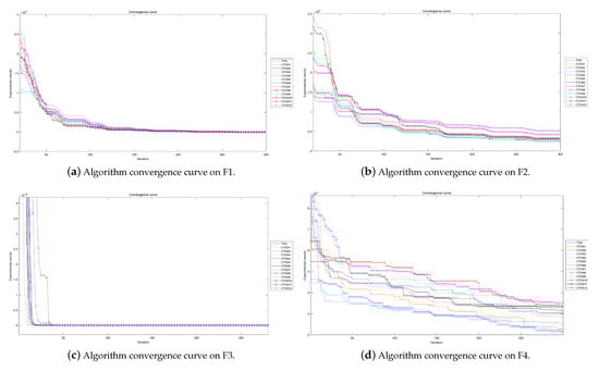
Figure 5. Algorithm convergence curves for benchmark functions F1–F4 run in 30D.

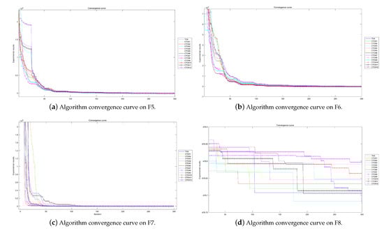
Figure 6. Algorithm convergence curves for benchmark functions F5–F8 run in 30D.

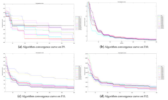
Figure 7. Algorithm convergence curves for benchmark functions F9–F12 run in 30D.

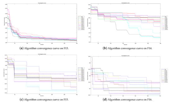
Figure 8. Algorithm convergence curves for benchmark functions F13–F16 run in 30D.

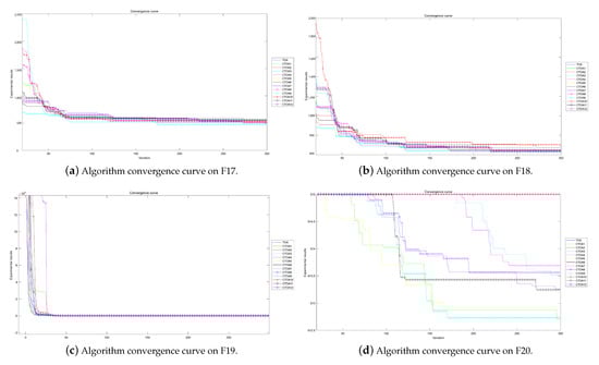
Figure 9. Algorithm convergence curves for benchmark functions F17–F20 run in 30D.

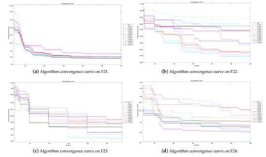
Figure 10. Algorithm convergence curves for benchmark functions F21–F24 run in 30D.

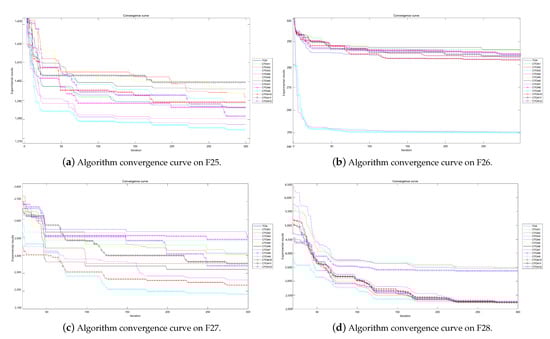
Figure 11. Algorithm convergence curves for benchmark functions F25–F28 run in 30D.

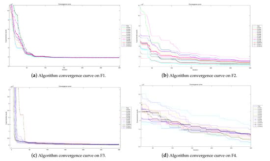
Figure 12. Algorithm convergence curves for benchmark functions F1–F4 run in 50D.

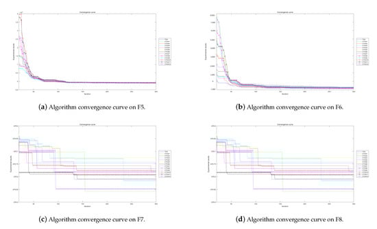
Figure 13. Algorithm convergence curves for benchmark functions F5–F8 run in 60D.

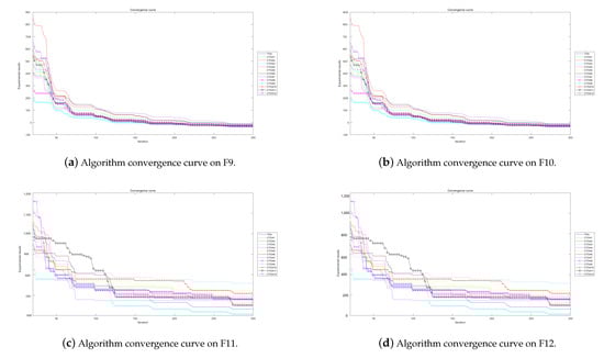
Figure 14. Algorithm convergence curves for benchmark functions F9–F12 run in 50D.

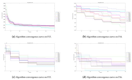
Figure 15. Algorithm convergence curves for benchmark functions F13–F16 run in 50D.

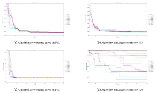
Figure 16. Algorithm convergence curves for benchmark functions F17–F20 run in 50D.

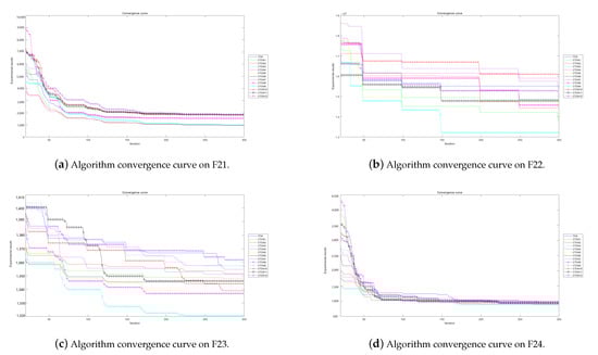
Figure 17. Algorithm convergence curves for benchmark functions F21–F24 run in 50D.

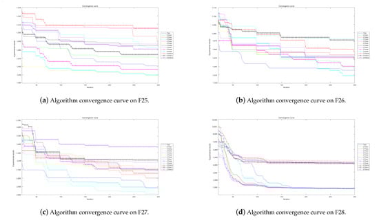
Figure 18. Algorithm convergence curves for benchmark functions F25–F28 run in 50D.

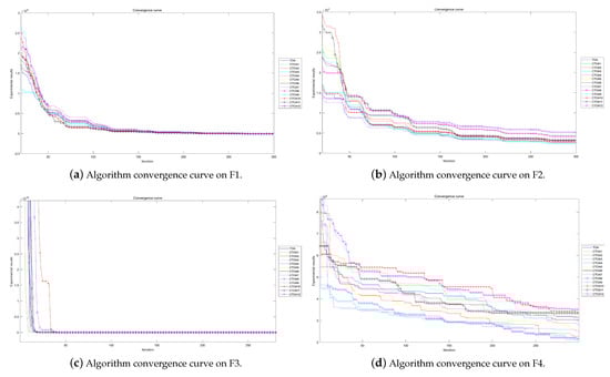
Figure 19. Algorithm convergence curves for benchmark functions F1–F4 run in 100D.

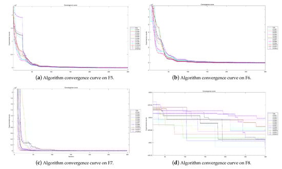
Figure 20. Algorithm convergence curves for benchmark functions F5–F8 run in 100D.

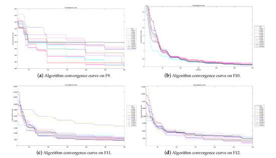
Figure 21. Algorithm convergence curves for benchmark functions F9–F12 run in 100D.

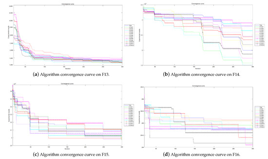
Figure 22. Algorithm convergence curves for benchmark functions F13–F16 run in 100D.

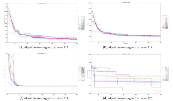
Figure 23. Algorithm convergence curves for benchmark functions F17–F20 run in 100D.

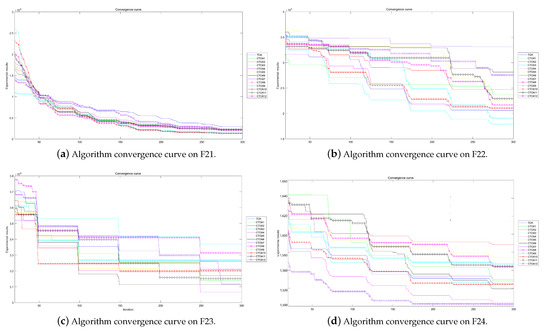
Figure 24. Algorithm convergence curves for benchmark functions F21–F24 run in 100D.

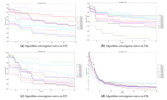
Figure 25. Algorithm convergence curves for benchmark functions F25–F28 run in 100D.

The experimental convergence curves also show that CTOA9 has obvious convergence compared to TOA and other algorithms using chaotic maps. CTOA9 achieves a faster convergence rate on most of the test functions, and after 300 iterations, the final fitness function results are also optimal. CTOA9 is not the fastest convergence speed in Figure 10d, Figure 13c and Figure 24a, but it is also faster than the other algorithms. On the unimodal function, there is only one global optimum of the benchmark function; thus, it is easier for the algorithm to search for the optimal position. Therefore, on the unimodal function F1–F5, all algorithms stagnate around iteration 150. On multimodal functions and composition functions, CTOA9 reaches the stagnation state later, and most algorithms reach the stagnation state before it, for example, at F8, F9, F14.

In addition, there is an “interesting” experimental phenomenon by observing the convergence curve of the CTOA9 algorithm running in 100D. That is, the convergence curves become similar, such as in Figure 19a,c and Figure 20b which means that the performance of CTOA and TOA in convergence tends to be consistent.

4.4. Comparison with State-of-the-Art Algorithms

From previous experiments, we can prove that CTOA9 is the best among all CTOAs. To accurately evaluate and draw conclusions regarding the quality of the proposed algorithm in terms of stagnation, exploration, and diversity, we conducted experiments to compare other algorithms of the same type. Therefore, we selected GA [3], PSO [2], ACO [7], and SFLA [8] and compared them with CTOA9. According to previous studies, the algorithm parameter settings are shown in Table 24.

Table 24. The parameter settings for the relevant algorithm.

Algorithm	Parameter	Description
CTOA9	$gc$ = 50	seed growth cycle
GA [3]	$pm$ = 0.005	mutation rate
	$pc$ = 0.7	crossover rate
PSO [2]	$c_1$ = $c_2$ = 1	learning factor
	w = 0.9	weight
	$vmax$ = 6	maximum velocity limit
ACO [7]	$rho$ = 0.2	pheromone volatilization speed
SFLA [8]	q = 2	number of parents
	$\alpha$ = 3	number of offsprings
	$\beta$ = 5	maximum number of iterations
	$\sigma$ = 2	step size
	$nMemeplex$ = 5	number of memeplexes

We selected some benchmark functions, and the convergence speeds of the algorithm on these functions are shown in Figure 26, Figure 27 and Figure 28. On the unimodal functions F1, F2, F5, SFLA has the fastest convergence speed and the best fitness value. After about 50 iterations, CTOA9 converged and then stagnated. Among these algorithms, SFLA has the best performance on unimodal functions, and CTOA9 is slightly weaker than it. On multimodal functions F9–F14, CTOA9 stagnates after 700 iterations except for F9 and F10. GA and SFLA can converge in less than 100 iterations, but their fitness values are very poor. Although the convergence speed of CTOA is slow, the final fitness value is optimal among all algorithms. Similarly, CTOA9 also obtains the best fitness value on the mixture function F21–F23. In summary, although the convergence speed of CTOA9 is slow, it has a strong global exploration ability, can jump out of the local optimum, and continuously updates the optimal value.

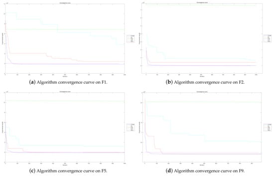
Figure 26. Algorithm convergence curves for benchmark functions.

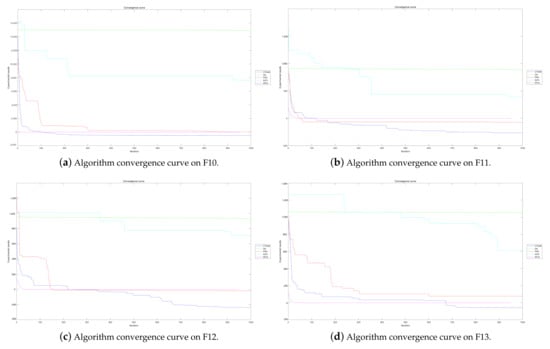
Figure 27. Algorithm convergence curves for benchmark functions.

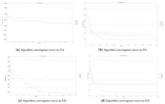
Figure 28. Algorithm convergence curves for benchmark functions.

Nonparametric statistical methods can help us compare the performance of different algorithms. Therefore, we conducted a Friedman test and Wilcoxon signed-rank test on CTOA9, GA, PSO, ACO, SFLA, and statistical values were obtained on the benchmark functions. The results of the Friedman test are shown in Table 25. The results of the Wilcoxon signed-rank test are shown in Table 26. From Table 25, CTOA can achieve the best performance in the Friedman test. SFLA performance is slightly weaker than CTOA9. GA was the worst performer, ranking fifth. In addition, through Table 26, CTOA9 is significantly different from all other algorithms. In summary, through nonparametric statistical experiments, CTOA9 is the best in terms of overall performance.

Table 25. Friedman ranking of different algorithms.

Algorithm	Friedman Ranking	Final Ranking
CTOA9	2.46	1
SFLA [8]	3.17	2
PSO [2]	3.33	3
ACO [7]	4.75	4
GA [3]	5	5

Table 26. The results of the Wilcoxon test comparing CTOA with state-of-the art algorithms.

Algorithm	Compared Algorithm	p-Value	Result
CTOA9	SFLA [8]	0.0133	1
	ACO [7]	0.0355	1
	PSO [2]	0.0407	1
	GA [3]	0.0403	1

5. Real Problem: Power Generation Prediction

With the rapid development of the economy, people’s electricity consumption has increased, such that the huge electricity load has increased the requirements for power generation. Power generation prediction is critical for accurate decision making by electric utilities and power plants. For the feature data collected from the power plant, the relationship between each parameter is mutually influenced, and many features cannot be expressed by a simple functional relationship. Support vector machine (SVM) is a commonly used machine learning algorithm. The SVM model has unique advantages in reflecting the nonlinear relationship between parameters. The performance of SVM largely depends on the values of the selected hyperparameters. The penalty parameter c and the width parameter g play a decisive role in the classification results and prediction accuracy of SVM.

Cross-validation is often used to select hyperparameters, but this approach tends to consume a lot of computational resources and time. Because the metaheuristic algorithm performs well in random searches and iterations in the hyperparameter space, it is widely used in the hyperparameter optimization of SVM. The proposed CTOA algorithm can help us find the best combination of hyperparameters. To examine the performance of the proposed algorithm, we applied the proposed algorithm to an optimized power forecasting model and compared the results of the proposed optimal CTOA9 with GA, PSO, ACO, SFLA ACO. According to previous studies, the algorithm parameter settings are shown in Table 24.

The framework of this method is shown in Figure 29.

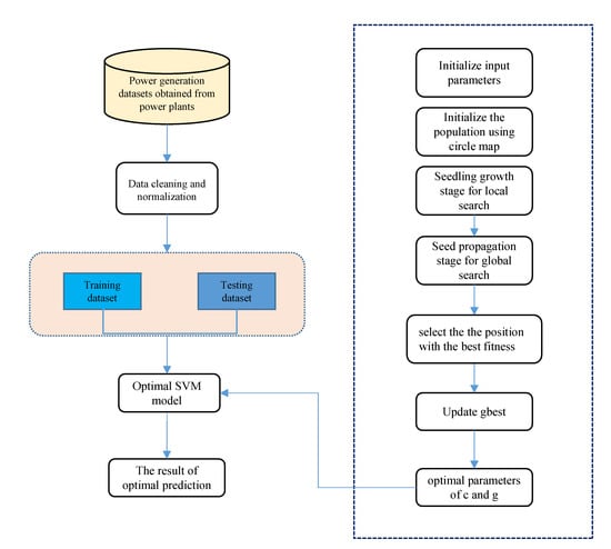
Figure 29. The framework of the power prediction model.

Additionally, the prediction error used as the fitness function in this problem is shown in the following equation:

$$Fitness=\sqrt{\frac{1}{m}\sum _{i=1}^{N_p}{\left|y_i-{\widehat{y}}_i\right|}^2}$$

(12)

where m is the total number of training samples, and $y_i$ and ${\widehat{y}}_i$ are the actual and model predicted values. In order to evaluate the model more comprehensively, we also used $R^2$ as the evaluation standard, and its equation is shown below:

$$R^2=1-\frac{{\sum }_i{\left({\widehat{y}}_i-y_i\right)}^2}{{\sum }_i{\left({\overline{y}}_i-y_i\right)}^2}$$

(13)

where $y_i$ is the true value, and $\widehat{y}$ is the predicted value.

All algorithms were used to optimize SVM parameters and are applied in power forecasting, and the obtained results are shown in the Table 27. Among the two selected evaluation indicators, the smaller RMSE is better, and the closer $R^2$ is to 1, the better. The final RMSE obtained by CTOA = 0.051033, which is the best among the six algorithms, 7.4% higher than the second PSO algorithm. The final $R^2$ = 0.96719 obtained by CTOA is very close to 1. It performs best among all algorithms. In summary, the newly proposed CTOA-SVM model performs best.

Table 27. The results of different algorithms.

Algorithm	RMSE	${\mathit{R}}^2$
CTOA9	0.051033	0.96719
SFLA [8]	0.051071	0.95767
ACO [7]	0.051573	0.92724
PSO [2]	0.051572	0.92623
GA [3]	0.051655	0.93110

6. Discussion

The experimental results demonstrate that the use of chaotic maps improves the performance of TOA in solving optimization problems. Specifically, the numerical statistics and convergence speed of CTOA are significantly better than that of TOA. The circle map is observed to have the most prominent effect on improving the algorithm’s performance, particularly in 50D. When the population position is initialized, the chaotic sequence generated by the circle map is used to replace the random initial sequence, which makes the population evenly distributed and expands the global search range. However, as the dimensions increase, the performance of TOA also improves, and its performance is comparable to that of CTOA in 100D. This implies that the advantages of using chaotic maps to improve TOA’s performance diminish in higher dimensions, and the performance of both TOA and CTOA tends to become average. This suggests that CTOA is more suited for optimization problems at lower dimensions, specifically in the range of 30–50D. Moreover, the increase in the number of variables in higher dimensions makes it difficult for chaotic maps to handle such complexity, leading to a reduction in performance improvement. Although CTOA9 is not significant to CTOA3 and CTOA7, it does not imply that CTOA9 performs poorly in the Wilcoxon test experiment. The Wilcoxon rank sum test is just a statistical method used to compare the differences between two samples, and its results are affected by many factors, which need to be fully considered in future research. In the convergence results, the fitness value of CTOA9 is still being updated, indicating that the algorithm still has more exploration capabilities when the iteration terminates ($Max\_itertion=300$). In future research, it is necessary to increase the number of iterations so that the algorithm converges eventually, to fully evaluate the convergence speed.

7. Conclusions

In this paper, we presented a novel optimization algorithm called the chaotic-based tumbleweed optimization algorithm (CTOA). The use of chaotic maps increases the diversity of the initial population, leading to improved algorithm performance. The performance of CTOA was tested on 28 benchmark functions of CEC2013. The comparative experimental results showed that the improved CTOA using the circle map is better than the original TOA in both the accuracy and convergence speed of finding the optimal value. We conclude that the CTOA9 algorithm using the circle map outperforms other CTOAs and TOA in terms of optimal results and benchmark function convergence. We compared CTOA9 with famous state-of-the-art optimization algorithms, including GA, PSO, ACO, SFLA. The results demonstrated that CTOA9 is not only best on the Friedman ranking test and Wilcoxon test, but it also has the minimum error when applied to power generation prediction problems. In addition, the performance of CTOA based on a circle map is more outstanding in lower search space dimensions (30D and 50D), but as the dimension increases to 100D, the performance of CTOA and TOA become more similar. Therefore, the CTOA algorithm is more suitable for solving problems with lower search space dimensions.

References

- Zhang, F.; Wu, T.Y.; Wang, Y.; Xiong, R.; Ding, G.; Mei, P.; Liu, L. Application of quantum genetic optimization of LVQ neural network in smart city traffic network prediction. IEEE Access 2020, 8, 104555–104564. [Google Scholar] [CrossRef]
- Marini, F.; Walczak, B. Particle swarm optimization (PSO). A tutorial. Chemom. Intell. Lab. Syst. 2015, 149, 153–165. [Google Scholar] [CrossRef]
- Mirjalili, S. Genetic Algorithm. In Evolutionary Algorithms and Neural Networks: Theory and Applications; Springer International Publishing: Cham, Switzerland, 2019; pp. 43–55. [Google Scholar] [CrossRef]
- Nasiri, J.; Khiyabani, F.M. A whale optimization algorithm (WOA) approach for clustering. Cogent Math. Stat. 2018, 5, 1483565. [Google Scholar] [CrossRef]
- Mirjalili, S.; Mirjalili, S.M.; Lewis, A. Grey Wolf Optimizer. Adv. Eng. Softw. 2014, 69, 46–61. [Google Scholar] [CrossRef]
- Mirjalili, S.; Gandomi, A.H.; Mirjalili, S.Z.; Saremi, S.; Faris, H.; Mirjalili, S.M. Salp Swarm Algorithm: A bio-inspired optimizer for engineering design problems. Adv. Eng. Softw. 2017, 114, 163–191. [Google Scholar] [CrossRef]
- Kumar, S.; Kumar-Solanki, V.; Kumar Choudhary, S.; Selamat, A.; González-Crespo, R. Comparative Study on Ant Colony Optimization (ACO) and K-Means Clustering Approaches for Jobs Scheduling and Energy Optimization Model in Internet of Things (IoT); ACM: New York, NY, USA, 2020. [Google Scholar]
- Eusuff, M.; Lansey, K.; Pasha, F. Shuffled frog-leaping algorithm: A memetic meta-heuristic for discrete optimization. Eng. Optim. 2006, 38, 129–154. [Google Scholar] [CrossRef]
- Chen, J.; Jiang, J.; Guo, X.; Tan, L. A self-Adaptive CNN with PSO for bearing fault diagnosis. Syst. Sci. Control Eng. 2021, 9, 11–22. [Google Scholar] [CrossRef]
- Malviya, S.; Kumar, P.; Namasudra, S.; Tiwary, U.S. Experience Replay-Based Deep Reinforcement Learning for Dialogue Management Optimisation; ACM: New York, NY, USA, 2022. [Google Scholar]
- Houssein, E.H.; Saad, M.R.; Hussain, K.; Zhu, W.; Shaban, H.; Hassaballah, M. Optimal Sink Node Placement in Large Scale Wireless Sensor Networks Based on Harris’ Hawk Optimization Algorithm. IEEE Access 2020, 8, 19381–19397. [Google Scholar] [CrossRef]
- Singh, P.; Chaudhury, S.; Panigrahi, B.K. Hybrid MPSO-CNN: Multi-level particle swarm optimized hyperparameters of convolutional neural network. Swarm Evol. Comput. 2021, 63, 100863. [Google Scholar] [CrossRef]
- Wu, T.Y.; Li, H.; Chu, S.C. CPPE: An Improved Phasmatodea Population Evolution Algorithm with Chaotic Maps. Mathematics 2023, 11, 1977. [Google Scholar] [CrossRef]
- Shaik, A.L.H.P.; Manoharan, M.K.; Pani, A.K.; Avala, R.R.; Chen, C.M. Gaussian Mutation–Spider Monkey Optimization (GM-SMO) Model for Remote Sensing Scene Classification. Remote Sens. 2022, 14, 6279. [Google Scholar] [CrossRef]
- Xue, X.; Guo, J.; Ye, M.; Lv, J. Similarity Feature Construction for Matching Ontologies through Adaptively Aggregating Artificial Neural Networks. Mathematics 2023, 11, 485. [Google Scholar] [CrossRef]
- Li, D.; Xiao, P.; Zhai, R.; Sun, Y.; Wenbin, H.; Ji, W. Path Planning of Welding Robots Based on Developed Whale Optimization Algorithm. In Proceedings of the 2021 6th International Conference on Control, Robotics and Cybernetics (CRC), Shanghai, China, 9–11 October 2021; pp. 101–105. [Google Scholar] [CrossRef]
- Chen, C.M.; Lv, S.; Ning, J.; Wu, J.M.T. A Genetic Algorithm for the Waitable Time-Varying Multi-Depot Green Vehicle Routing Problem. Symmetry 2023, 15, 124. [Google Scholar] [CrossRef]
- Chuang, L.Y.; Chang, H.W.; Tu, C.J.; Yang, C.H. Improved binary PSO for feature selection using gene expression data. Comput. Biol. Chem. 2008, 32, 29–38. [Google Scholar] [CrossRef] [PubMed]
- Xue, X. Complex ontology alignment for autonomous systems via the Compact Co-Evolutionary Brain Storm Optimization algorithm. ISA Trans. 2023, 132, 190–198. [Google Scholar] [CrossRef] [PubMed]
- Huang, C.L.; Wang, C.J. A GA-based feature selection and parameters optimizationfor support vector machines. Expert Syst. Appl. 2006, 31, 231–240. [Google Scholar] [CrossRef]
- Ziadeh, A.; Abualigah, L.; Elaziz, M.A.; Şahin, C.B.; Almazroi, A.A.; Omari, M. Augmented grasshopper optimization algorithm by differential evolution: A power scheduling application in smart homes. Multimed. Tools Appl. 2021, 80, 31569–31597. [Google Scholar] [CrossRef]
- Sheikholeslami, R.; Kaveh, A.a. A Survey of chaos embedded meta-heuristic algorithms. Int. J. Optim. Civ. Eng. 2013, 3, 617–633. [Google Scholar]
- Rajabioun, R. Cuckoo optimization algorithm. Appl. Soft Comput. 2011, 11, 5508–5518. [Google Scholar] [CrossRef]
- Bastos Filho, C.J.A.; de Lima Neto, F.B.; Lins, A.J.C.C.; Nascimento, A.I.S.; Lima, M.P. A novel search algorithm based on fish school behavior. In Proceedings of the 2008 IEEE International Conference on Systems, Man and Cybernetics, Singapore, 12–15 October 2008; pp. 2646–2651. [Google Scholar] [CrossRef]
- Wang, H.; Wu, Z.; Rahnamayan, S.; Liu, Y.; Ventresca, M. Enhancing particle swarm optimization using generalized opposition-based learning. Inf. Sci. 2011, 181, 4699–4714. [Google Scholar] [CrossRef]
- Li, W.; Wang, G.G. Improved elephant herding optimization using opposition-based learning and K-means clustering to solve numerical optimization problems. J. Ambient Intell. Humaniz. Comput. 2023, 14, 1753–1784. [Google Scholar] [CrossRef]
- Khamkar, R.; Das, P.; Namasudra, S. SCEOMOO: A novel Subspace Clustering approach using Evolutionary algorithm, Off-spring generation and Multi-Objective Optimization. Appl. Soft Comput. 2023, 139, 110185. [Google Scholar] [CrossRef]
- Bajer, D.; Martinović, G.; Brest, J. A population initialization method for evolutionary algorithms based on clustering and Cauchy deviates. Expert Syst. Appl. 2016, 60, 294–310. [Google Scholar] [CrossRef]
- Poikolainen, I.; Neri, F.; Caraffini, F. Cluster-Based Population Initialization for differential evolution frameworks. Inf. Sci. 2015, 297, 216–235. [Google Scholar] [CrossRef]
- Chuang, L.Y.; Hsiao, C.J.; Yang, C.H. Chaotic particle swarm optimization for data clustering. Expert Syst. Appl. 2011, 38, 14555–14563. [Google Scholar] [CrossRef]
- Wang, Y.; Liu, H.; Ding, G.; Tu, L. Adaptive chimp optimization algorithm with chaotic map for global numerical optimization problems. J. Supercomput. 2022, 79, 6507–6537. [Google Scholar] [CrossRef]
- Gao, W.f.; Liu, S.y.; Huang, L.l. Particle swarm optimization with chaotic opposition-based population initialization and stochastic search technique. Commun. Nonlinear Sci. Numer. Simul. 2012, 17, 4316–4327. [Google Scholar] [CrossRef]
- Yang, J.; Liu, Z.; Zhang, X.; Hu, G. Elite Chaotic Manta Ray Algorithm Integrated with Chaotic Initialization and Opposition-Based Learning. Mathematics 2022, 10, 2960. [Google Scholar] [CrossRef]
- Gandomi, A.H.; Yun, G.J.; Yang, X.S.; Talatahari, S. Chaos-enhanced accelerated particle swarm optimization. Commun. Nonlinear Sci. Numer. Simul. 2013, 18, 327–340. [Google Scholar] [CrossRef]
- Arora, S.; Singh, S. An improved butterfly optimization algorithm with chaos. J. Intell. Fuzzy Syst. 2017, 32, 1079–1088. [Google Scholar] [CrossRef]
- Kohli, M.; Arora, S. Chaotic grey wolf optimization algorithm for constrained optimization problems. J. Comput. Des. Eng. 2018, 5, 458–472. [Google Scholar] [CrossRef]
- Jia, D.; Zheng, G.; Khan, M.K. An effective memetic differential evolution algorithm based on chaotic local search. Inf. Sci. 2011, 181, 3175–3187. [Google Scholar] [CrossRef]
- Pan, J.S.; Yang, Q.; Shieh, C.S.; Chu, S.C. Tumbleweed Optimization Algorithm and Its Application in Vehicle Path Planning in Smart City. J. Internet Technol. 2022, 23, 927–945. [Google Scholar]
- Sayed, G.I.; Darwish, A.; Hassanien, A.E. A new chaotic multi-verse optimization algorithm for solving engineering optimization problems. J. Exp. Theor. Artif. Intell. 2018, 30, 293–317. [Google Scholar] [CrossRef]
- Du, T.S.; Ke, X.T.; Liao, J.G.; Shen, Y.J. DSLC-FOA: Improved fruit fly optimization algorithm for application to structural engineering design optimization problems. Appl. Math. Model. 2018, 55, 314–339. [Google Scholar] [CrossRef]
- Tharwat, A.; Elhoseny, M.; Hassanien, A.E.; Gabel, T.; Kumar, A. Intelligent Bézier curve-based path planning model using Chaotic Particle Swarm Optimization algorithm. Clust. Comput. 2019, 22, 4745–4766. [Google Scholar] [CrossRef]
- Kaveh, A.; Mahdipour Moghanni, R.; Javadi, S. Optimum design of large steel skeletal structures using chaotic firefly optimization algorithm based on the Gaussian map. Struct. Multidiscip. Optim. 2019, 60, 879–894. [Google Scholar] [CrossRef]
- Demidova, L.A.; Gorchakov, A.V. A study of chaotic maps producing symmetric distributions in the fish school search optimization algorithm with exponential step decay. Symmetry 2020, 12, 784. [Google Scholar] [CrossRef]
- Li, Y.; Han, M.; Guo, Q. Modified whale optimization algorithm based on tent chaotic mapping and its application in structural optimization. KSCE J. Civ. Eng. 2020, 24, 3703–3713. [Google Scholar] [CrossRef]
- Agrawal, P.; Ganesh, T.; Mohamed, A.W. Chaotic gaining sharing knowledge-based optimization algorithm: An improved metaheuristic algorithm for feature selection. Soft Comput. 2021, 25, 9505–9528. [Google Scholar] [CrossRef]
- Li, X.D.; Wang, J.S.; Hao, W.K.; Zhang, M.; Wang, M. Chaotic arithmetic optimization algorithm. Appl. Intell. 2022, 52, 16718–16757. [Google Scholar] [CrossRef]
- Onay, F.K.; Aydemir, S.B. Chaotic hunger games search optimization algorithm for global optimization and engineering problems. Math. Comput. Simul. 2022, 192, 514–536. [Google Scholar] [CrossRef]
- Yang, P.; Wang, T.; Yang, H.; Meng, C.; Zhang, H.; Cheng, L. The Performance of Electronic Current Transformer Fault Diagnosis Model: Using an Improved Whale Optimization Algorithm and RBF Neural Network. Electronics 2023, 12, 1066. [Google Scholar] [CrossRef]
- Chaoxi, L.; Lifang, H.; Songwei, H.; Bin, H.; Changzhou, Y.; Lingpan, D. An improved bald eagle algorithm based on Tent map and Levy flight for color satellite image segmentation. Signal Image Video Process. 2023, 1–9. [Google Scholar] [CrossRef]
- Naik, A. Chaotic Social Group Optimization for Structural Engineering Design Problems. J. Bionic Eng. 2023, 1–26. [Google Scholar] [CrossRef]
- Phatak, S.C.; Rao, S.S. Logistic map: A possible random-number generator. Phys. Rev. E 1995, 51, 3670–3678. [Google Scholar] [CrossRef]
- Devaney, R.L. A piecewise linear model for the zones of instability of an area-preserving map. Phys. D Nonlinear Phenom. 1984, 10, 387–393. [Google Scholar] [CrossRef]
- Ibrahim, R.A.; Oliva, D.; Ewees, A.A.; Lu, S. Feature selection based on improved runner-root algorithm using chaotic singer map and opposition-based learning. In Proceedings of the International Conference on Neural Information Processing, Long Beach, CA, USA, 4–9 December 2017; pp. 156–166. [Google Scholar]
- Hua, Z.; Zhou, Y. Image encryption using 2D Logistic-adjusted-Sine map. Inf. Sci. 2016, 339, 237–253. [Google Scholar] [CrossRef]
- Driebe, D.J. The bernoulli map. In Fully Chaotic Maps and Broken Time Symmetry; Springer: Berlin/Heidelberg, Germany, 1999; pp. 19–43. [Google Scholar]
- Jensen, M.H.; Bak, P.; Bohr, T. Complete devil’s staircase, fractal dimension, and universality of mode-locking structure in the circle map. Phys. Rev. Lett. 1983, 50, 1637. [Google Scholar] [CrossRef]
- Rogers, T.D.; Whitley, D.C. Chaos in the cubic mapping. Math. Model. 1983, 4, 9–25. [Google Scholar] [CrossRef]
- Sayed, G.I.; Darwish, A.; Hassanien, A.E. A new chaotic whale optimization algorithm for features selection. J. Classif. 2018, 35, 300–344. [Google Scholar] [CrossRef]
- Liu, W.; Sun, K.; He, Y.; Yu, M. Color image encryption using three-dimensional sine ICMIC modulation map and DNA sequence operations. Int. J. Bifurc. Chaos 2017, 27, 1750171. [Google Scholar] [CrossRef]
- Li, X.; Engelbrecht, A.; Epitropakis, M.G. Benchmark Functions for CEC’2013 Special Session and Competition on Niching Methods for Multimodal Function Optimization; RMIT University, Evolutionary Computation and Machine Learning Group: Melbourne, Australia, 2013. [Google Scholar]
Disclaimer/Publisher’s Note: The statements, opinions and data contained in all publications are solely those of the individual author(s) and contributor(s) and not of MDPI and/or the editor(s). MDPI and/or the editor(s) disclaim responsibility for any injury to people or property resulting from any ideas, methods, instructions or products referred to in the content. |
© 2023 by the authors. Licensee MDPI, Basel, Switzerland. This article is an open access article distributed under the terms and conditions of the Creative Commons Attribution (CC BY) license (https://creativecommons.org/licenses/by/4.0/).