The Slashed Power Half-Normal Distribution with Applications

Abstract

In this paper, an extension of the power half-normal (PHN) distribution is introduced. This new model is built on the application of slash methodology for positive random variables. The result is a distribution with greater kurtosis than the PHN; i.e., its right tail is heavier than the PHN distribution. Its probability density, survival and hazard rate function are studied, and moments, skewness and kurtosis coefficientes are obtained, along with relevant properties of interest in reliability. It is also proven that the new model can be expressed as the scale mixture of a PHN and a uniform distribution. Moreover, the new model holds the PHN distribution as a limit case when the new parameter tends to infinity. The parameters in the model are estimated by the method of moments and maximum likelihood. A simulation study is given to illustrate the good behavior of maximum likelihood estimators. Two real applications to survival and fatigue fracture data are included, in which our proposal outperforms other models.

1. Introduction

The half-normal (HN) distribution is suitable to fit positive data. For this reason, it is of interest in reliability and survival analysis as a lifetime model. The HN model also exhibits a large number of theoretical properties; for instance, it can be obtained as a particular case of the folded normal, the truncated normal, or the central chi distribution with one degree of freedom; details can be seen in Johnson et al. [1]. Recall that a random variable (rv) Z follows an HN distribution with scale parameter $\sigma >0$, $Z\sim HN\left(\sigma \right)$ if its probability density function (pdf) is given by

$$f(z;\sigma )=\frac{2}{\sigma }\varphi \left(\frac{z}{\sigma }\right),z>0,$$

where $\sigma >0$ and $\varphi (·)$ denotes the pdf of a $N(0,1)$ distribution.

Properties of the HN distribution and first applications can be seen in the papers by Rogers and Tukey [2] and Mosteller and Tukey [3]. Pewsey [4,5] introduced the general location-scale HN distribution and studied asymptotic inference based on maximum likelihood (ML) estimators. Later, Wiper et al. [6] obtained Bayesian results in the general HN and half-t distributions. Cooray and Ananda [7] proposed the generalized half-normal (GHN) distribution as a lifetime model useful for items subjects to static fatigue. Ahmadi and Yousefzadeh [8] obtained results in the GHN for type I interval censoring data. Olmos et al. [9,10] used the slash methodology to extend the HN and GHN distributions. They proposed models with more kurtosis than their precedents.

On the other hand, Gómez and Bolfarine [11] introduced the two-parameter PHN distribution. This is a model useful to fit positive data with a shape parameter, which provides flexibility to the pdf, survival, and hazard rate function with respect to the HN distribution. They also showed that the PHN model is a competitor of the GHN model, and therefore, it can be used as a static fatigue lifetime model. Due to its good properties, the PHN will be the starting point to introduce our proposal. Our aim is to get the slashed version of the PHN model.

Next, we recall the main features of the PHN model (see [11]). It is said that an rv X follows a PHN distribution, $X\sim PHN(\sigma ,\alpha )$, if its pdf is given by

$$g_X(x;\sigma ,\alpha )=\frac{2\alpha }{\sigma }\varphi \left(\frac{x}{\sigma }\right){\left(2\Phi \left(\frac{x}{\sigma }\right)-1\right)}^{\alpha -1},x>0,$$

where $\sigma >0$ and $\alpha >0$ are scale and shape parameters, respectively, and $\Phi (·)$ denotes the cumulative distribution function (cdf) of a $N(0,1)$.

Lemma 1

(Properties of PHN distribution, [11]). Let $X\sim PHN(\sigma ,\alpha )$. Then

1. 

The cdf of X is

$$G_X(x;\sigma ,\alpha )={\left(2\Phi \left(\frac{x}{\sigma }\right)-1\right)}^{\alpha },x>0.$$

(1)

2. 

The rth-moment is

$$E\left(X^r\right)=\alpha {\sigma }^r{\kappa }_r\left(\alpha \right),\mathit{for}r=1,2,\dots ,$$

(2)

with

$${\kappa }_r={\kappa }_r\left(\alpha \right)={\int }_0^1{\left({\Phi }^{-1}\left(\frac{1+u}{2}\right)\right)}^r{u}^{\alpha -1}du.$$

(3)

3. 

In particular

(a) 

$E\left(X\right)=\alpha \sigma {\kappa }_1$.

(b) 

$Var\left(X\right)=\alpha {\sigma }^2\left({\kappa }_2-\alpha {\kappa }_1^2\right)$.

(c) 

Skewness coefficient, defined as $\sqrt{{\beta }_{1,X}}=\frac{E\left[{(X-E\left[X\right])}^3\right]}{{\left(Var\left(X\right)\right)}^{3/2}}$, is

$$\sqrt{{\beta }_{1,X}}=\frac{{\kappa }_3-3\alpha {\kappa }_1{\kappa }_2+2{\alpha }^2{\kappa }_1^3}{\sqrt{\alpha }{({\kappa }_2-\alpha {\kappa }_1^2)}^{3/2}}.$$

(4)

(d) 

Kurtosis coefficient, defined as ${\beta }_{2,X}=\frac{E\left[{(X-E\left[X\right])}^4\right]}{{\left(Var\left(X\right)\right)}^2}$, is

$${\beta }_{2,X}=\frac{{\kappa }_4-4\alpha {\kappa }_1{\kappa }_3+6{\alpha }^2{\kappa }_1^2{\kappa }_2-3{\alpha }^2{\kappa }_1^4}{\alpha {({\kappa }_2-\alpha {\kappa }_1^2)}^2}.$$

(5)

It can be seen in [11] that $\sqrt{{\beta }_{1,X}}$ and ${\beta }_{2,X}$ are decreasing functions of $\alpha$. The aim of this paper is to propose an extension of the PHN model whose kurtosis coefficient exhibits a greater range of values than the kurtosis coefficient in the PHN model, and therefore, it may be used to accommodate outlying observations.

In this sense, it is well known that the slash models have heavier tails than other classical distributions, such as the normal one. Relevant papers, which illustrate the main properties of slash models, are Segovia et al. [12], Wang et al. [13] and Iriarte et al. [14].

The outline of this paper is as follows. In Section 2, the stochastic representation of the slash power half-normal (SPHN) model is given, its pdf, cdf, properties, relationships and approximations to other models, expression as a mixture, moments, asymmetry and kurtosis coefficients, and stochastic ordering properties are studied. In Section 3, given a random sample of the SPHN model, inference for the unknown parameters is carried out by using moment and maximum likelihood methods. In Section 4, a simulation study is carried out. An algorithm to generate random values in the SPHN model is proposed, and the consistency of ML estimators is analyzed there. In Section 5, two real applications dealing with survival and fatigue fracture data are given. In this section, our model is compared to other competing models, such as PHN, GHN, Slash Power Maxwell (see [12]), LogNormal and slash generalized half-normal (SGHN) (see [10]). It is proven that our proposal outperforms the competitors. Finally, a brief discussion, some conclusions and future tasks are given in Section 6.

2. The Slashed Power Half-Normal Distribution

In this section, the new model is introduced, and its theoretical properties are studied. First, the stochastic representation of the SPHN model is given; that is, a continuous, non-negative rv T follows a SPHN distribution, $T\sim SPHN(\sigma ,\alpha ,q)$, if T is obtained as

$$T=\frac{X}{Y^{1/q}}$$

(6)

where $X\sim PHN(\sigma ,\alpha )$ and $Y\sim U(0,1)$ are independent, $\sigma >0$, $\alpha >0$, and $q>0$.

In (6), $\sigma >0$ is a scale parameter, whereas $\alpha >0$ and $q>0$ are shape parameters. It will be seen in Section 2.3 that q increases the range of possible values for the kurtosis coefficient in the SPHN model with respect to the PHN distribution. In the next proposition, the pdf of (6) is obtained.

Proposition 1.

Let $T\sim SPHN(\sigma ,\alpha ,q)$. Then, the pdf of T is given by

$$f_T(t;\sigma ,\alpha ,q)=\frac{{\sigma }^q\alpha q}{t^{q+1}}{M}_{\alpha ,q}\left(2\Phi \left(\frac{t}{\sigma }\right)-1\right),t>0,$$

(7)

where $\sigma >0$,  $\alpha >0$, $q>0$, and

$${\displaystyle M_{\alpha ,q}\left(r\right)={\int }_0^r{\left[{\Phi }^{-1}\left(\frac{1+u}{2}\right)\right]}^q{u}^{\alpha -1}du.}$$

(8)

Proof. 

By using (6), the Jacobian technique, and marginalizing, the pdf of T is given by

$$f_T(t;\sigma ,\alpha ,q)=\frac{2\alpha q}{\sigma }{\int }_0^1{w}^q\varphi \left(\frac{tw}{\sigma }\right){\left(2\Phi \left(\frac{tw}{\sigma }\right)-1\right)}^{\alpha -1}dw.$$

Making the change of variable $r=\frac{tw}{\sigma }$, we have

$$\begin{array}{cc}{f}_T(t;\sigma ,\alpha ,q)& =\frac{2{\sigma }^q\alpha q}{t^{q+1}}{\int }_0^{t/\sigma }{r}^q\varphi \left(r\right){\left(2\Phi \left(r\right)-1\right)}^{\alpha -1}dr.\end{array}$$

Finally, by considering the change of variable $u=2\Phi \left(r\right)-1$, (7) is obtained. □

Figure 1 shows the pdf of the SPHN model for fixed values of $\sigma =1$, $\alpha =2$, and several values of parameter $q>0$. This plot suggests that the right tail in this model becomes heavier as q becomes smaller.

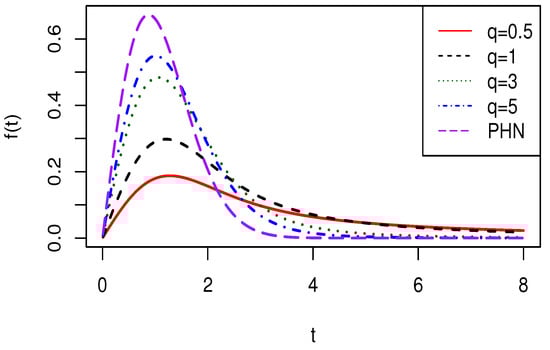
Figure 1. Plots of the SPHN($1,2,q$) model.

Moreover, Table 1 compares the right tail in the PHN and SPHN distributions for several values of q, $q\in \{0.5,1,5,10\}$. Note that for a fixed t value, the closer to zero q is, the greater $P(T>t)$ is obtained. These appreciations agree with the fact that q is mainly related to the kurtosis in this new model, as it will be seen in Section 2.3.

Table 1. Right tail comparison for different SPHN and PHN distributions.

Distribution	$\mathit{P}(\mathit{T}>3)$	$\mathit{P}(\mathit{T}>4)$	$\mathit{P}(\mathit{T}>5)$
SPHN (1, 2, 0.5)	$0.5895$	$0.5107$	$0.4568$
SPHN (1, 2, 1)	$0.3756$	$0.2821$	$0.2257$
SPHN (1, 2, 5)	$0.0462$	$0.0118$	$0.0039$
SPHN (1, 2, 10)	$0.0173$	$0.0017$	$0.0002$
PHN (1, 2)	$0.0054$	$1.26\times {10}^{-4}$	$1.14\times {10}^{-6}$

Remark 1.

For completeness, plots of the pdf of the SPHN model for $0<\alpha <1$ and $\alpha =1$ ($\sigma =1$), and increasing values of q are given in Appendix A.1 and Appendix A.2, respectively. In this way, we have displayed all the possibilities as for the shape of SHPN pdfs.

2.1. Properties

Next the cdf, survival and hazard rate function are obtained. Relationships with these features in the PHN model are included.

Proposition 2.

Let $T\sim SPHN(\sigma ,\alpha ,q)$. Then, the cdf of T is given by

$$F_T(t;\sigma ,\alpha ,q)=G_X(t;\sigma ,\alpha )-\alpha {\left(\frac{\sigma }{t}\right)}^q{M}_{\alpha ,q}\left(2\Phi \left(\frac{t}{\sigma }\right)-1\right),t>0,$$

(9)

with $G_X(t;\sigma ,\alpha )$ the cdf of $X\sim PHN(\sigma ,\alpha )$ given in (1) and $M_{\alpha ,q}(·)$ introduced in (8).

Proof. 

Combining (7) and (8), we write $F_T(t;\sigma ,\alpha ,q)=\alpha I$, where

$$I={\sigma }^q{\int }_0^t\frac{q}{x^{q+1}}{M}_{\alpha ,q}\left(2\Phi \left(\frac{x}{\sigma }\right)-1\right)dx.$$

Integrating by parts I with $u=M_{\alpha ,q}\left(2\Phi \left(\frac{x}{\sigma }\right)-1\right)$ and $dv=q\frac{{\sigma }^q}{x^{q+1}}dx$, and using (1), (9) is obtained. □

Corollary 1.

Let $T\sim SPHN(\sigma ,\alpha ,q)$. Then, the survival function, $S_T\left(t\right)$, and the hazard function, $h_T\left(t\right)$, of T are given by

$$\begin{array}{ccc}\hfill S_T\left(t\right)& =& 1-G_X(t;\sigma ,\alpha )+\alpha {\left(\frac{\sigma }{t}\right)}^q{M}_{\alpha ,q}\left(2\Phi \left(\frac{t}{\sigma }\right)-1\right),t>0,\hfill \\ \hfill h_T\left(t\right)& =& \frac{\frac{{\sigma }^q\alpha q}{t^{q+1}}{M}_{\alpha ,q}\left(2\Phi \left(\frac{t}{\sigma }\right)-1\right)}{1-G_X(t;\sigma ,\alpha )+\alpha {\left(\frac{\sigma }{t}\right)}^q{M}_{\alpha ,q}\left(2\Phi \left(\frac{t}{\sigma }\right)-1\right)},t>0,\hfill \end{array}$$

with $\sigma >0$,  $\alpha >0$, $q>0$, and $M_{\alpha ,q}(·)$ given in (8).

From Corollary 1, the next relationship between the survival function of $SPHN(\sigma ,\alpha ,q)$ and the $PHN(\sigma ,\alpha )$ model follows.

Corollary 2.

Let $T\sim SPHN(\sigma ,\alpha ,q)$. Then, the survival function, $S_T\left(t\right)$, can be expressed as

$$S_T\left(t\right)=S_X(t;\sigma ,\alpha )+\alpha {\left(\frac{\sigma }{t}\right)}^q{M}_{\alpha ,q}\left(2\Phi \left(\frac{t}{\sigma }\right)-1\right),t>0,$$

with $S_X(t;\sigma ,\alpha )$ the survival function of $X\sim PHN(\sigma ,\alpha )$.

Plots of the cdf, survival and hazard function of $T\sim SPHN(\sigma ,\alpha ,q)$ are given in Figure 2 for $\sigma =1$ and $\alpha =2$ fixed and several values of q, $q\in \{0.5,1,3,5,\infty \}$ ($q=\infty$ corresponds to the $PHN(\sigma ,\alpha )$). On the other hand, plots for the cdf, survival and hazard rate function of SPHN model, taken $\sigma =1$, for $0<\alpha <1$ ($\alpha =0.8$), and $\alpha =1$, by considering increasing values of q are given in Appendix A.1 and Appendix A.2, respectively.

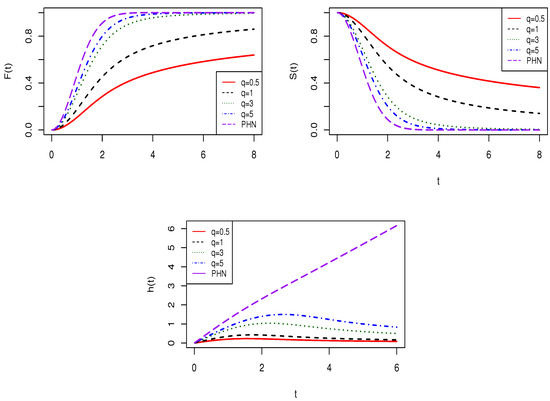
Figure 2. Plots of the cdf, survival function and hazard function for the SPHN $(1,2,q)$.

These plots suggest that:

(1)

For increasing values of q, the $SPHN(\sigma ,\alpha ,q)$ approaches the $PHN(\sigma ,\alpha )$ distribution (proven in Proposition 5).

(2)

For $\sigma$ and $\alpha$ fixed, these models are stochastically ordered with respect to q (proven in Section 2.4).

Proposition 3.

Let $T\sim SPHN(\sigma ,\alpha ,q)$. Then

1. 

For $0<\alpha \le 1$, the mode of T is at zero.

2. 

For $1<\alpha$, the mode of T can be obtained as the solution for $t>0$ of

$$g_X(t;\sigma ,\alpha )=(q+1)\frac{\alpha {\sigma }^q}{t^{q+1}}{M}_{\alpha ,q}\left(2\Phi \left(\frac{t}{\sigma }\right)-1\right),$$

(10)

where $\sigma >0$, $\alpha >0$, $q>0$, $M_{\alpha ,q}(·)$ was introduced in (8), and $g_X$ denotes the pdf of a $PHN(\sigma ,\alpha )$ model.

Proof. 

1. It follows from the fact that for $0<\alpha \le 1$, the pdf of T is a strictly decreasing function of t.

2. For $1<\alpha$, let us consider $\frac{d}{dt}{f}_T(t;\sigma ,\alpha ,q)=0$, i.e.,

$$\frac{d}{dt}\left(\frac{{\sigma }^q\alpha q}{t^{q+1}}{M}_{\alpha ,q}\left(2\Phi \left(\frac{t}{\sigma }\right)-1\right)\right)=0.$$

Equivalently,

$$\frac{d}{dt}\left(\frac{{\sigma }^q\alpha q}{t^{q+1}}\right)M_{\alpha ,q}\left(2\Phi \left(\frac{t}{\sigma }\right)-1\right)+\frac{{\sigma }^q\alpha q}{t^{q+1}}\frac{d}{dt}\left(M_{\alpha ,q}\left(2\Phi \left(\frac{t}{\sigma }\right)-1\right)\right)=0.$$

Thus,

$$\frac{{\sigma }^q\alpha q(-q-1)}{t^{q+2}}{M}_{\alpha ,q}\left(2\Phi \left(\frac{t}{\sigma }\right)-1\right)+\frac{2\alpha q}{\sigma t}\varphi \left(\frac{t}{\sigma }\right){\left(2\Phi \left(\frac{t}{\sigma }\right)-1\right)}^{\alpha -1}=0,$$

which is equivalent to (10). □

Remark 2.

(10) must be solved numerically.

Next, it is proven that the SPHN model can be expressed as a scale mixture of distributions.

Proposition 4.

Let $T|U=u\sim PHN(u^{-1/q}\sigma ,\alpha )$ and $U\sim U(0,1)$. Then, $T\sim SPHN(\sigma ,\alpha ,q)$.

Proof. 

Note that the marginal pdf of T can be obtained as

$$f_T(t;\sigma ,\alpha ,q)={\int }_0^1{f}_{T|U}\left(t\right|u)f_U\left(u\right)du={\int }_0^1\frac{2\alpha u^{1/q}}{\sigma }\varphi \left(\frac{t{u}^{1/q}}{\sigma }\right){\left(2\Phi \left(\frac{t{u}^{1/q}}{\sigma }\right)-1\right)}^{\alpha -1}du.$$

Making the change of variable $v=2\Phi \left(\frac{t{u}^{1/q}}{\sigma }\right)-1$, the proposed result is obtained. □

By applying the method proposed in Barranco-Chamorro et al. [15], the convergence in law of the $SPHN(\sigma ,\alpha ,q)$ model, as $q\to \infty$, to a $PHN(\sigma ,\alpha )$ distribution is next established. To highlight the fact that we are taking the limit for $q\to \infty$, the subindex q is used to refer to $T_q\sim SPHN(\sigma ,\alpha ,q)$.

Proposition 5.

Let $T_q\sim SPHN(\sigma ,\alpha ,q)$. If $q\to \infty$, then $T_q$ converges in distribution to $X\sim PHN(\sigma ,\alpha )$.

Proof. 

It is given in Appendix B. □

Note that the result given in Proposition 5 states that for large values of q, the $SPHN(\sigma ,\alpha ,q)$ model can be approached by a $PHN(\sigma ,\alpha )$ distribution.

2.2. Relationships among Distributions

In the following, we will see special cases that are associated with the SPHN distribution.

• According to Proposition 5, if $q\to \infty$ then $T\stackrel{d}{⟶}X$, where $X\sim PHN(\sigma ,\alpha )$. That is, the SPHN model contains the PHN model as a limit case.
• If $\alpha =1$, then $T=Y$ with $\sigma =\frac{1}{2}\beta$, where Y follows a slash half-normal (SHN) distribution introduced in Olmos et al. [9].
• If $q\to \infty$ and $\alpha =1$, then $T\stackrel{d}{⟶}M$, where M follows an $HN\left(\sigma \right)$ distribution.

These relationships among distributions are summarized in Figure 3.

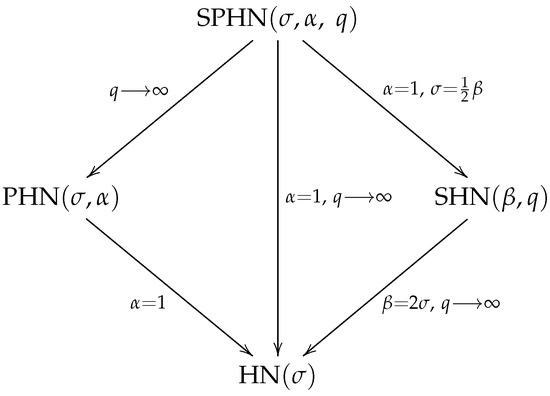
Figure 3. Relationships among distributions in the SPHN family.

2.3. Moments

The next proposition gives us the expresion of noncentral moments in the SPHN distribution. The expected value, variance, skewness and kurtosis coefficients follow in a straightforward way.

Proposition 6.

Let $T\sim SPHN(\sigma ,\alpha ,q)$. Then, for $r=1,2,\dots$ and $q>r$, the rth-non-central moment of T exists and is given by

$${\mu }_r=E\left(T^r\right)=\frac{q\alpha {\sigma }^r}{q-r}{\kappa }_r\left(\alpha \right),$$

(11)

where ${\kappa }_r={\kappa }_r\left(\alpha \right)={\int }_0^1{\left({\Phi }^{-1}\left(\frac{1+u}{2}\right)\right)}^r{u}^{\alpha -1}du.$

Proof. 

By using the stochastic representation for the SPHN distribution given in (6), we have that

$$\begin{array}{c}{\mu }_r=E\left(T^r\right)=E\left({\left(\frac{X}{Y^{\frac{1}{q}}}\right)}^r\right)=E\left(X^r{Y}^{-\frac{r}{q}}\right)=E\left(X^r\right)E\left(Y^{-\frac{r}{q}}\right).\end{array}$$

On the one hand, we have that $E\left(Y^{-\frac{r}{q}}\right)$ exists for $q>r$ and $E\left(Y^{-\frac{r}{q}}\right)=\frac{q}{q-r}.$ On the other hand, $E\left(X^r\right)=\alpha {\sigma }^r{\kappa }_r\left(\alpha \right)$ is the rth-moment of a $PHN(\sigma ,\alpha )$ model given in (2).

So, (11) is obtained. □

Remark 3.

Note that from Proposition 6, given $T\sim SPHN(\sigma ,\alpha ,q)$, for $r\ge q$, ${\mu }_r=E\left(T^r\right)$ is infinity.

From (2) and (11), the following relationship between the moments of SHPN and PHN models follows.

Corollary 3.

Let $T\sim SPHN(\sigma ,\alpha ,q)$ and $X\sim PHN(\sigma ,\alpha )$. Then

$$E\left(T^r\right)=\frac{q}{q-r}E\left(X^r\right),q>r.$$

(12)

Corollary 4.

Let $T\sim SPHN(\sigma ,\alpha ,q)$. Then

$$\begin{array}{ccc}\hfill E\left(T\right)& =& \frac{\sigma \alpha q}{q-1}{\kappa }_1,q>1,\hfill \end{array}$$

(13)

$$\begin{array}{ccc}\hfill Var\left(T\right)& =& \frac{{\sigma }^2\alpha q\left[{(q-1)}^2{\kappa }_2-\alpha q(q-2){\kappa }_1^2\right]}{{(q-1)}^2(q-2)},q>2,\hfill \end{array}$$

(14)

where ${\kappa }_r={\kappa }_r\left(\alpha \right)={\int }_0^1{\left({\Phi }^{-1}\left(\frac{1+u}{2}\right)\right)}^r{u}^{\alpha -1}du.$

For illustrative purposes, the expected value, variance and mode for different values of parameters in the SHPN model are given in Table 2. We observe that the expected value, variance and mode decrease as q increases for the the values of the parameters under consideration.

Table 2. Values of mean, variance and mode.

Parameters	Mean	Variance	Mode
$\sigma =1$, $\alpha =2$, $q=3$	1.692	2.045	1.066
$\sigma =1$, $\alpha =2$, $q=4$	1.505	1.010	1.033
$\sigma =1$, $\alpha =2$, $q=5$	1.410	0.738	1.009
$\sigma =1.5$, $\alpha =2$, $q=3$	2.539	4.601	1.599
$\sigma =1.5$, $\alpha =2$, $q=4$	2.257	2.272	1.549
$\sigma =1.5$, $\alpha =2$, $q=5$	2.116	1.661	1.514
$\sigma =2$, $\alpha =2$, $q=3$	3.385	8.180	2.131
$\sigma =2$, $\alpha =2$, $q=4$	3.009	4.039	2.065
$\sigma =2$, $\alpha =2$, $q=5$	2.821	2.953	2.019

Corollary 5.

Let $T\sim SPHN(\sigma ,\alpha ,q)$. Then, the skewness, $\sqrt{{\beta }_1}$, and kurtosis, ${\beta }_2$, coefficients are, for $q>3$,

$$\sqrt{{\beta }_1}=\frac{\sqrt{(q-2)}\left[{(q-1)}^3(q-2){\kappa }_3-3q\alpha {(q-1)}^2(q-3){\kappa }_1{\kappa }_2+2q^2{\alpha }^2(q-2)(q-3){\kappa }_1^3\right]}{\sqrt{\alpha q}(q-3){[{(q-1)}^2{\kappa }_2-\alpha q(q-2){\kappa }_1^2]}^{3/2}},$$

and for $q>4$,

$${\beta }_2=\frac{A}{\alpha q(q-3)(q-4){[{(q-1)}^2{\kappa }_2-\alpha q(q-2){\kappa }_1^2]}^2},$$

where $A={(q-1)}^2{(q-2)}^2[(q-1)(q-3){\kappa }_4-4\alpha q(q-4){\kappa }_1{\kappa }_3]+{\alpha }^2{q}^2(q-2)(q-3)(q-4)[6{(q-1)}^2{\kappa }_1^2{\kappa }_2-3\alpha q(q-2){\kappa }_1^4]$.

Remark 4.

The skewness and kurtosis coefficients were obtained by using

$$\sqrt{{\beta }_1}=\frac{{\mu }_3-3{\mu }_1{\mu }_2+2{\mu }_1^3}{{({\mu }_2-{\mu }_1^2)}^{\frac{3}{2}}},and{\beta }_2=\frac{{\mu }_4-4{\mu }_1{\mu }_3+6{\mu }_2{\mu }_1^2-3{\mu }_1^4}{{({\mu }_2-{\mu }_1^2)}^2}.$$

Figure 4 and Figure 5 provides plots for the skewness and kurtosis coefficients in the SPHN distribution. Both coefficients depend on $\alpha$ and q parameters. $\sqrt{{\beta }_1}$ and ${\beta }_2$ do not depend on $\sigma$, since $\sigma$ is a scale parameter.

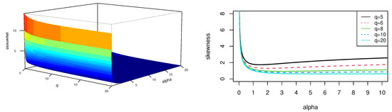
Figure 4. Plots of the skewness coefficient in the SPHN model.

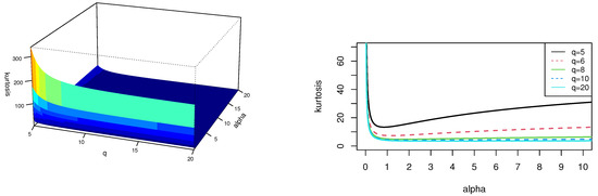
Figure 5. Plots of the kurtosis coefficient in the SPHN model.

2.4. Stochastic Ordering

Proposition 7.

Let $X\sim PHN(\sigma ,\alpha )$, $T_1\sim SPHN(\sigma ,\alpha ,q_1)$, and $T_2\sim SPHN(\sigma ,\alpha ,q_2)$ with $0<q_1<q_2$ (σ, $\alpha >0$ fixed). Then, X is stochastically smaller than $T_2$, $X{\le }_{st}{T}_2$, and $T_2$ is stochastically smaller than $T_1$, $T_2{\le }_{st}{T}_1$. So, as summary, we can write

$$X{\le }_{st}{T}_2{\le }_{st}{T}_1.$$

(15)

Proof. 

From Corollary 2, and the fact that $M_{\alpha ,q}(·)$, defined in (8), is a decreasing function of q, we can write the following relationship among the survival functions of X, $T_1$ and $T_2$

$$S_X(t;\sigma ,\alpha )\le S_{T_2}(t;\sigma ,\alpha ,q_2)\le S_{T_1}(t;\sigma ,\alpha ,q_1),\forall t.$$

It can be seen in [16] that this is the definition of stochastic order, and therefore, (15) follows. □

Corollary 6.

Let $X\sim PHN(\sigma ,\alpha )$, $T_1\sim SPHN(\sigma ,\alpha ,q_1)$, and $T_2\sim SPHN(\sigma ,\alpha ,q_2)$ with $1<q_1<q_2$ (σ, $\alpha >0$ fixed). Then

$$E\left(X\right)\le E\left(T_2\right)\le E\left(T_1\right).$$

(16)

Proof. 

Since for $q_i>1$, $E\left(T_i\right)$ exists $i=1,2$, then, it can be seen in [16] that from (15) follows (16). □

In addition, some relationships can be given for the order statistics of these distributions.

Proposition 8.

Let $X_1,\dots ,X_n$ be a random sample of $X\sim PHN(\sigma ,\alpha )$, and let us denote by $X_{\left(j\right)}$ the j-$th$ order statistic in this sample, $j=1,\dots ,n$. Similarly, let us consider $T_1^i,\dots ,T_n^i$ a random sample of $T_i\sim SPHN(\sigma ,\alpha ,q_i)$, $i=1,2,$ with $q_1<q_2$, and $T_{\left(j\right)}^i$ denotes the j-$th$ order statistic for the sample of $T_i$. Then, the j-$th$ order statistics are also stochastically ordered, explicitly,

$$X_{\left(j\right)}{\le }_{st}{T}_{\left(j\right)}^2{\le }_{st}{T}_{\left(j\right)}^1,j=1,\dots ,n.$$

(17)

Proof. 

It can be seen in [16] that this result is a consequence of (15). □

3. Inference

In this section, the estimation of parameters is carried out by applying moment and maximum likelihood (ML) methods. A simulation study is carried out in Section 4 to asses the performance of ML estimates when the sample size increases.

3.1. Moment Estimators

Let $T_1,T_2,\dots ,T_n$ be a random sample of $T\sim SPHN(\sigma ,\alpha ,q)$. From $E\left(T\right)=\overline{T}$ and (11), we can write

$$\sigma =\frac{(q-1)\overline{T}}{\alpha q{\kappa }_1}.$$

(18)

By using (11) again, and replacing the second and third population moments by the corresponding second and third sampling moments, the following equations are obtained

$$\begin{array}{ccc}\hfill \overline{T^2}\alpha q(q-2){\kappa }_1^2& =& {\overline{T}}^2{(q-1)}^2{\kappa }_2,\hfill \end{array}$$

(19)

$$\begin{array}{ccc}\hfill \overline{T^3}{\alpha }^2{q}^2(q-3){\kappa }_1^3& =& {\overline{T}}^3{(q-1)}^3{\kappa }_3.\hfill \end{array}$$

(20)

The system of equations generated by (19) and (20) be solved numerically: for instance, by using, $\mathtt{R}$ [17], leading to the moment estimators ${\widehat{\alpha }}_M$ and ${\widehat{q}}_M$. The moment estimator, ${\widehat{\sigma }}_M$, is obtained from Equation (18), by replacing $\alpha$ by ${\widehat{\alpha }}_M$ and q by ${\widehat{q}}_M$.

3.2. ML Estimators

In this subsection, the ML equations are introduced for the parameters $(\sigma ,\alpha ,q)$ on the SPHN model. Let $t_1,t_2,\dots ,t_n$ be a random sample from $T\sim SPHN(\sigma ,\alpha ,q)$. Then, the log-likelihood function can be expressed as

$$l(\sigma ,\alpha ,q)=nqlog\left(\sigma \right)+nlog\left(\alpha \right)+nlog\left(q\right)-(q+1)\sum _{i=1}^{n}log\left(t_i\right)+\sum _{i=1}^{n}log\left(M\left(v_i\right)\right),$$

(21)

where $v_i=2\Phi \left(\frac{t_i}{\sigma }\right)-1$ and $M\left(v_i\right)=M_{\alpha ,q}\left(v_i\right)$   $i=1,\dots ,n$.

The ML estimates are obtained by maximizing the equation given in (21). Taking the first derivative of the log-likelihood function with respect to each parameter, the following estimating equations are obtained, where we denote by $\mathit{\theta }=(\sigma ,\alpha ,q)$

$$\begin{array}{ccc}\hfill \frac{\partial l\left(\mathit{\theta }\right)}{\partial \sigma }& =& \frac{nq}{\sigma }+\sum _{i=1}^n\frac{M_1\left(v_i\right)}{M\left(v_i\right)}=0,\hfill \end{array}$$

(22)

$$\begin{array}{ccc}\hfill \frac{\partial l\left(\mathit{\theta }\right)}{\partial \alpha }& =& \frac{n}{\alpha }+\sum _{i=1}^n\frac{M_2\left(v_i\right)}{M\left(v_i\right)}=0,\hfill \end{array}$$

(23)

$$\begin{array}{ccc}\hfill \frac{\partial l\left(\mathit{\theta }\right)}{\partial q}& =& nlog\left(\sigma \right)+\frac{n}{q}-\sum _{i=1}^{n}log\left(t_i\right)+\sum _{i=1}^n\frac{M_3\left(v_i\right)}{M\left(v_i\right)}=0,\hfill \end{array}$$

(24)

where $M_1\left(v_i\right)=\frac{\partial M\left(v_i\right)}{\partial \sigma }$, $M_2\left(v_i\right)=\frac{\partial M\left(v_i\right)}{\partial \alpha }$ and $M_3\left(v_i\right)=\frac{\partial M\left(v_i\right)}{\partial q}$.

Equations (22)–(24) must be solved by using numerical procedures, such as the optim function in R software. Other maximization techniques could be applied, which directly maximize the log-likelihood function: for instance, the method proposed in McDonald [18].

Under regularity conditions, the asymptotic distribution of the MLEs $\widehat{\mathit{\theta }}=(\widehat{\sigma },\widehat{\alpha },\widehat{q})$ is a trivariate normal with mean vector $\mathit{\theta }$ and variance–covariance matrix that is the inverse of the Fisher information matrix, $I{\left(\mathit{\theta }\right)}^{-1}$. Usually, $I\left(\mathit{\theta }\right)$ is estimated by the observed information matrix $I\left(\widehat{\mathit{\theta }}\right)$ given by

$$I\left(\widehat{\mathit{\theta }}\right)={\left.\left(-\frac{{\partial }^{2}l\left(\mathit{\theta }\right)}{\partial \mathit{\theta }\partial {\mathit{\theta }}^T}\right)\right|}_{\mathit{\theta }=\widehat{\mathit{\theta }}}={\left.\left(\begin{array}{ccc}{I}_{\sigma ,\sigma }& I_{\sigma ,\alpha }& I_{\sigma ,q}\\ I_{\alpha ,\sigma ,}& I_{\alpha ,\alpha }& I_{\alpha ,q}\\ I_{q,\sigma }& I_{q,\alpha }& I_{q,q}\end{array}\right)\right|}_{\mathit{\theta }=\widehat{\mathit{\theta }}},$$

whose elements are

$$\begin{array}{ccc}\hfill I_{\sigma ,\sigma }& =& -\frac{{\partial }^{2}l\left(\mathit{\theta }\right)}{\partial {\sigma }^2}=\frac{nq}{{\sigma }^2}-\sum _{i=1}^n\frac{M_{1,1}\left(v_i\right)M\left(v_i\right)-M_1^2\left(v_i\right)}{M^2\left(v_i\right)},\hfill \\ \hfill I_{\sigma ,\alpha }& =& -\frac{{\partial }^{2}l\left(\mathit{\theta }\right)}{\partial \sigma \partial \alpha }=-\sum _{i=1}^n\frac{M_{1,2}\left(v_i\right)M\left(v_i\right)-M_1\left(v_i\right)M_2\left(v_i\right)}{M^2\left(v_i\right)}\hfill \\ \hfill I_{\sigma ,q}& =& -\frac{{\partial }^{2}l\left(\mathit{\theta }\right)}{\partial \sigma \partial q}=-\frac{n}{\sigma }-\sum _{i=1}^n\frac{M_{1,3}\left(v_i\right)M\left(v_i\right)-M_3\left(v_i\right)M_1\left(v_i\right)}{M^2\left(v_i\right)},\hfill \\ \hfill I_{\alpha ,\alpha }& =& -\frac{{\partial }^{2}l\left(\mathit{\theta }\right)}{\partial {\alpha }^2}=\frac{n}{{\alpha }^2}-\sum _{i=1}^n\frac{M_{2,2}\left(v_i\right)M\left(v_i\right)-M_2^2\left(v_i\right)}{M^2\left(v_i\right)},\hfill \\ \hfill I_{\alpha ,q}& =& -\frac{{\partial }^{2}l\left(\mathit{\theta }\right)}{\partial \alpha \partial q}=-\sum _{i=1}^n\frac{M_{2,3}\left(v_i\right)M\left(v_i\right)-M_3\left(v_i\right)M_2\left(v_i\right)}{M^2\left(v_i\right)}\hfill \\ \hfill I_{q,q}& =& -\frac{{\partial }^{2}l\left(\mathit{\theta }\right)}{\partial q^2}=\frac{n}{q^2}-\sum _{i=1}^n\frac{M_{3,3}\left(v_i\right)M\left(v_i\right)-M_3^2\left(v_i\right)}{M^2\left(v_i\right)},\hfill \end{array}$$

with $M_{j,k}\left(v_i\right)=\frac{{\partial }^{2}M\left(v_i\right)}{\partial {\mathit{\theta }}_j\partial {\mathit{\theta }}_k}$ and $\mathit{\theta }=(\sigma ,\alpha ,q)$.

From the asymptotic normality of MLEs, approximate confidence intervals can be proposed for ${\theta }_i$. So, an Asymptotic Confidence Interval (ACI) at confidence level $1-\gamma$, $0<\gamma <1$, for ${\theta }_i=\sigma$, $\alpha$, q is

$$ACI({\theta }_i,1-\gamma )={\widehat{\theta }}_i\pm z_{1-\gamma /2}s.e.\left({\widehat{\theta }}_i\right),\mathrm{where}{\widehat{\theta }}_i=\{\widehat{\sigma },\widehat{\alpha },\widehat{q}\},$$

the standard error of ${\widehat{\theta }}_i$, $s.e.\left({\widehat{\theta }}_i\right)$, is the squared root of the $i\mathrm{th}$ diagonal element of $I{\left(\widehat{\mathit{\theta }}\right)}^{-1}$, and $z_{1-\gamma /2}$ denotes the quantile of order $1-\gamma /2$ in the $N(0,1)$ distribution.

4. Simulation Study

In this section, a simulation study is conducted aiming to investigate ML estimation performance for parameters $\sigma$, $\alpha$ and q in the SPHN model. Specifically, 1000 random samples of sizes $n=$ 50, 100 and 200 were generated under the SPHN model by using the algorithm given below. A summary of the results obtained in this study are depicted in Table 3. The empirical means correspond to the means of the estimated parameters over the 1000 simulated samples. The SE given in Table 3 is the average of the standard errors obtained in every simulation, $s.e.\left({\widehat{\theta }}_i\right)$, which were calculated as the square root of the corresponding diagonal element in the inverse of the observed information matrix. Moreover, Asymptotic Confidence Intervals (ACIs) at confidence level $1-\gamma$, $0<\gamma <1$, have been built based on the asymptotic normality of MLEs. Specifically,

$$ACI({\theta }_i,1-\gamma )=\left({\widehat{\theta }}_i-z_{1-\gamma /2}s.e.\left({\widehat{\theta }}_i\right),{\widehat{\theta }}_i+z_{1-\gamma /2}s.e.\left({\widehat{\theta }}_i\right)\right),\mathrm{with}{\widehat{\theta }}_i=\{\widehat{\sigma },\widehat{\alpha },\widehat{q}\}.$$

(25)

Table 3. Empirical means and SE for the ML estimates of $\sigma$, $\alpha$ and q.

True Value			$\mathit{n}=50$			$\mathit{n}=100$			$\mathit{n}=200$
($\mathbf{\sigma }$,$\mathbf{\alpha }$,$\mathit{q}$)		Means (SE)	RMSE	CP	Means (SE)	RMSE	CP	Means (SD)	RMSE	CP
(1, 1, $0.2$)	$\widehat{\sigma }$	1.2756 (1.2458)	0.8082	0.9190	1.1000 (0.4882)	0.6382	0.9480	1.0492 (0.3259)	0.3963	0.9680
	$\widehat{\alpha }$	1.4480 (1.2375)	2.1143	0.9190	1.2444 (0.5203)	0.9947	0.9350	1.0743 (0.2300)	0.3050	0.9550
	$\widehat{q}$	0.2095 (0.0342)	0.0363	0.9290	0.2035 (0.0233)	0.0238	0.9350	0.2026 (0.0163)	0.0161	0.9650
(1, 1, $0.5$)	$\widehat{\sigma }$	1.0902 (0.4679)	0.6130	0.9310	1.0384 (0.3114)	0.3490	0.9520	1.0220 (0.2167)	0.2239	0.9660
	$\widehat{\alpha }$	1.2433 (0.5597)	1.2440	0.9060	1.0937 (0.2760)	0.5732	0.9560	1.0327 (0.1511)	0.1552	0.9710
	$\widehat{q}$	0.5307 (0.1046)	0.1176	0.9360	0.5167 (0.0706)	0.0763	0.9520	0.5080 (0.0485)	0.0505	0.9780
(1, 1, 1)	$\widehat{\sigma }$	1.0615 (0.3547)	0.4391	0.9050	1.0272 (0.2385)	0.2564	0.9340	1.0135 (0.1668)	0.1758	0.9680
	$\widehat{\alpha }$	1.1044 (0.2987)	0.4388	0.9140	1.0463 (0.1797)	0.1978	0.9330	1.0225 (0.1217)	0.1254	0.9680
	$\widehat{q}$	1.1134 (0.3335)	0.4455	0.9160	1.0544 (0.1866)	0.2101	0.9230	1.0229 (0.1248)	0.1352	0.9650
(1, 1, 2)	$\widehat{\sigma }$	1.0303 (0.3110)	0.3048	0.9070	1.0368 (0.2125)	0.2363	0.9330	1.0167 (0.1405)	0.1398	0.9590
	$\widehat{\alpha }$	1.0761 (0.2339)	0.2654	0.9370	1.0280 (0.1521)	0.1601	0.9590	1.0117 (0.1039)	0.1014	0.9780
	$\widehat{q}$	2.9366 (6.2097)	5.2450	0.9120	2.5031 (1.7373)	2.3456	0.9470	2.1185 (0.4051)	0.4622	0.9720
(1, 1, 3)	$\widehat{\sigma }$	1.0049 (0.3290)	0.2750	0.9360	1.0244 (0.2111)	0.1911	0.9560	1.0211 (0.1393)	0.1395	0.9700
	$\widehat{\alpha }$	1.0848 (0.2257)	0.2514	0.9120	1.0330 (0.1454)	0.1493	0.9350	1.0111 (0.0986)	0.0983	0.9630
	$\widehat{q}$	6.0879 (31.8647)	15.6052	0.8190	4.2446 (7.8499)	6.8776	0.8420	3.6100 (3.3989)	3.2592	0.8650
(1, 2, $0.2$)	$\widehat{\sigma }$	1.3295 (0.7451)	1.7989	0.9590	1.0159 (0.4083)	0.4906	0.9690	1.0154 (0.2835)	0.3181	0.9770
	$\widehat{\alpha }$	4.8723 (10.4037)	16.7010	0.9010	5.4312 (8.4096)	25.9159	0.9170	2.5311 (1.3470)	2.9316	0.9410
	$\widehat{q}$	0.2098 (0.0327)	0.0352	0.9370	0.2030 (0.0221)	0.0226	0.9540	0.2022 (0.0156)	0.0152	0.9640
(1, 2, $0.5$)	$\widehat{\sigma }$	1.0344 (0.4007)	0.4556	0.9390	1.0080 (0.2698)	0.3167	0.9580	1.0060 (0.1860)	0.1902	0.9790
	$\widehat{\alpha }$	4.7341 (8.3355)	26.6807	0.9000	3.0202 (2.6570)	17.3013	0.9590	2.1518 (0.4745)	0.5434	0.9750
	$\widehat{q}$	0.5245 (0.0934)	0.0991	0.9280	0.5126 (0.0637)	0.0688	0.9580	0.5059 (0.0440)	0.0455	0.9720
(1, 2, 1)	$\widehat{\sigma }$	1.0362 (0.2978)	0.3843	0.9110	1.0172 (0.2007)	0.2185	0.9290	1.0058 (0.1402)	0.1464	0.9550
	$\widehat{\alpha }$	2.6554 (1.5279)	4.1685	0.9440	2.1698 (0.52600)	0.6510	0.9690	2.0801 (0.3386)	0.3638	0.9710
	$\widehat{q}$	1.0886 (0.3429)	0.5496	0.9170	1.0382 (0.1560)	0.1693	0.9300	1.0156 (0.1060)	0.1133	0.9600
(1, 2, 2)	$\widehat{\sigma }$	1.0469 (0.2610)	0.2788	0.9330	1.0147 (0.1678)	0.1825	0.9570	1.0081 (0.1145)	0.1119	0.9660
	$\widehat{\alpha }$	2.2165 (0.6503)	0.8276	0.9450	2.1070 (0.4123)	0.4585	0.9520	2.0405 (0.2687)	0.2683	0.9610
	$\widehat{q}$	2.7106 (8.2183)	4.6692	0.9450	2.2108 (0.6296)	0.9698	0.8690	2.0656 (0.3028)	0.3293	0.9790
(1, 2, 3)	$\widehat{\sigma }$	1.0079 (0.2491)	0.2356	0.9240	1.0236 (0.1631)	0.1693	0.9370	1.0115 (0.1094)	0.1131	0.9540
	$\widehat{\alpha }$	2.2321 (0.6068)	0.7837	0.9300	2.0868 (0.3648)	0.3965	0.9560	2.0342 (0.2470)	0.2540	0.9650
	$\widehat{q}$	4.4271 (21.5189)	6.5850	0.9330	3.7860 (5.0595)	4.0973	0.9500	3.2516 (0.7341)	0.8807	0.9760
(5, 1, $0.2$)	$\widehat{\sigma }$	7.1646 (4.7763)	8.8383	0.9150	5.6108 (2.3005)	3.1957	0.9310	5.3230 (1.5285)	1.9831	0.9640
	$\widehat{\alpha }$	1.5457 (2.5030)	4.8049	0.9340	1.1815 (0.4875)	0.7967	0.9480	1.0602 (0.2235)	0.2538	0.9710
	$\widehat{q}$	0.2121 (0.0348)	0.0379	0.9400	0.2048 (0.0233)	0.0242	0.9540	0.2032 (0.0164)	0.0165	0.9640
(5, 1, $0.5$)	$\widehat{\sigma }$	5.7373 (2.4456)	3.5837	0.8340	5.2045 (1.5400)	1.7220	0.8820	5.1184 (1.0609)	1.1176	0.9130
	$\widehat{\alpha }$	1.1659 (0.4008)	0.5596	0.9230	1.0860 (0.2721)	0.5568	0.9350	1.0320 (0.1502)	0.1582	0.9690
	$\widehat{q}$	0.5406 (0.1080)	0.1230	0.9250	0.5172 (0.0706)	0.0746	0.9460	0.5076 (0.0485)	0.0493	0.9760
(5, 1, 1)	$\widehat{\sigma }$	5.5348 (2.3423)	1.8272	0.9130	5.1725 (1.1825)	1.3342	0.9300	5.0665 (0.8744)	0.8161	0.9640
	$\widehat{\alpha }$	1.0863 (0.2764)	0.3496	0.9130	1.0438 ( 0.1991)	0.1778	0.9320	1.0202 (0.1204)	0.1251	0.9680
	$\widehat{q}$	1.1710 (0.9094)	1.1789	0.9120	1.0572 (0.2180)	0.1868	0.9420	1.0216 (0.1349)	0.1238	0.9670
(5, 1, 2)	$\widehat{\sigma }$	5.1390 (1.5468)	1.5353	0.9130	5.2000 (1.0311)	1.1426	0.9350	5.0772 (0.6857)	0.6987	0.9680
	$\widehat{\alpha }$	1.0858 (0.2367)	0.2748	0.9180	1.0239 (0.1503)	0.1566	0.9520	1.0120 (0.1034)	0.0998	0.9730
	$\widehat{q}$	3.1212 (11.2902)	5.8760	0.9320	2.4613 (1.2155)	2.0554	0.9450	2.1162 (0.4021)	0.4727	0.9670
(5, 1, 3)	$\widehat{\sigma }$	5.0359 (1.6298)	1.3186	0.9200	5.0808 (1.0229)	0.9645	0.9490	5.1051 (0.6823)	0.6916	0.9680
	$\widehat{\alpha }$	1.0719 (0.2196)	0.2480	0.9290	1.0372 (0.1454)	0.1524	0.9410	1.0115 (0.0983)	0.1003	0.9600
	$\widehat{q}$	5.5128 (40.7540)	10.3607	0.8670	4.0842 (10.7407)	5.8639	0.8910	3.5737 (1.6583)	3.5863	0.9080
(5, 2, $0.2$)	$\widehat{\sigma }$	6.2208 (3.4545)	4.2936	0.9240	5.2606 (2.1131)	2.2751	0.9450	5.1968 (1.4418)	1.6041	0.9640
	$\widehat{\alpha }$	5.1805 (25.4483)	23.6679	0.8940	3.8097 (7.1766)	10.5513	0.9110	2.3044 (0.8466)	1.0814	0.9200
	$\widehat{q}$	0.2171 (0.0340)	0.0371	0.9070	0.2062 (0.0225)	0.0226	0.9420	0.2018 (0.0155)	0.0151	0.9660
(5, 2, $0.5$)	$\widehat{\sigma }$	5.3204 (2.0113)	2.6829	0.9350	5.1098 (1.3326)	1.4756	0.9420	5.0095 (0.9002)	0.9582	0.9620
	$\widehat{\alpha }$	3.1852 (2.6410)	4.8063	0.9010	2.4125 (0.9534)	2.1373	0.9200	2.1544 (0.4681)	0.5838	0.9390
	$\widehat{q}$	0.5367 (0.0961)	0.1081	0.9480	0.5139 (0.0636)	0.0677	0.9650	0.5038 (0.0435)	0.0458	0.9780
(5, 2, 1)	$\widehat{\sigma }$	5.1151 (1.4670)	1.8693	0.9100	5.0798 (0.9838)	1.0709	0.9220	5.0359 (0.6745)	0.7345	0.9330
	$\widehat{\alpha }$	3.6045 (3.4441)	23.5407	0.8500	2.1829 (0.5345)	0.9166	0.8980	2.0815 ( 0.3328)	0.3933	0.9200
	$\widehat{q}$	1.1051 (0.5248)	0.8640	0.9390	1.0358 (0.1548)	0.1665	0.9570	1.0176 (0.1054)	0.1129	0.9720
(5, 2, 2)	$\widehat{\sigma }$	5.1574 (1.2498)	1.4238	0.9110	5.0913 (0.8157)	0.9276	0.8900	5.0464 (0.5606)	0.5956	0.9650
	$\widehat{\alpha }$	2.3183(0.7369)	1.2030	0.9490	2.1076 (0.4006)	0.4665	0.9530	2.0411 (0.2661)	0.2847	0.9600
	$\widehat{q}$	2.7879 (3.6209)	7.7982	0.9260	2.1672 (0.5127)	0.6408	0.9490	2.0771 (0.3078)	0.3513	0.9690
(5, 2, 3)	$\widehat{\sigma }$	5.1098 (1.2615)	1.2178	0.9100	5.1094 (0.8084)	0.8635	0.9310	5.0502 (0.5223)	0.5619	0.9550
	$\widehat{\alpha }$	2.2587 (0.6545)	1.0586	0.9250	2.0858 (0.3623)	0.4156	0.9490	2.0386 (0.2428)	0.2554	0.9630
	$\widehat{q}$	4.7063 (20.0928)	7.5044	0.9340	3.8496 (4.7614)	4.6096	0.9600	3.2650 (0.7597)	0.9814	0.9750
(5, 4, $0.2$)	$\widehat{\sigma }$	5.9042 (3.2053)	3.9180	0.9050	5.1234 (1.9895)	2.0869	0.9320	4.9130 (1.3224)	1.3365	0.9520
	$\widehat{\alpha }$	15.5998 (98.4168)	36.5604	0.7830	12.6370 (28.5041)	39.3718	0.7860	7.6859 (8.6139)	20.8462	0.8180
	$\widehat{q}$	0.2205 (0.0336)	0.0364	0.9150	0.2090 (0.0223)	0.0222	0.9360	0.2029 ( 0.0152)	0.0153	0.9440
(5, 4, $0.5$)	$\widehat{\sigma }$	5.1084 (1.8148)	1.9934	0.9210	5.0839 (1.2629)	1.3986	0.9420	5.0012 (0.8331)	0.9553	0.8970
	$\widehat{\alpha }$	13.7575 (27.8922)	47.6750	0.779	6.9460 (6.5967)	16.5931	0.8210	4.8960 (2.0477)	4.0452	0.8420
	$\widehat{q}$	0.5386 (0.0903)	0.0973	0.9210	0.5153 (0.0604)	0.0646	0.9450	0.5083 (0.0416)	0.0443	0.9640
(5, 4, 1)	$\widehat{\sigma }$	4.9761 ( 1.3131)	1.4340	0.9590	4.9748 (0.8876)	0.9616	0.9650	4.9689 (0.5988)	0.6400	0.9700
	$\widehat{\alpha }$	7.6639 (10.0667)	23.3789	0.8220	4.8691 (1.8710)	3.7083	0.8490	4.3453 (1.0154)	1.2519	0.8790
	$\widehat{q}$	1.0477 (0.2055)	0.2238	0.9370	1.0319 (0.1391)	0.1492	0.9400	1.0110 (0.0946)	0.0950	0.9600
(5, 4, 2)	$\widehat{\sigma }$	5.0894 (1.0537)	1.2673	0.9250	5.0116 (0.6943)	0.7811	0.9630	5.0327 (0.4963)	0.5229	0.9710
	$\widehat{\alpha }$	5.4842 (2.5477)	6.1704	0.9280	4.4710 (1.1923)	1.6281	0.9460	4.1662 (0.7346)	0.8332	0.9640
	$\widehat{q}$	2.4047 ( 1.2242)	3.0378	0.9590	2.1001 (0.3816)	0.4388	0.9620	2.0613 (0.2596)	0.2781	0.9740
(5, 4, 3)	$\widehat{\sigma }$	5.0853 (1.0467)	1.0945	0.9350	5.0768 (0.7025)	0.7645	0.9460	5.0166 (0.4485)	0.4817	0.9620
	$\widehat{\alpha }$	4.8945 (1.8456)	3.0342	0.9250	4.3010 (1.0213)	1.3791	0.9480	4.1370 (0.6541)	0.7266	0.9680
	$\widehat{q}$	4.1080 (9.3733)	4.9578	0.9060	3.5935 (9.7476)	3.3672	0.9100	3.1361 (0.5106)	0.5840	0.9220

The level confidence is $1-\gamma =0.95$. To asses the performance of these summaries, the empirical covarage probability (CP) of (25) has been included in Table 3. That is the proportion of ACIs that contain the true value of the parameter.

In Table 3, RMSE denotes the square root of the empirical mean squared error: for instance, for $\widehat{\alpha }$, it is calculated as

$$RMSE\left(\widehat{\alpha }\right)=\sqrt{\frac{1}{n}\sum _{i=1}^n{({\widehat{\alpha }}_i-\alpha )}^2},$$

and so on.

Next, the algorithm used to generate samples from $T\sim SPHN(\sigma ,\alpha ,q)$ is introduced. The Algorithm 1 is based on (6) and the inversion of the cdf given in (1).

Algorithm 1: for generate samples from $T\sim SPHN\left(\sigma ,\alpha ,q\right)$.

1: Simulate $W\sim U(0,1)$. 2: Compute $X=\sigma {\Phi }^{-1}\left(\frac{1+W^{1/\alpha }}{2}\right)$. 3: Simulate $Y\sim U(0,1)$. 4: Compute $T=\frac{X}{Y^{\frac{1}{q}}}$.

As conclusions of this simulation study, we highlight that as the sample size increases, estimates become closer to the true parameter values. These results suggest that the estimated standard errors and RMSE become smaller as sample size increases: that is, the proposed estimators are consistent. As for the ACI, the results are satisfactory. We highlight that their empirical CP approaches to the nominal 0.95 confidence level as n increases.

Following reviewers’ recommendations, similar plots to the ones proposed in [19] have been carried out to illustrate the results in Table 3. So, the empirical coverage probabilities obtained for the asymptotic confidence intervals at 95% for $\sigma$, $\alpha$ and q for the sample sizes $n=50,100,200$ have been plotted in Figure 6. The columns correspond to the cases $(\sigma =1,\alpha =1,q)$, $(\sigma =5,\alpha =2,q)$ and $(\sigma =5,\alpha =4,q)$ in Table 3 and the panels by rows to $q=\{0.2,0.5,1,2,3\}$. It can be appreciated there that, in all cases, the empirical coverage probability approaches the confidence level 0.95 as the sample size increases. This plot also suggests that the approximate confidence intervals for q and $\sigma$ perform better than those for $\alpha$.

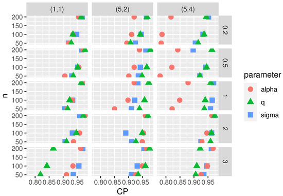
Figure 6. Empirical CP for the ACI ($n=50,100,200$) in the SPHN model $(\sigma =1,\alpha =1,q)=SHN(1,q)$, $(\sigma =5,\alpha =2,q)$, $(\sigma =5,\alpha =4,q)$ with $q=\{0.2,0.5,1,2,3\}$. In all panels, results for $\alpha$ (red point), q (green triangle), and $\sigma$ (blue square).

5. Applications

In this section, two real data sets with high kurtosis levels are considered. In these data sets, the PHN, GHN, Slash Power Maxwell (SPM) introduced in Segovia et al. [12], SGHN introduced in Olmos et al. [10] and SPHN distributions are considered. Details about these models can be seen in Appendix C.

The parameters are estimated by ML. The Akaike Information Criterion (AIC) and Bayesian Information Criterion (BIC), histograms and Q-Q plots are considered to compare these models.

5.1. Application 1

Let us consider the data set of kevlar 49/epoxy, which corresponds to fatigue fracture to constant pressure at the 90% stress level until the fail happened. This data set has been previously analyzed by Andrews and Herzberg [20], Barlow et al. [21] and Olmos et al. [9,10] among others. The data set consists of 101 observations with the presence of outliers. Explicitly, in Table 4:

Table 4. Data set of kevlar 49/epoxy.

0.01	0.01	0.02	0.02	0.02	0.03	0.03	0.04	0.05	0.06	0.07	0.07	0.08	0.09	0.09
0.10	0.10	0.11	0.11	0.12	0.13	0.18	0.19	0.20	0.23	0.24	0.24	0.29	0.34	0.35
0.36	0.38	0.40	0.42	0.43	0.52	0.54	0.56	0.60	0.60	0.63	0.65	0.67	0.68	0.72
0.72	0.72	0.73	0.79	0.79	0.80	0.80	0.83	0.85	0.90	0.92	0.95	0.99	1.00	1.01
1.02	1.03	1.05	1.10	1.10	1.11	1.15	1.18	1.20	1.29	1.31	1.33	1.34	1.40	1.43
1.45	1.50	1.51	1.52	1.53	1.54	1.54	1.55	1.58	1.6	1.63	1.64	1.80	1.80	1.81
2.02	2.05	2.14	2.17	2.33	3.03	3.03	3.34	4.20	4.69	7.89

In Table 5, the descriptive analysis is provided. We can see that this data set exhibits a high sample kurtosis coefficient of $16.709$, so it is interesting to see what can our model do here.

Table 5. Descriptive analysis for fatigue fracture data.

Mean	S.D.	Median	Range	Min.	Max.	Skewness	Kurtosis
1.025	1.119	0.800	7.88	0.010	7.890	3.002	16.709

For the SPHN model, the moment estimates are ${\widehat{\sigma }}_M=0.384$, ${\widehat{\alpha }}_M=3.653$ and ${\widehat{q}}_M=2.140$. These estimates are used as starting values to get the ML estimates by using numerical methods.

Table 6 shows the estimated parameters for each model under consideration. If we apply the AIC and BIC criteria, then the SPHN distribution must be preferred over the GHN, PHN, SPM and SGHN distributions, since its AIC and BIC are the smallest ones.

Table 6. Estimated values, standard errors (SE) in parentheses and criteria.

Distribution	ML Estimates (s.e.)			AIC	BIC
LogNormal	$\widehat{\mu }$ = 0.336 (0.002)	$\widehat{\sigma }$ = 1.844 (0.017)		230.62	240.47
GHN	$\widehat{\sigma }$ = 1.224 (0.017)	$\widehat{\alpha }$ = 0.711 (0.003)		210.67	215.90
PHN	$\widehat{\sigma }$ = 0.641 (0.005)	$\widehat{\alpha }$ = 1.821 (0.033)		217.24	222.47
SPM	$\widehat{\alpha }$ = 1.753 (0.008)	$\widehat{\beta }$ = 0.362 (8.41 $\times {10}^{-4}$)	$\widehat{q}$ = 10.012 (0.004)	213.68	221.47
SGHN	$\widehat{\sigma }$ = 0.835 (0.019)	$\widehat{\alpha }$ = 0.823 (0.007)	$\widehat{q}$ = 3.009 (1.235)	208.67	216.51
SPHN	$\widehat{\sigma }$ = 0.962 (0.031)	$\widehat{\alpha }$ = 0.760 (0.009)	$\widehat{q}$ = 2.822 (0.828)	207.43	215.28

Figure 7 shows the histograms for the fatigue fracture data set, along with the fitted distributions by using ML estimates in SPHN, GHN and SGHN models. The QQ-plot is also included to asses the good fit provided by the SPHN model to this data set.

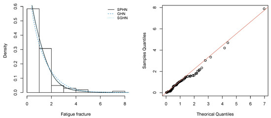
Figure 7. Left panel: Histograms of the fatigue fracture data fitted with the GHN, SGHN and SPHN distributions. Right panel: QQ plot for the SPHN distribution.

5.2. Application 2

Here, the data set previously analyzed by Gómez and Bolfarine [11] is considered. This data set corresponds to 72 survival times of guinea pigs injected with different doses of tubercle bacilli, which are in Table 7.

Table 7. Data set of survival times of guinea pigs.

12	15	22	24	24	32	32	33	34	38	38	43
44	48	52	53	54	54	55	56	57	58	58	59
60	60	60	60	61	62	63	65	65	67	68	70
70	72	73	75	76	76	81	83	84	85	87	91
95	96	98	99	109	110	121	127	129	131	143	146
146	175	175	211	233	258	258	263	297	341	341	376

The moment estimates for the parameters in the SPHN model are: ${\widehat{\sigma }}_M=41.681$, ${\widehat{\alpha }}_M=3.185$ and ${\widehat{q}}_M=2.304$. Again, these estimates are used as initial values to get the ML estimates by using numerical methods.

In Table 8, the descriptive analysis is given. We have that the sample kurtosis coefficient is $5.61$, so it is also interesting to see if the SPHN distribution can provide a good fit to this data set.

Table 8. Descriptive analysis for the survival times of guinea pigs.

Mean	S.D.	Median	Range	Min.	Max.	Skewness	Kurtosis
99.82	81.12	70.00	364	12.00	376.00	1.80	5.61

Table 9 shows the estimated parameters for each distribution. If we apply the statistical information criteria then, in all cases, both criteria choose the SPHN model over the GHN, PHN, SPM and SGHN distributions.

Table 9. Estimated values, SE and information criteria.

Distribution	ML Estimates (s.e.)			AIC	BIC
LogNormal	$\widehat{\mu }$ = 4.344 (0.007)	$\widehat{\sigma }$ = 0.710 (0.004)		788.67	793.22
GHN	$\widehat{\sigma }$ = 129.238 (141.55)	$\widehat{\alpha }$ = 1.016 (0.008)		807.29	812.03
PHN	$\widehat{\sigma }$ = 1.254 (0.035)	$\widehat{\alpha }$ = 117.343 (124.50)		805.24	807.48
SPM	$\widehat{\alpha }$ = 0.003 (5.29 $\times {10}^{-7}$)	$\widehat{\beta }$ = 0.783 (1.50 $\times {10}^{-4}$)	$\widehat{q}$ = 1.578 (0.009)	788.98	795.81
SGHN	$\widehat{\sigma }$ = 54.156 (1.138)	$\widehat{\alpha }$ = 2.594 (2.326 $\times {10}^{-7}$)	$\widehat{q}$ = 1.663 (0.003)	785.56	792.39
SPHN	$\widehat{\sigma }$ = 36.015 (0.022)	$\widehat{\alpha }$ = 3.216 (0.226)	$\widehat{q}$ = 1.799 (0.017)	785.04	791.87

Figure 8 shows the histograms for the guinea pigs survival time data along with the fitted distributions: SPHN, LogNormal, and SGHN, whose parameters were estimated by ML. The QQ-plot is also included for the proposed SPHN model, which provides the best fit to this data set.

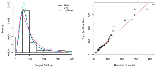
Figure 8. Left panel: Histograms of the survival times of guinea pigs data fitted by the LogNormal, SGHN and SPHN distributions. Right panel: QQ-plot of the SPHN distribution.

6. Conclusions

This paper introduces the SPHN distribution, which is built from the PHN distribution by using the slash methodology proposed in (6). In this way, a model with higher kurtosis than the PHN is obtained. The SPHN is a three-parameter model whose right tail is heavier for smaller values of the kurtosis parameter q. Relevant results of interest in reliability are discussed, such as cdf, survival, hazard rate function and stochastic orderings. The convergence in distribution to the PHN model is studied when the parameter of kurtosis q increases, along with the relationships with the PHN, SHN and HN models. All these relationships are summarized in Figure 3 and enhance the interest of our model. It is shown that the SPHN can be expressed of a scale mixture of a PHN and a uniform distribution. This property allows us to propose an algorithm to generate random values of the SPHN model. The unknown parameters in the model are estimated via ML. A simulation study is given where the good properties of ML estimators can be seen. As applications, two real data sets are considered with moderate and high kurtosis. These are Applications 2 and 1, respectively. Several common models are considered as competitors of SPHN. By applying information criteria (AIC and BIC), it is shown that our proposal provides the best fit to these data sets. Due to this fact, it is of interest to spread out the use and applications of this model.

Appendix A.1. SPHN for 0 < α < 1

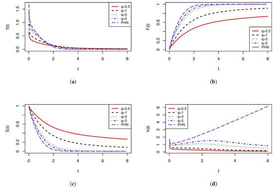
Figure A1. SPHN $(1,\alpha =0.8,q)$ for different values of q. In all panels, $q=0.5$ (red), $q=1$ (black), $q=3$ (green), $q=5$ (blue), and $q=\infty$ (purple). (a) pdf of SPHN $(1,\alpha =0.8,q)$. (b) cdf of SPHN $(1,\alpha =0.8,q)$. (c) Survival function of SPHN $(1,\alpha =0.8,q)$. (d) hazard rate function of SPHN $(1,\alpha =0.8,q)$.

Appendix A.2. SPHN for α = 1, Which Corresponds to the SHN Model

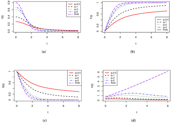
Figure A2. SPHN $(1,\alpha =1,q)=SHN(1,q)$ for different values of q. In all panels, $q=0.5$ (red), $q=1$ (black), $q=3$ (green), $q=5$ (blue), and $q=\infty$ (purple). (a) pdf of SPHN $(1,\alpha =1,q)$. (b) cdf of SPHN $(1,\alpha =1,q)$. (c) Survival function of SPHN $(1,\alpha =1,q)$. (d) hazard rate function of SPHN $(1,\alpha =1,q)$.

References

- Johnson, N.L.; Kotz, S.; Balakrishnan, N. Continuous Univariate Distributions, 2nd ed.; Wiley: New York, NY, USA, 1994; Volume 1. [Google Scholar]
- Rogers, W.H.; Tukey, J.W. Understanding some long-tailed symmetrical distributions. Stat. Neerl. 1972, 26, 211–226. [Google Scholar] [CrossRef]
- Mosteller, F.; Tukey, J.W. Data Analysis and Regression; A Second Course in Statistics; Addison-Wesley: Reading, MA, USA, 1977. [Google Scholar]
- Pewsey, A. Large-sample inference for the general half-normal distribution. Commun. Stat. Theory Methods 2002, 31, 1045–1054. [Google Scholar] [CrossRef]
- Pewsey, A. Improved likelihood based inference for the general half-normal distribution. Commun. Stat. Theory Methods 2004, 33, 197–204. [Google Scholar] [CrossRef]
- Wiper, M.P.; Girón, F.J.; Pewsey, A. Objective Bayesian inference for the half-normal and half-t distributions. Commun. Stat. Theory Methods 2008, 37, 3165–3185. [Google Scholar] [CrossRef]
- Cooray, K.; Ananda, M.M.A. A Generalization of the Half-Normal Distribution with Applications to Lifetime Data. Commun. Stat. Theory Methods 2008, 37, 1323–1337. [Google Scholar] [CrossRef]
- Ahmadi, K.; Yousefzadeh, F. Estimation for the parameters of generalized half-normal distribution based on progressive type-I interval censoring. Commun. Stat. Simul. Comput. 2015, 44, 2671–2695. [Google Scholar] [CrossRef]
- Olmos, N.M.; Varela, H.; Gómez, H.W.; Bolfarine, H. An extension of the half-normal distribution. Stat. Pap. 2012, 53, 875–886. [Google Scholar] [CrossRef]
- Olmos, N.M.; Varela, H.; Bolfarine, H.; Gómez, H.W. An extension of the generalized half-normal distribution. Stat. Pap. 2014, 55, 967–981. [Google Scholar] [CrossRef]
- Gómez, Y.M.; Bolfarine, H. Likelihood-based inference for the power half-normal distribution. J. Stat. Theory Appl. 2015, 14, 383–398. [Google Scholar] [CrossRef] [Green Version]
- Segovia, F.A.; Gómez, Y.M.; Venegas, O.; Gómez, H.W. A power Maxwell distribution with heavy tails and applications. Mathematics 2020, 8, 1116. [Google Scholar] [CrossRef]
- Wang, J.; Genton, M. The multivariate skew-slash distribution. J. Stat. Plan. Inference 2006, 136, 209–220. [Google Scholar] [CrossRef]
- Iriarte, Y.A.; Gómez, H.W.; Varela, H.; Bolfarine, H. Slashed Rayleigh distribution. Rev. Colomb. Estadístic. 2015, 38, 31–44. [Google Scholar] [CrossRef]
- Barranco-Chamorro, I.; Iriarte, Y.A.; Gómez, Y.M.; Astorga, J.M.; Gómez, H.W. A Generalized Rayleigh Family of Distributions based on the Modified Slash Model. Symmetry 2021, 13, 1226. [Google Scholar] [CrossRef]
- David, H.A.; Nagaraja, H.N. Order Statistics, 3rd ed.; John Wiley & Sons: Hoboken, NJ, USA, 2003. [Google Scholar]
- R Core Team. R: A Language and Environment for Statistical Computing. Available online: http://www.R-project.org (accessed on 10 January 2022).
- MacDonald, I.L. Does Newton-Raphson really fail? Stat. Methods Med. Res. 2014, 23, 308–311. [Google Scholar] [CrossRef] [PubMed]
- Nassar, M.; Alam, F.M.A. Analysis of Modified Kies Exponential Distribution with Constant Stress Partially Accelerated Life Tests under Type-II Censoring. Mathematics 2022, 10, 819. [Google Scholar] [CrossRef]
- Andrews, D.F.; Herzberg, A.M. Data: A Collection of Problems from Many Fields for the Student and Research Worker; Springer: New York, NY, USA, 1985. [Google Scholar]
- Barlow, R.E.; Toland, R.H.; Freeman, T. A Bayesian Analysis of Stress-Rupture Life of Kevlar 49/epoxy Spherical Pressure Vessels. In Proceedings of the 5th Canadian Conference in Applied Statistics, Montreal, QC, Canada, 1–4 July 2011; Marcel Dekker: New York, NY, USA, 1984. [Google Scholar]
- Rohatgi, V.K.; Saleh, A.K.M.E. An Introduction to Probability Theory and Mathematical Statistics, 3rd ed.; John Wiley: New York, NY, USA, 2001. [Google Scholar]
- Lehmann, E. Elements of Large-Sample Theory; Springer: New York, NY, USA, 1999. [Google Scholar]
Publisher’s Note: MDPI stays neutral with regard to jurisdictional claims in published maps and institutional affiliations. |
© 2022 by the authors. Licensee MDPI, Basel, Switzerland. This article is an open access article distributed under the terms and conditions of the Creative Commons Attribution (CC BY) license (https://creativecommons.org/licenses/by/4.0/).