1. Introduction
In recent years the demand for comfort, performance, and fuel efficiency has been significantly increased, thus they have been the key driving factors of the automotive industry. Besides the well-known trends, such as autonomous vehicles and electromobility [
1,
2], Automatic Transmission (AT) technologies have also started to spread, such as continuously variable transmissions (CVT), automated manual transmissions (AMT), and dual-clutch transmissions (DCT).
The application of Automated Manual Transmissions became extremely popular in the Heavy-Duty Vehicle market. To fully utilize the advantages of AMT systems, the torque transmitted from the motor to the gearbox must be controlled with high accuracy. The transmitted torque is controlled by the position of the release bearing, which is actuated by the clutch actuator.
It is well-known that the diaphragm spring used in clutches has a highly nonlinear characteristic, and it has a significant effect on the system’s response. Hence several researchers have been focusing on its estimation. Its force is often described as a function of the clutch position, such as in [
3], where a new approach is presented to model the torque transmissibility of dry clutches. Ref. [
4] mentions that the clutch characteristic can be estimated by a third-order polynomial of the clutch position. Due to the significant frictions of the system, the clutch characteristic is subject to hysteresis, hence in [
5], it is estimated by two six-order polynomials, which are then combined into a single function. The function can be divided into the medium curve and a switching part, which provides a smooth transition between the polynomials. The characteristic is also divided into an empirical center line and the hysteresis in [
6]. More detailed (e.g., finite element) models are also found in the literature. Ref. [
7] used the finite element method to analyze the behavior of the diaphragm spring and to calculate the sensitivity of design parameters, which is then used to design an optimal shape for the spring. In [
8] the temperature dependence of a diaphragm spring is analyzed using the finite element method. The results show that besides decreasing the stiffness of the spring, the touch-point of the clutch has also changed due to the axial thermal expansion. A finite element analysis is also carried out in [
9], in which the most influential geometrical parameters of the spring have been identified using the Design of Experiments method.
To control the torque transmitted through the clutch, heavy-duty AMT systems typically use electropneumatic actuators, while in the last few years, electromechanical actuators are also started to spread. Controlling electropneumatic actuators is challenging due to their nonlinear behavior and the significant dead times caused by the compressibility of the air. Therefore, it is a widely researched area in the literature. Proposed solutions include advanced Proportional–Integral–Derivative (PID) controllers, such as the simplified advanced nonlinear PID (sANPID)-based active model controller presented in [
10], where an active estimation-based control scheme has been proposed for pneumatic artificial muscles (PAM) to improve the performance of the nominal controller designed according to the simplified model. Based on the experimental results, the tracking error for sinusoidal reference signals has been reduced to
. Ref. [
11] proposes a fuzzy linearizing control scheme, which consists of a model-based and a servo-based controller. The model-based logic cancels the nonlinear dynamics of the system; therefore, the servo-based portion can be controlled by a simple linear PID algorithm. Post-modern control techniques are also widely applied. Ref. [
12] deals with the control of an electropneumatic Clutch By Wire (CBW) system. The presented feedback controller has been combined with a feedforward algorithm to control the on/off valves properly. To decrease the calculation cost, a simplified SMC has been proposed by reducing the original controller. Ref. [
13] proposes a multi-parametric Nonlinear Programming approach to design an explicit MPC to enable online optimization. The controller’s performance is verified using a fifth-order model of the actuator dynamics. In [
5] a nonlinear model-based control design for an electropneumatic clutch for heavy trucks is presented. The proposed feedback control represents an adaptive LQR design using extended linearization techniques, where the controller gains are adapted by solving numerically the corresponding Riccati equation in real-time. Most of these techniques are combined with Pulse-Width Modulation (PWM) to control the on/off solenoid valves, which limits their expected lifetime. Hence [
14] presents a switched backstepping controller, which shows better performance compared to PWM-based methods and reduces the number of solenoid valve switches. In [
15] the motion characteristics of a clutch actuator for a heavy-duty AMT gearbox are studied to improve the quality of the control.
In this aspect, electromechanical actuators can be controlled more precisely, resulting in stricter performance requirements. They have several advantages, such as high efficiency, which is presented in [
16], where an AMT for agricultural tractors is developed using electric actuators. Electromechanical clutch actuators are also used in Hybrid Electric Vehicles (HEV). Ref. [
17] deals with the control of the clutch of single-shaft parallel HEVs. Due to the strict requirements, researchers started working on more advanced, high-level algorithms to control these actuators. In [
18], a parallel Adaptive Feedforward and Bang-Bang controller architecture is presented to handle the time-varying, nonlinear nature of the system. Gao [
19] presents a triple-step nonlinear method, which consists of three parts: a steady-state-like control, a feedforward control based on reference dynamics, and state-dependent feedback control.
Another approach is to include the clutch force in the algorithm, which can increase the control quality. Several methods are presented in the literature to deal with the nonlinear nature of the clutch spring during controller design. In [
20], the clutch force is used as feedforward compensation to guarantee fast engagement and minimum slipping losses. In [
21], a neuron adaptive PID controller with feedforward and adjustable gain was designed. The feedforward term accelerates the controller’s response, the neurons’ weights adjust automatically through a self-learning function, and a proportion, sum, and differentiation algorithm are proposed to change its gain. Ref. [
18] presents an adaptive feedforward algorithm to compensate for the load of the spring. In [
22], the load force is handled as a disturbance, and it is taken into account by a model predictive controller. Ref. [
23] substitutes the nonlinear characteristic with a linear one during the Jacobi linearization, hence the state-space representation remains linear, while [
24] uses an adaptive Linear Quadratic Regulator to handle the nonlinear nature and hysteresis of the spring.
Contributions of the Paper
In this paper, a grid-based quasi-Linear Parameter Varying model of a clutch actuator is derived from the nonlinear equations of the system, which is then utilized to design a gain-scheduled MPC and an LPV-H∞ position controller. The designed controllers are compared with a linear MPC controller in a Model in the Loop environment using Matlab/Simulink. To take the effect of the clutch disc’s wear into account, the test sequence is repeated, assuming different touch-points. The results are analyzed, and the controller performances are compared regards the rise-time, steady-state error, over-and undershoots, and robustness. At last, the MPC controller is simplified and tested on the real target, while the remaining challenges of implementing the LPV algorithm are presented.
This paper is organized as follows:
Section 2 shortly introduces the electromechanical clutch actuator.
Section 3 shortly summarizes the theoretical background of the designed controllers.
Section 4 presents the controller synthesis, then their results are analyzed in
Section 5.
Section 6 provides some concluding remarks.
2. System Description
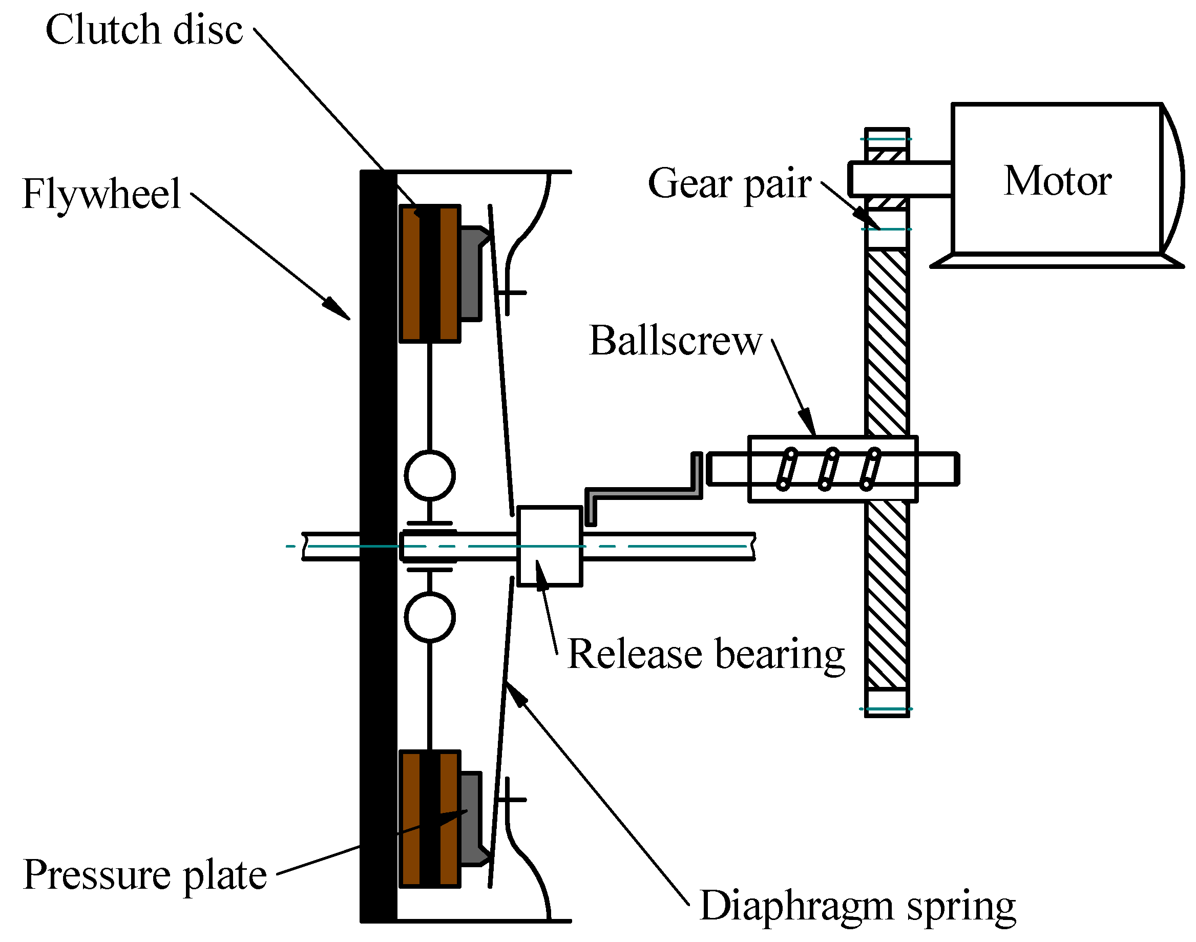
A schematic layout of a clutch mechanism and an electromechanical clutch actuator is shown in
Figure 1. In the engaged state, the diaphragm spring pushes the clutch disc to the flywheel through the pressure plate, and then the torque is transmitted via dry friction. By pushing the release bearing (or pulling in the case of pulled-type clutches), the axial force applied on the pressure plate by the spring starts to decrease. The clutch starts to slip if the axial force is small enough, but the elements are still connected. This is a partially engaged state, which is needed to start the vehicle or help with synchronization, although it also increases the wear rate of the clutch. The last state of the clutch is the disengaged state, when the elements are separated, hence there is no torque transmission.
The actuator consists of an electric motor connected to a mechanical linear actuator (typically a ballscrew thanks to its efficiency, although leadscrews are also mentioned in the literature) through a reduction gear pair. The threaded shaft of the ballscrew pushes the release bearing through a linkage. The clutch fork is connected to the release bearing, hence it can engage or disengage the clutch. A gap is kept between the release bearing and the actuator to detach the natural oscillations coming from the vehicle’s internal combustion engine from the system in the engaged state.
2.1. System Equations
In these applications, the control system can be divided into two controllers forming a cascaded control loop. The external loop is responsible for calculating the motor torque, which is needed to follow the requested position. Then, this torque serves as the reference for the internal loop. The inclusion of the clutch force is part of the external control loop, hence the motor model is simplified. It is assumed that the motor can follow the reference torque within its power limit:
where
is the maximum power of the motor and
is its angular velocity.
Similarly to modeling sensors, the motor’s dead-time, and control loop are also taken into account via a low-pass filter:
where
is equal to the time after which the output reaches 0.632 of the input step value.
The angular position of the motor is calculated according to Newton’s 2nd equation:
where
is the load torque generated by the clutch spring,
summarizes the frictional losses,
is the whole system’s inertia reduced to the motor shaft, and
is the position of the bearing.
The used friction model consists of the Coulomb-friction and viscous friction, where a sigmoid function describes the discrete, switching behavior of the Coulomb-friction:
where
is the Coulomb friction,
f is a scaling factor describing the gradient of the sigmoid function and
is the viscous friction coefficient.
The load force of the clutch is transmitted through the ballscrew and the gear pair, hence it is calculated as:
where
is the force of the diaphragm spring,
is the ballscrew’s lead,
is its efficiency and
is the torque ratio of the gears.
As the force of the diagram spring depends on the clutch position, the load torque will also be a function of it:
2.2. Clutch Characteristic Estimation
The clutch characteristic consists of a nominal force and a hysteresis generated by friction. Using only the nominal value of the clutch force simplifies the design procedure at the expense of accuracy. On the other hand, the controllers should be robust enough to compensate for the hysteresis effect.
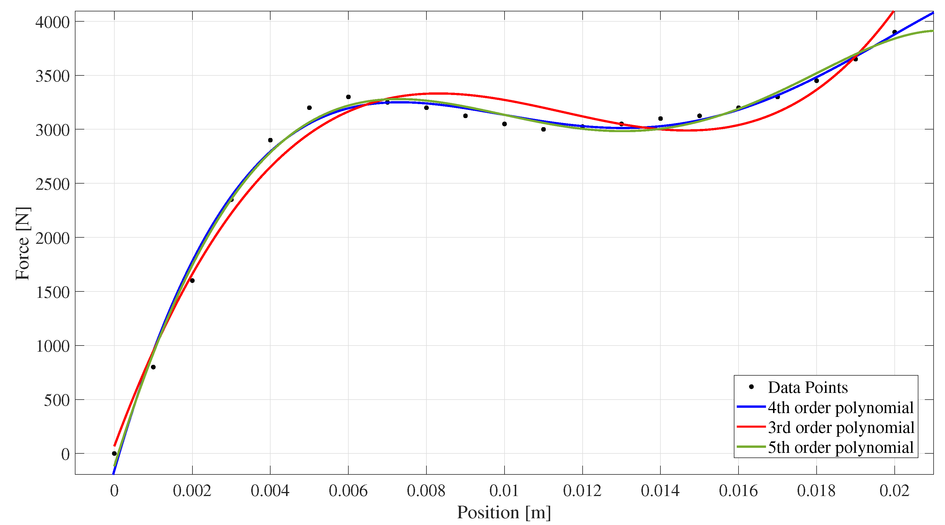
Based on [
4], a third-order polynomial could be used, but as is expected, increasing the order of the polynomial increases the accuracy of the curve fitting, hence a fourth-order and fifth-order polynomial has also been tested. The clutch force was measured with 1 mm resolution, then the linear least-squares method was used to determine the coefficients of the polynomials. The results of the curve fittings are shown in
Figure 2.
The root mean square error (RMSE) of different order polynomials are summarized in
Table 1. Because the fifth-order polynomial does not have a significant advantage concerning accuracy, the fourth order-polynomial has been chosen.
Further increasing the order of the polynomials could lead to more accurate results, but the reached accuracy is already within the hysteresis of a typical heavy-duty clutch; therefore, the fourth-order polynomial is acceptable for the analyzed clutch. The polynomials order can change as it must be determined according to the actual clutch characteristic and the desired accuracy, but the methodology remains the same regardless of the polynomial’s order.
Therefore, the clutch force is written as:
where
are the coefficients of the polynomial.
3. Methodology
3.1. Model Predictive Control
The MPC aims to find a future trajectory of the input signal, which optimizes the future behavior of the plant. The model used in the design process, in this case, is the discrete-time state-space representation of the system. To provide zero remaining error, the augmented state-space model is used, in which case the state vector is modified to contain the state increment and the system’s output, hence the controller can eliminate steady-state error.
Based on the state-space model, the predicted state variables are calculated sequentially using the set of future control parameters, from which the predicted outputs are calculated. In a compact matrix form, the series of predicted outputs are written as:
where
x(
k) is the state vector,
is the difference of the control variables,
F and
are matrices describing the prediction.
Therefore
that minimizes the following cost function must be calculated:
where
is the data vector containing the setpoint information, and
is the reference signal.
The necessary condition of the minimum cost is obtained as:
where
is a diagonal matrix containing the tuning parameter of the cost function,
F and
are matrices combining the state and output equations for the whole prediction horizon into a compact matrix form:
where
A,
B, and
C are the matrices of the augmented state-space model,
and
are the prediction and control horizons.
From which, the optimal control signal (
) is obtained as:
where
is the MPC gain and
is the system output gain, which is equal to the last element of
.
Although, this solution still does not include any restrictions regarding the control variables, their gradient, or the output of the system. The cost function in the presence of hard constraints is modified:
subject to the inequality constraints summarized as:
where
M and
are a matrix pair describing the inequality constraints.
Applying these constraints significantly increases the system’s performance. However, minimizing the cost function, including the constraints, leads to Hildreth’s Quadratic Programming algorithm, which is difficult to solve in embedded applications. Consequently, in these applications, the unconstrained cost function is used, in which case the feedback gain remains constant for Linear Time Invariant (LTI) systems, or it is described by a set of constant gains for gain-scheduled MPC algorithms.
3.2. Linear Parameter Varying Control
Linear Parameter-Varying systems are a class of nonlinear systems that are modeled as parametrized linear systems whose parameters change over time or with their states. In the literature, LPV systems are mostly described by using Linear Fractional Representation (LFR), polytopic models, and grid-based LPV models. LFR models use Linear Fractional Transformation (LFT) to separate the nonlinearities of the system from the nominal, LTI part of the system. Such nonlinearities can be time-varying parameters and uncertainties, but they can be used only in the case of rational parameter dependence. Polytopic models are often used to describe affine LPV systems, where the vector of parameters evolves inside a polytope, hence it is written as a convex combination of the polytope’s vertices. Grid-based LPV models divide the parameter domain into a grid of parameter values, then Jacobi linearization is applied to specify the linear dynamics at each grid point. They can handle any parameter representation, as they implicitly capture the system’s parameter dependence.
LPV systems are divided into two types based on the scheduling parameter vector. If the parameters are external (exogenous) variables, then the system is non-stationary, while if they are functions of the state variables (endogenous variables), then the system has nonlinear dynamics. LPV systems with endogenous parameters are also called quasi-LPV (qLPV) systems.
This paper chooses the grid-based representation, as it is also needed to calculate the state-dependent gains for the gain-scheduled MPC algorithm.
The state-space representation of a grid-based LPV model is written as:
where
is the state vector,
is the output vector,
is the input vector,
is the vector of scheduling parameters, and
A,
B,
C, and
D are parameter dependent matrices of the state-space representation.
3.3. State-Space Representation
While the nonlinear equations describing the system’s behavior have been reduced to the motor shaft, the state-space model has been written reduced to the release bearing. Under normal circumstances, these equations are proportional and differ only in a constant gain. As the aim is to include the diaphragm spring’s force in the state-space representation, it is more pragmatic to write the equations for linear movement. As the paper focuses only on position control, the state-space vector has been chosen as follows:
where
is the force generated by the motor at the release bearing.
The control signal is the force requested by the controller:
The output of the system is the position of the release bearing:
The general form of the given nonlinear system is formulated as:
where
x is the state vector,
y is the output vector,
u is the input vector,
d is the disturbance vector.
From the nonlinear equations, the state matrices are obtained via linearization, as follows:
where
A is the state matrix,
B is the input matrix,
C is the output matrix, and
D is the feedthrough matrix.
During Jacobi linearization, is an equilibrium point of the system. Although, from the definition of the grid-based LPV model comes to the fact, that the model should be linearized in several states. In this case, an equidistant division of the position has been used.
The state-space representation takes the dead-time of the motor and the torque control into account through
. Hence, after simplifying the friction force, the matrices of the state-space representation are written as follows:
As the state matrix is a function of the position, but it does not depend on any exogenous parameters, the presented representation is a quasi-LPV model, where the scheduling parameter vector has only a single element:
4. Controller Synthesis
4.1. Model Predictive Controller
Two MPC controllers have been designed to achieve the position control of the system. The first algorithm uses the linear state-space model of the actuator; therefore, the derivative of the load force has been omitted from the state matrix. The second algorithm uses the qLPV description of the system; therefore, the applied controller gain
is a function of the clutch position:
While this paper focuses on the LPV representation, given the characteristics of the system, using nonlinear MPC (NMPC) could also be a sensible choice. Solving the nonlinear optimization problem efficiently is a complicated task, although promising results have been presented recently. Such as [
25], where the
norm is used as it gives better control quality, but it can lead to a non-differentiable cost function. Hence, a neural approximator is used in place of the non-differentiable absolute value function, and an advanced trajectory linearization is performed online.
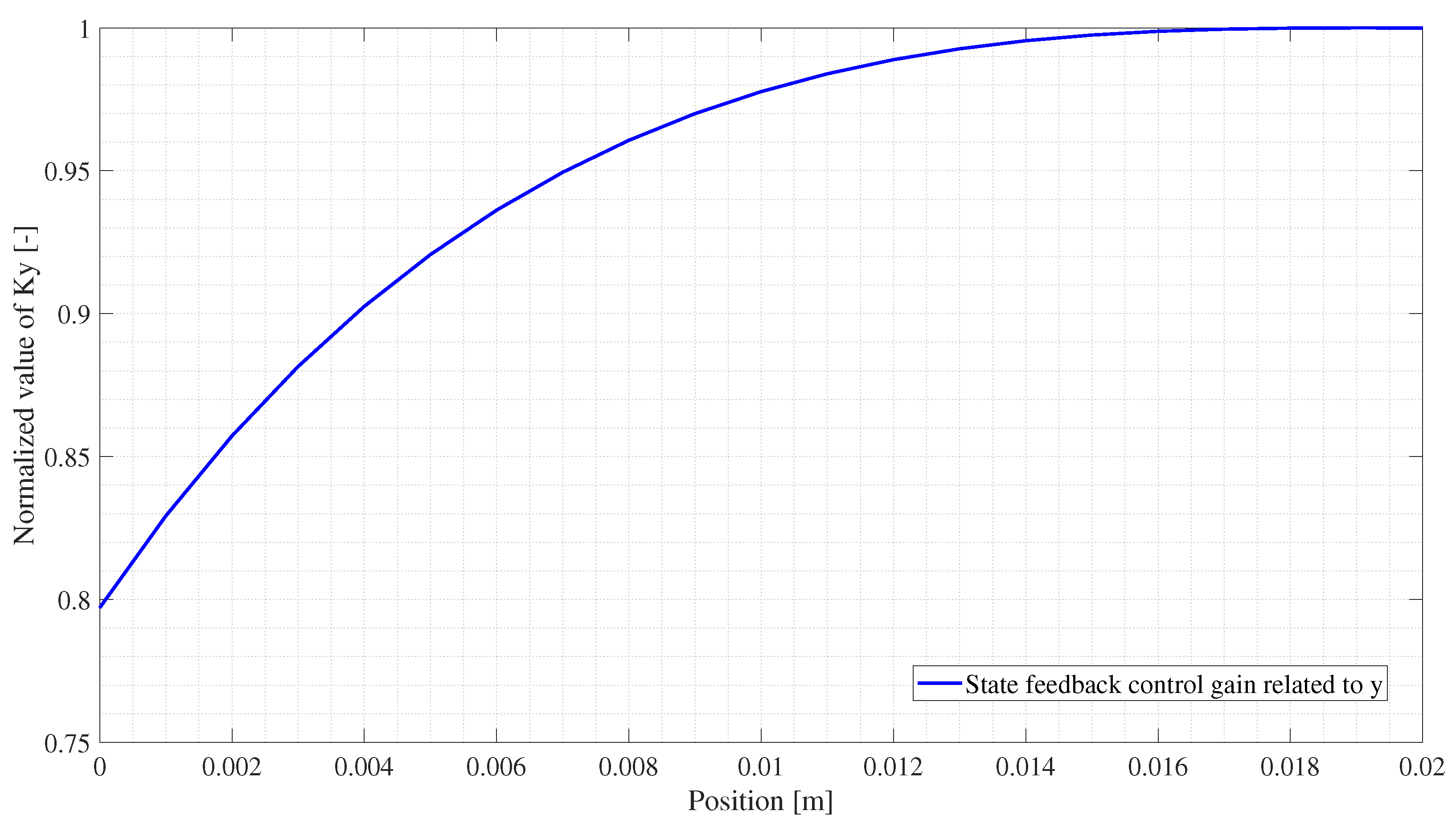
First, the standard MPC has been tuned using a step request. The tuning of the controller has been completed by changing . A higher weight means more expensive control, thus higher weights cause slower reference tracking. The tuning aims to find a trade-off between the control cost, tracking accuracy and overshoots, which meets the given time-domain requirements. To provide an accurate comparison, the determined weights have been fixed and used also in case of the gain-scheduled MPC.
Figure 3 shows the position dependency of the state feedback controller gain, based on which, the controller uses a slightly reduced parameter set when there is no load torque. This difference decreases in the case of cheaper controllers, while the shape of the function also changes slightly.
Besides comparing the linear MPC and the gain-scheduling MPC with different weights, these controllers could also be tested without constraints, while applying constraints on the output, input, and gradient of input significantly increase the performance and stability of the system, solving the optimization problem is not feasible in embedded applications. Hence, the next step of the research could be the analysis of the real-time applicability of the algorithms after which the needed limitations could be defined.
4.2. Linear Parameter Varying-H∞ Controller
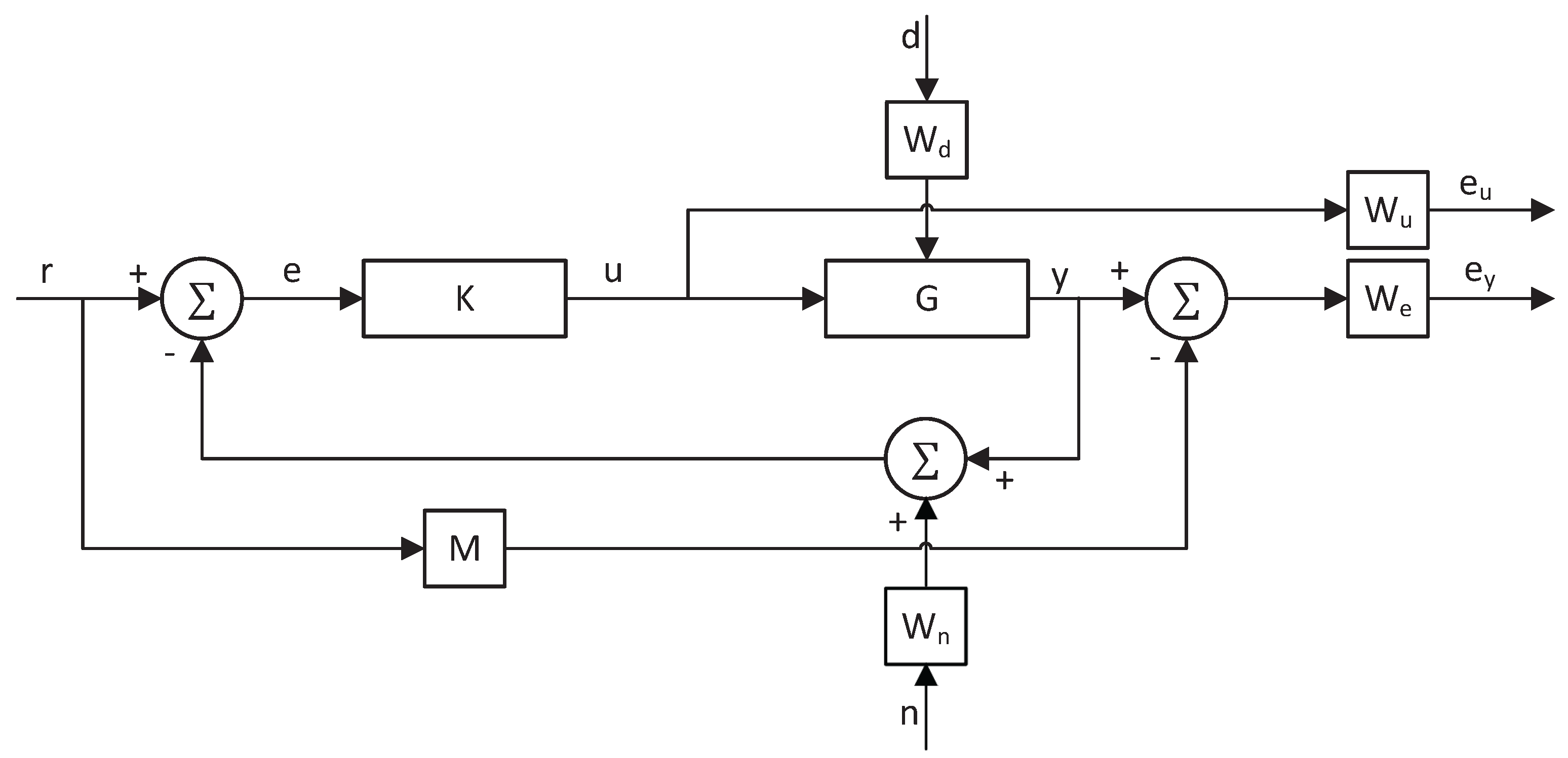
As the state-space representation of the actuator is already known, the next step is the formulation of the generalized plant. Its layout is shown in
Figure 4.
The system has a reference signal (r), a measurement noise (n), an input disturbance (d), and two output costs ( and ). Besides the controller (K) and the plant (G), the several weighting functions are also part of the generalized plant, which represent the model’s uncertainty and performance objectives.
The initial values of the performance weights have been selected using guidelines found in the literature, although they had to be refined using heuristic methods to achieve the desired performance.
is the control input weight. It is chosen as a high-pass filter to penalize the high-frequency content of the control signal, hence limiting the control bandwidth.A good approach is to choose
as the reciprocal of the maximum allowed input, but it must be optimized based on the results and the expected behavior of the system.
is the performance weighting function, which reflects the performance specifications of the closed-loop system. To find a trade-off between fast response time and low overshoot, the weight must have a low gain at low frequencies and a high gain at higher frequencies. The weighting function’s cross-over frequency shall be equal to the inverse of the desired closed-loop time constant. The initial estimation of
is the expected steady-state error of the system, which is the finetuned to meet the expected performance. The final weight has been written as:
models the sensor noise. As sensors are more accurate at low frequencies, it is modeled as a high-pass filter:
where the sensor’s accuracy is assumed to be 0.01 mm.
Constant 500 N disturbance is assumed to be on the system’s input, hence
describing the input disturbance is written as:
is utilized to include the time-domain requirements in the controller design. To have the expected disengagement time in case of a step request, the weight is formulated as:
After the generalized plant is formulated, the controller can be developed. To provide a robust solution, an LPV/H
∞ controller is synthesized using LPVtools [
26]. The H
∞ control design aims to minimize the induced
norm of the closed-loop system.
The controller synthesis in LPVtools has five main steps:
Defining the scheduling parameters as pgrid objects;
Defining the state matrices of the grid-based LPV model using the scheduling parameters;
Combining the state matrices to form the grid-based LPV model in pss data structure;
Creating the generalized plant by defining the weighting functions and connecting them using the sysic interconnection structure of Matlab Robust Control toolbox;
Controller synthesis using LPVsyn function of LPVtools.
While there are general methods, which give a good initial value of the controller parameters, the tuning of the controllers is an iterative process. The controllers have been tuned using heuristic algorithms on a step request, where the main goal was to find a trade-off between the rise time and overshoot.
5. Results
The applied test sequence consists of several parts: a disengagement of the clutch, holding the clutch in the disengaged position, engaging the clutch until reaching the touch-point, slipping the clutch to control the transmitted torque in partially engaged state, and then finishing the engagement.
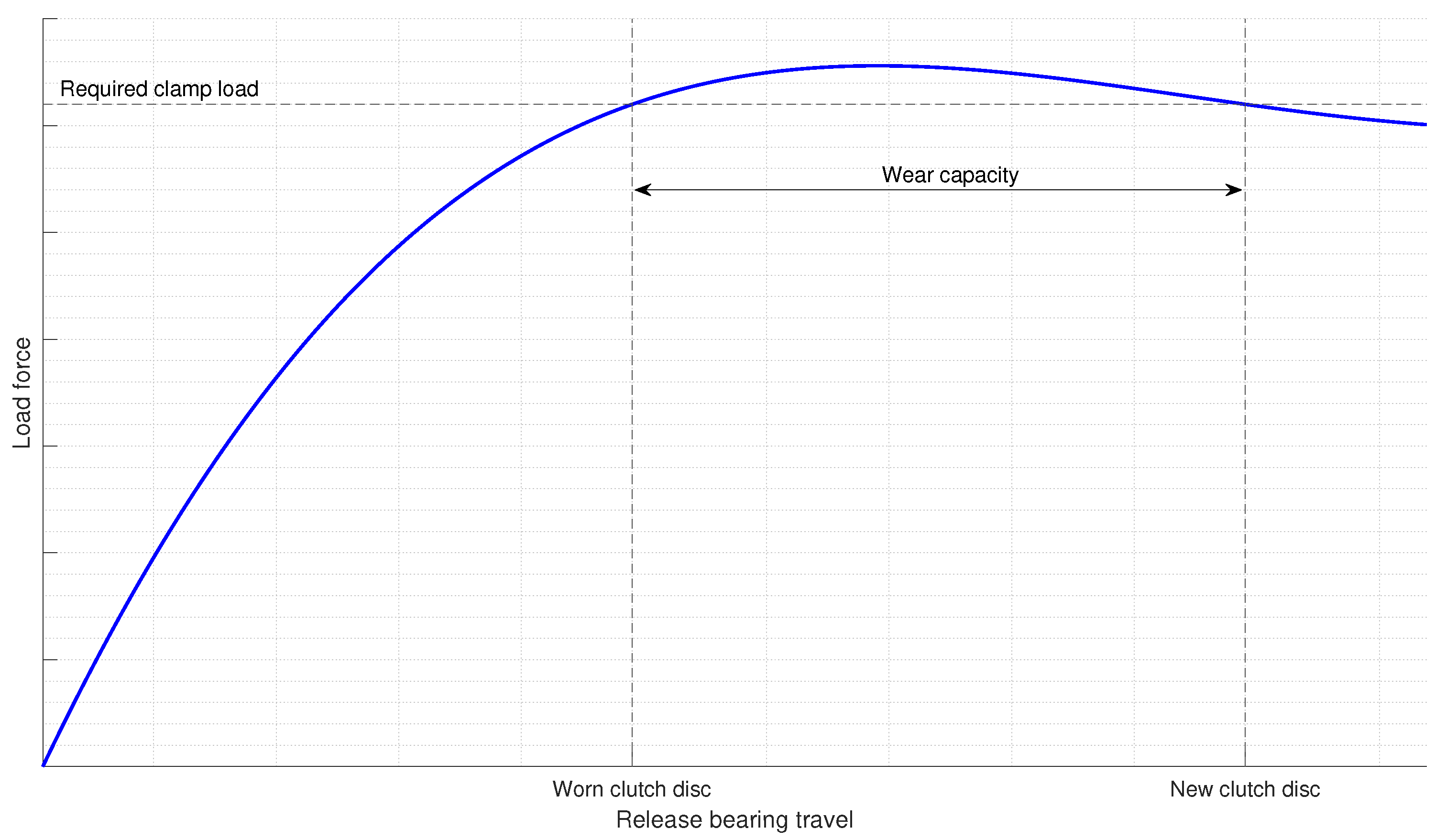
Due to the wear of the clutch disc, the load characteristic will also change, which is shown in
Figure 5. In the case of a new pressure plate assembly, the operating point (or touch-point) clutch is in the decreasing part of the diaphragm spring characteristic, where the required clamp load is the axial force needed to transmit the motor torque through the clutch.
As the clutch disc wears, the force corresponding to the operating point will start to increase, then it will eventually return to its original value after the wear limit has been reached. Further explanation about the phenomena is presented in [
27]. Hence, the controller must be robust to the changes of the touch-point and to the changes of the load force. Therefore, the sequence has been repeated two additional times assuming different touch-points.
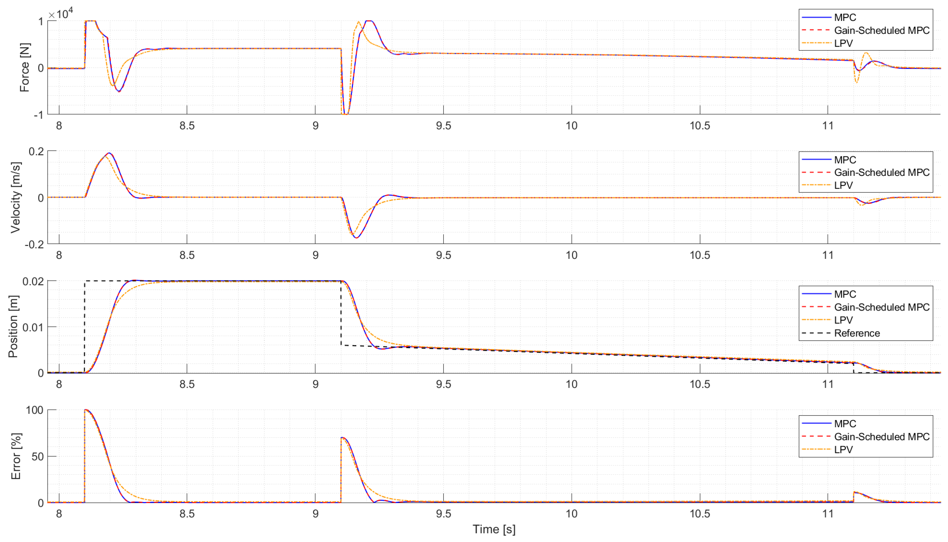
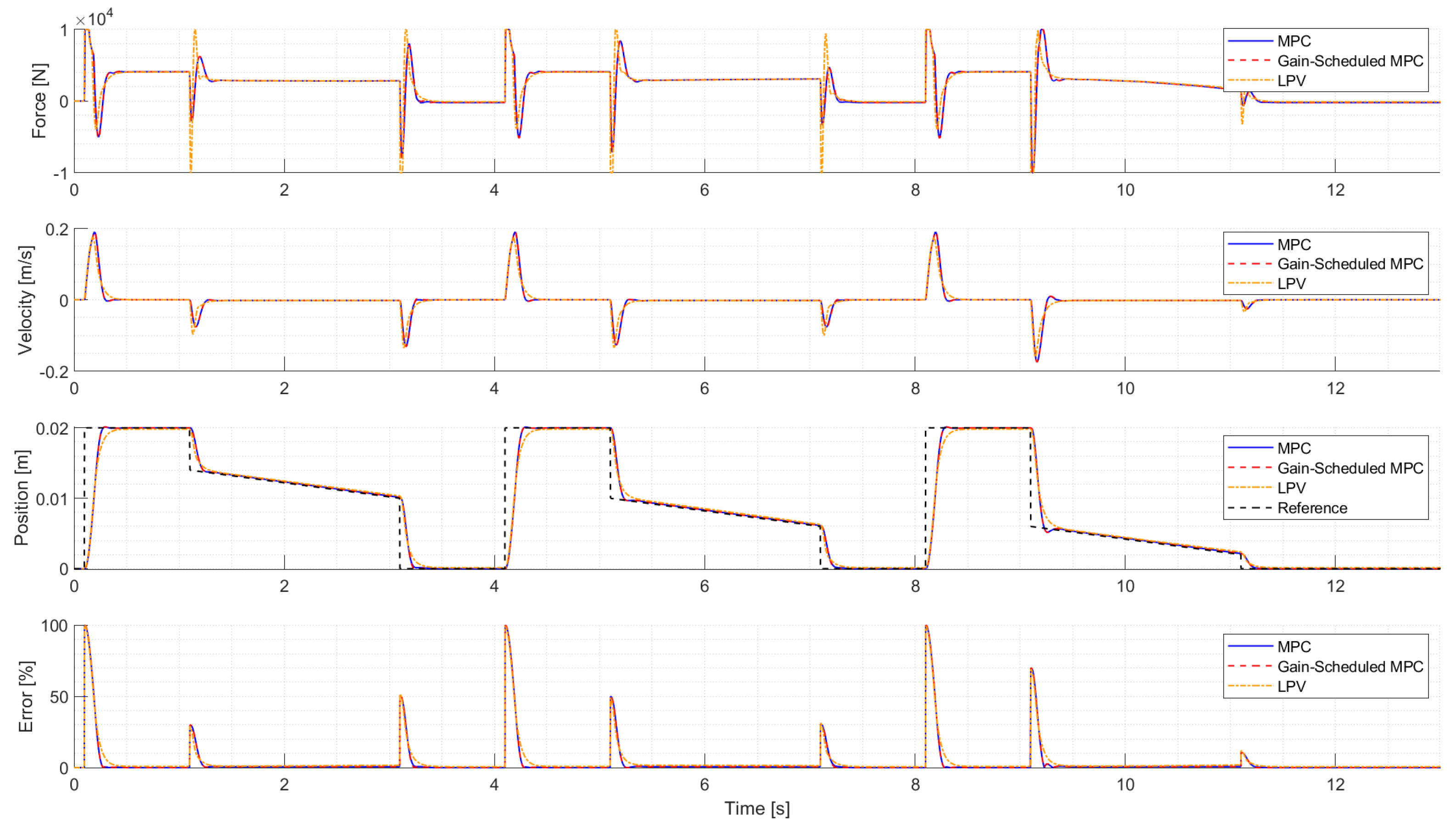
Figure 6 shows the comparison of the MPC, gain-scheduled MPC, and LPV-H
∞ controllers. The first diagram shows the force generated by the motor, the second diagram shows the velocity, the third and fourth diagrams present the actual and requested positions and the relative position error. Regarding the rise time, the MPC algorithms perform better by ca. 40 ms, but they also have minor overshoots and undershoots. The latter increases as the touch-point shifts towards the fully closed position. The LPV-H
∞ controller reacts faster when there is a new request, but its output also decreases earlier to prevent overshoot. On the other hand, the MPC is slower to react to the change in the request but starts to brake a bit later. Hence, it can achieve faster reference tracking with minimal over and undershoots.
The over and undershoots become crucial in the lowest slipping region, which is shown in
Figure 7. In the highlighted case, the undershoot exceeds 0.5 mm, which is already seen in the torque transmitted through the clutch. This scenario must be avoided as the transmitted torque severely affects both the vehicle dynamics and passenger comfort.
At first sight, there is no difference between the gain-scheduled and the linear MPC. The minor differences can only be seen around 0mm, where there is no significant load force, and the gain-scheduled algorithm uses reduced weights. Hence, it can provide smoother movement around this position. Although this difference is negligible because the clutch is already fully engaged, minor changes in the position do not affect the transmitted torque. The results of the comparison are summarized in
Table 2. As there is no difference between the MPC controllers in these aspects, they have been merged.
Applying a more expensive control would increase both over and undershoots, while cheaper strategies perform slightly better regarding the overshoot, but undershoots would be drastically worse.
Real Target Application and Future Challenges
While both algorithms have promising results in a simulation environment, their real-time application in an embedded environment is still a difficult challenge. In the case of the MPC algorithm, the unconstrained gains can be calculated offline, but solving the optimization problem online is not feasible in most cases. Significantly limiting the iteration number could lead to even worse results than using a simple unconstrained MPC with saturation, while enabling too high CPU load hence risking task re-entrants is not allowable in safety-critical applications, such as the presented clutch actuators.
Another solution could be the application of explicit MPC algorithms, where the computation performed online would be a simple function evaluation. In this case, the MPC controller is expressed as a lookup table of linear gains. The drawback of this solution is the same as that of the LPV controller. The number of parameters is limited by the memory of the ECU. Storing hundreds or thousands of parameters for a single controller is not viable; therefor, their size must be reduced at the cost of their performance.
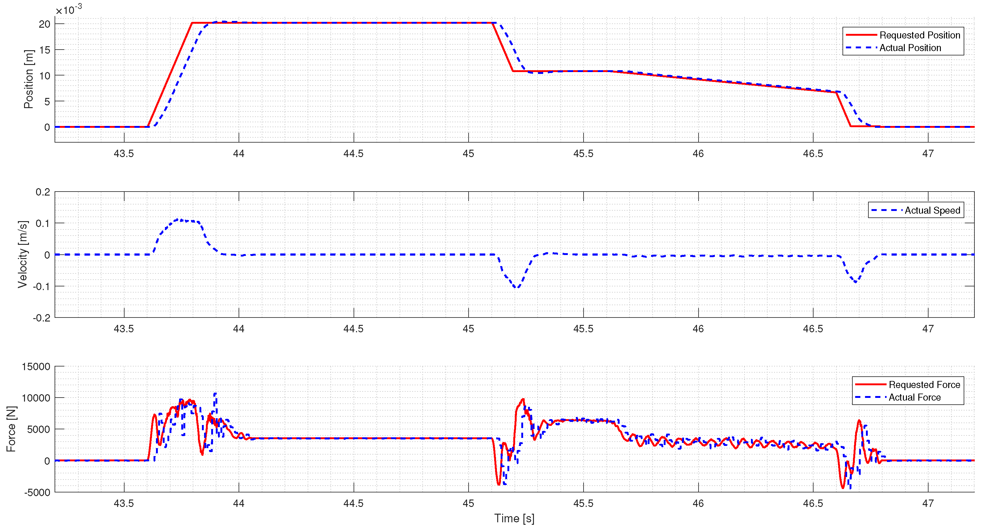
Based on the first results, with proper conditioning (e.g.,: applying max speed limits through the gradient of the reference signal) saturated MPC controllers can control the system with acceptable accuracy. Such an example is presented in
Figure 8. Due to the limitations of the electrical hardware, the disengagement time has increased significantly, but a minor overshoot and a more significant undershoot (0.5mm) can be seen in the measurements.
On the other hand, the controllers size must be significantly reduced. A possible solution is to reduce the controller’s order using model reduction techniques, such as the balanced order model truncation method. Another approach is to lower the resolution of the scheduling parameter vector, hence decreasing the number of LTI models consisting of the LPV model. In both cases, a trade-off must be found between the accuracy and the computational cost.
6. Conclusions
In this paper, a nonlinear model of an electromechanical clutch actuator has been presented, focusing only on the system’s mechanical dynamics. Then, a quasi-LPV representation of the system has been formulated, where the clutch position has been chosen as the scheduling parameter.
Using the qLPV representation of the actuator, a gain-scheduled MPC and an LPV-H∞ controller have been designed to achieve position control of the actuator. Furthermore, a linear MPC has also been developed using the same weights as the gain-scheduled MPC algorithm to serve as a benchmark. Assuming a nearly ideal electrical system and motor control algorithm, the developed controllers have been validated in a Model in the Loop environment using Matlab/Simulink.
Based on the results, the gain-scheduled MPC controller could only surpass the linear MPC in case of low positions, where there is no significant load force. This is caused by the decreased control parameter set used by the gain-scheduled MPC in this region. Although without load force there is no transmitted torque, hence this minor advantage is negligible.
The LPV-H∞ controller has a lower rise-time than the MPC controllers, but it is proven to be a more robust solution. It is less sensitive to the touch-point of the system, hence it is more suitable to control the actuator through its lifetime.
At last, some preliminary results and remarks are given regarding the real-time applicability of the presented methods.


