Majorization–Minimization Total Variation Solution Methods for Electrical Impedance Tomography

Abstract

Inverse problems arise in many areas of science and engineering, such as geophysics, biology, and medical imaging. One of the main imaging modalities that have seen a huge increase in recent years is the noninvasive, nonionizing, and radiation-free imaging technique of electrical impedance tomography (EIT). Other advantages of such a technique are the low cost and ubiquitousness. An imaging technique is used to recover the internal conductivity of a body using measurements from electrodes from the body’s surface. The standard procedure is to obtain measurements by placing electrodes in the body and measuring conductivity inside the object. A current with low frequency is applied on the electrodes below a threshold, rendering the technique harmless for the body, especially when applied to living organisms. As with many inverse problems, EIT suffers from ill-posedness, i.e., the reconstruction of internal conductivity is a severely ill-posed inverse problem and typically yields a poor-quality solution. Moreover, the desired solution has step changes in the electrical properties that are typically challenging to be reconstructed by traditional smoothing regularization methods. To counter this difficulty, one solves a regularized problem that is better conditioned than the original problem by imposing constraints on the regularization term. The main contribution of this work is to develop a general ${\ell }_p$ regularized method with total variation to solve the nonlinear EIT problem through a iteratively reweighted majorization–minimization strategy combined with the Gauss–Newton approach. The main idea is to majorize the linearized EIT problem at each iteration and minimize through a quadratic tangent majorant. Simulated numerical examples from complete electrode model illustrate the effectiveness of our approach.

1. Introduction

One of the most well-known techniques in the recent years to detect anomalies within the body is electrical impedance tomography (EIT). Such a technique has been of high interest in the medical imaging community since the publication of Calderón’s foundational paper that introduced the idea of applying external voltage patterns to an object; assuming that the medium is sufficiently close to a constant admittivity, the reconstruction can be directly accomplished by inverse Fourier transform [1,2]. EIT is a noninvasive, radiation-free, and low-cost experimental method for producing tomographic images from measurements obtained at the surface of an object. The procedure is as follows: a current is injected through electrodes that are placed on the boundary of the object of interest. Then, the resulting voltage is collected through the electrodes and produces the measured boundary data from which internal resistivity is reconstructed. There are many applications of EIT, including the detection of bodily tumors [3], the imaging of lung function [4], stroke monitoring [5,6], noninvasive medical imaging [7,8,9], nondestructive testing [10] and oil reservoirs [11,12]. Nevertheless, despite its popularity, the process of recovering reliable tomographic images is challenging and comes twofold: (1) the major issue to the EIT is that the inverse problem is highly nonlinear, and (2) it is very ill-posed from solving the higher dimensional problem using lower-dimensional data that are collected in the boundary (see for instance [13,14]). Voltage data (that we usually refer to as measurements) are usually highly corrupted with unknown levels of noise and type. Consequently, recovered solutions are highly sensitive to perturbations in the data, rendering the inverse problem challenging to solve. The ill-posedness of the solution is interpreted as small presence of the noise in the measurements usually causes high oscillations in the available data. The setup that we adopted here is as follows: We consider attaching L electrodes on the surface $\partial \Omega$ of a body $\Omega$ with conductivity $\mathbf{x}$. The current is injected into the body through electrodes, and resulting voltages are measured through the same conductor. Electrodes are placed on the surface of the body that is called boundary $\partial \Omega$ here, and we denote the subset of the boundary where the electrodes are placed by $e_{\ell }$, $1\le \ell \le L$. We denote the current applied to $e_{\ell }$ by $I_{\ell }$. A vector $I={(I_1,I_2,\dots ,I_L)}^T$ is called current pattern if it satisfies the law of conservation of charge, i.e.,

$$\sum _{\ell =1}^L{I}_{\ell }=0.$$

(1)

The corresponding voltage pattern is denoted by $V={(V_1,V_2,\dots ,V_L)}^T$, such that

$$\sum _{\ell =1}^L{V}_{\ell }=0.$$

(2)

We refer the reader to [15] and references therein for more details on the current patterns on the EIT problem. The EIT problem is well-studied and there exists a rich literature discussing challenges and a variety of solution methods starting from nonlinear methods such as Gauss–Newton [16] to D-bar methods [17], and more recently learning approaches through neural networks (NN) [18]. Nevertheless, to overcome the challenges that arise in a poorly posed EIT inverse problem, there is a significant amount of research in the literature dedicated to a wide range of methods from deterministic to statistical, learning to improve recovered tomographic images. One of the most used methods in EIT are deterministic approaches that include iterative and direct methods by minimizing a certain well-defined functional, such as least-squares fitting or more general formulation methods (Tikhonov regularization and D-bar type methods) [13,14]. Other well-known approaches include the factorization method [19] and D-bar type methods [20,21]. Such methods are applicable to a wide selection of problems in EIT, independently from specific types of conductivity distributions. There exists a wide literature that such methods can also be applied to cases with a mix of conductive and resistive targets to reconstruct [22].

Other methods that have recently become popular for the EIT problem include statistical inversion methods [23], which have started to play a significant role in quantifying the uncertainties of the EIT reconstruction. In [24] the authors attempted to quantify the effects of these measurement errors on EIT reconstruction. They developed a comprehensive framework that combined uncertainty quantification techniques and EIT reconstruction techniques. Further, in [25] is proposed an approach that was used to optimize the current patterns on the basis of criteria that are functions of the posterior covariance matrix. There is also some research studying errors due to model reduction and concerning partially unknown geometry using the Bayesian approach [26,27].

Paper Overview

The paper is organized as follows: Section 2 outlines the notation and background that are needed throughout this paper. Additionally, we discuss the complete electrode model as our choice for solving the EIT forward problem, present the finite element method to discretize the infinite dimensional problem, and formulate the inverse problem of interest. Furthermore, we state the need for regularization and particularly total variation regularization. Next, we give some background on TV-type methods and explain the motivation for the choice of the method that we present in this paper. In Section 3, we formulate the EIT inverse problem as a minimization problem. We proceed to introduce our first method, a TV- and MM-based approach that is combined with a Gauss–Newton method to iteratively reweigh nonlinear problems. Next, we also introduce a fractional total variation method. Lastly, in Section 4 we illustrate the performance of our method with numerical examples. In Section 5, we present some concluding remarks and future outlook for research. Main contributions: The main contributions of this paper are as follows:

1.

We propose an iteratively reweighted method through a majorization–minimization (MM) technique to solve the general ${\ell }_p$ regularization EIT problem for a broad selection of the values of p, i.e., $0<p\le 2$.

2.

We combine the MM method with the IRGN to solve the nonlinear EIT inverse problem.

3.

We include a general regularization operator $\Theta$ for specific choices and values of p (on which we comment here) yielding different methods. For instance, choosing $p=1$ yields TV-MMIRGN, and choosing $0<p<1$ yields the FTV-MMIRGN method.

4.

We test our methods on simulated examples that involve conductive and resistive anomalies.

2. Background and Formulation of Problem of Interest

In this section, we establish the background and notation, and formulate the problem to solve in this paper.

2.1. Electrode Model

The EIT can be modelled using different electrode models [28]; some of the most significant models in EIT are continuum, point electrode [29], shunt [30] and complete electrode models (CEM) [31]. The point electrode model considers an L electrode system of negligible size, and the system satisfies the consistency condition. The so called shunt model correctly models the geometry of the electrodes, but neglects the thin resistive layer that may appear at the contact between electrodes and object [32]. It can be modelled as the limit of the CEM when contact resistances tend to zero [33]. In this section, we discuss the complete electrode model, which is considered to be one of the most accurate models, since measured potentials can be predicted at the precision of the measurement system [34]. It simultaenously takes into account the effects of electrodes, and contact impedances between object and the electrodes [28,34,35]. We suppose that in the body are fixed L electrodes. Electric current is applied at pairs of electrodes, and the resulting voltage is measured at all the others. The process of injecting current and measuring voltage in other electrodes is repeated until sufficiently good characterization of the body is obtained. The inverse problem is to reconstruct the internal conductivity distribution from measurements places in its surface. Electromagnetic fields within the body can be modelled by Maxwell’s equation (see [36] for more details). The following formulation can be found in an extended list of references that we include here.

The complete electrode model is formulated as follows:

$$-\mathrm{d}\mathrm{i}\mathrm{v}(\mathbf{x}\nabla u)=0\mathrm{i}\mathrm{n}\Omega ,$$

$$\begin{array}{ccc}\hfill {\int }_{E_{\ell }}\mathbf{x}\frac{\partial u}{\partial n}dS& =& I_{\ell }^c\mathrm{o}\mathrm{n}{E}_{\ell },\ell =1,\dots ,L,\hfill \\ \hfill u+c_{\ell }\mathbf{x}\frac{\partial u}{\partial n}& =& U_{\ell },\mathrm{o}\mathrm{n}{E}_{\ell },\ell =1,\dots ,L,\hfill \end{array}$$

(3)

and the current density on the boundary between the electrodes satisfies

$$\mathbf{x}\frac{\partial u}{\partial n}=0,\mathrm{on}\partial \Omega \backslash {\cup }_{\ell =1}^L{E}_{\ell },\ell =1,\dots ,L,$$

where inside $\Omega$, there is no current source for the conductivity $\mathbf{x}\in L^{\infty }(\Omega )$ with $0<{\mathbf{x}}_1\le \mathbf{x}\le {\mathbf{x}}_2<\infty$. The area of the surface electrode ℓ is denoted by $E_{\ell }$. Moreover, the electrical current injected at the ℓ-th electrode is given by $I_{\ell }^c$. Lastly, quantity $U_{\ell }$ represents the measured electric potential, and $c_{\ell }$ is the effective contact impedance for the ℓ-th current pattern. Charge conservation law [37] ${\sum }_{\ell =1}^L{I}_{\ell }^c=0$ guarantees the existence of a solution to the problem that we are interested in solving (3). There are two important quantities of interest, such as the choice of a ground that is given by ${\sum }_{\ell =1}^L{U}_{\ell }=0$. Such a condition is used to guarantee that the obtained solution is unique. One of the main advantages of the complete electrode model given by (3) is that it simultaneously takes onto account the effects of the electrodes and the contact that is typically produced at the surface of the object. We direct the reader to the following references for more details [28,34,35]. A typical EIT setup requires some current $I^c$ to be injected into the interior of a medium from a set of electrodes. The resulting voltages, also known as measurements $V_{\partial \Omega }$, can be collected at the remaining electrodes. In practical settings, a wide range of experiments that use different input currents were developed. The main question of interest is on determining an approximation to $\mathbf{x}$ from limited knowledge of the Neumann-to-Dirichlet (NtD) map [36,38]. The next step is to apply the well-known variational form for the complete electrode model in (3) with which we formulate the variational equation; see, for instance, [35] for a complete discussion, as we omit the details here.

We obtain the following formulation:

$$\mathsf{\Gamma }((u,U),(v,V))=\sum _{k=1}^L{I}_k^c{V}_k,\forall (v,V)\in {\tilde{S}}^1(\Omega )=S^1(\Omega )\oplus {\mathbb{R}}_0^L.$$

(4)

Quantity ${\mathbb{R}}_0^L=\{(y_1,\dots ,y_L)\in {\mathbb{R}}^L:{\sum }_{i=1}^L{y}_i=0\}$, $\mathsf{\Gamma }:{\tilde{S}}^1(\Omega )\times {\tilde{S}}^1(\Omega )\to \mathbb{R}$ represents a bilinear operator, such that

$$\mathsf{\Gamma }((u,U),(v,V))={\int }_{\Omega }\mathbf{x}\nabla u·\nabla vdy+\sum _{\ell =1}^L\frac{1}{c_{\ell }}{\int }_{E_{\ell }}(u-U_{\ell })(v-V_{\ell })dS.$$

(5)

2.2. Discretization

For the convenience of the reader, we include the dicretization process here. One of the well-known methods that can be used to turn the infinite dimensional equation (continuous) of EIT problem into a finite dimensional (discrete) formulation is the finite elements method. Let $T=\{T_1,T_2,\dots ,T_N\}$ represent the triangles of region $\Omega$, and we consider N mesh points for the finite dimensional subspace $S_N$ of $S_1(\Omega )$. The potential distribution $u_N\in S_N$ is represented by

$$u_N\approx \sum _{i=1}^N{\gamma }_i{\psi }_i\left(x\right),$$

(6)

where ${\gamma }_i\in \mathbb{R}$, and ${\psi }_i\left(x\right)$ are basis functions of $S_h$ that are set to satisfy the equation ${\psi }_i\left(x_k\right)={\delta }_{i,k}$, for $i,k=1,2,\dots ,N$. The current potential on the electrodes is given by

$$U^N=\sum _{k=1}^{L-1}{\beta }_k{\varphi }_k=C\beta ,$$

(7)

where ${\varphi }_k,k=1,2,\dots ,L-1$ defines a basis for ${\mathbb{R}}^l$ and $C\in {\mathbb{R}}^{L\times (L-1)}$. Given the fixed current vector I and the positive contact impedance ${\left(c_k\right)}_{k=1}^L$, we define

$$\mathcal{G}:\mathcal{Q}\in L^{\infty }\to S,$$

(8)

where $\mathbf{x}\mapsto (u,U)$ is conductivity, and $\mathcal{G}$ is the forward operator that maps conductivity to the solution of the EIT problem. We briefly include the discretization process here for the convenience of the reader; more details on the discretization process and the errors that arise from the discretization can be found here [39].

2.3. Problem Formulation (Inverse Problem of Interest)

In this section, we formulate the problem to solve as a nonlinear least-squares problem and motivate the need for regularization. The forward problem with forward operator represented by $\mathcal{G}$ as in (8) uses unknown conductivity distribution $\mathbf{x}$ and finds boundary data that are associated with electrodes placed on the surface of the object of interest. The goal of the inverse problem in which we are interested here is to reconstruct conductivity distribution $\mathbf{x}$ and the resulting voltage vectors $U\in {\mathbb{R}}^L$ from the measured voltage data. We can formulate the forward model with the following equations:

$$\mathcal{G}\left(\mathbf{x}\right)=u^{\delta }.$$

(9)

${\mathbf{u}}^{\delta }=\mathbf{u}+ϵ$, where ${\mathbf{u}}^{\delta }$ represents available measurements that typically have the presence of some noise $ϵ$. Vector $\mathbf{u}$ represents the unknown vector (assumed to be error-free) that is associated with available data ${\mathbf{u}}^{\delta }$. Operator $\mathcal{G}$ is nonlinear and generally severely ill-posed; therefore, we seek to minimize the functional

$$\underset{\mathbf{x}\in {\mathbb{R}}^n}{min}{\parallel \mathcal{G}\left(\mathbf{x}\right)-{\mathbf{u}}^{\delta }\parallel }_2^2.$$

(10)

Severely ill-posed problems have solutions with particular properties. If solutions exist, they are very sensitive to the perturbations in the available data. The well-known technique to remedy such difficulties is to replace the original problem with a nearby regularized problem, whose solution is less sensitive to error in the data. The regularized problem in which we are interested can be written in the form

$$\underset{\mathbf{x}\in {\mathbb{R}}^n}{min}\mathcal{J}\left(\mathbf{x}\right)=\underset{\mathbf{x}\in {\mathbb{R}}^n}{min}\parallel \mathcal{G}\left(\mathbf{x}\right)-{\mathbf{u}}^{\delta }{\parallel }_2^2+\lambda {\parallel \Theta (\mathbf{x}-{\mathbf{x}}^{*})\parallel }_p^p,$$

(11)

where $\lambda$ is the regularization parameter that defines the trade-off between the first term in (11) (data-fidelity term that is also known as a fit-to-data term) and the regularization term. ${\mathbf{x}}^{*}$ represents known background conductivity, and $\Theta \in {\mathbb{R}}^{s\times n}$ is a nonsingular matrix that is known as the regularization operator. Functional $\mathcal{J}\left(\mathbf{x}\right)$ for $p=2$ and $\Theta \ne \mathbf{I}$ represents the generalized Tikhonov regularization [40] method that is one of the most popular regularization techniques. In this work, we develop a fractional generalized Tikhonov regularization method and total variation type method (with $\Theta \ne \mathbf{I}$) for EIT, which we describe below. When the bound of the noise is known, then one can use the discrepancy principle to define a regularization parameter $\lambda$. For convenience (since our focus is not on exploring different methods to define the regularization parameter in (20)), we assumed that the bound for the error of the noise was known:

$$\parallel {\mathbf{u}}^{\delta }{-\mathbf{u}\parallel }_2<\delta .$$

(12)

When the bound of the noise is not known, other techniques to find the regularization parameter, such as generalized cross-validation (GCV) or the L-curve, can be used (see [41,42]).

The main approach in this paper is considering the linearization of a nonlinear problem and developing methods on the basis of that approach. We skip details on the linearization process and the computation of the Jacobian matrix, but the interested reader can find details in [43].

The linearized version of forward problem (9) is given by

$$\mathbf{J}\left({\mathbf{x}}_k\right)\mathbf{x}=u^{\delta },$$

(13)

where $\mathbf{J}\left({\mathbf{x}}_k\right)$ represents that Jacobian matrix as an approximation at iteration k. In the linearized problem, our goal is to minimize the linear and discrete functional

$${\mathcal{T}}_k\left(\mathbf{x}\right)={\parallel \mathbf{J}\left({\mathbf{x}}_k\right)\mathbf{x}-u^{\delta }\parallel }_2^2.$$

(14)

Need for Regularization

We emphasize the need for regularization for the EIT problem. Because of the stability issues that arise in the ill-posed problems, small errors in the available data cause large oscillations in the reconstructed inverse solution. To remedy stability issues, one of the most popular techniques, Tikhonov regularization, substitutes the main ill-posed problem with a nearby solution that is less sensitive to the errors in the data. Such a process is called regularization. We refer the reader to [44] for an introduction to discrete ill-posed problems.

2.4. Total Variation Methods

In this subsection, we discuss the idea of total variation (TV) for EIT problems. It has been extensively used in a variety of problems including EIT in recent years. The use of TV helps to preserve discontinuities in the reconstruction such as sharp changes in conductivity distribution and boundaries of the perturbations that are in practice smoothed by the use of Tikhonov-type regularization terms. Nevertheless, the use of TV causes other difficulties, such as the nondifferentiability of the TV regularization term. A wide range of methods are used to address nondifferentiability, such as alternating direction method of multipliers (ADMM) and the primal dual interior point method (PDIPM). In this work we are interested in a more general TV regularization that also handles an ${\ell }_p$ regularization term. In the following paragraphs, we describe in more detail TV and the general regularization term that we propose in this work.

Total Variation on a Regular Rectangular Domain

Total variation (TV) regularization is a sparse representation of the gradient of the solution that was proposed for image denoising [45] and is applied in a wide group of imaging problems (see [46] for a review). Total variation has two main representations: isotropic and anisotropic total variation, where the first is invariant to the domain rotation, and the latter is not; hence, being rotationally nonsymmetric affects the edges to align with the coordinate axes. Given a vector $\mathbf{x}\in {\mathbb{R}}^n$ that represents a discrete two-dimensional image with the number of pixels $n=n_x\times n_y$, we define the discretization of the derivative operator

$${\mathbf{L}}_d=\left[\begin{array}{ccccc}1& -1& & & \\ & 1& -1& & \\ & & \ddots & \ddots & \\ & & & 1& -1\end{array}\right]\in {\mathbb{R}}^{(n_n-1)\times n_n},$$

(15)

where $d=x,y$, and we define ${\mathbf{I}}_{n_n}\in {\mathbb{R}}^{n_n\times n_n}$ with $n_n=n_x,n_y$. Consider the derivative matrix as

$${\mathbf{L}}_s=\left[\begin{array}{c}{\mathbf{I}}_{n_x}\otimes {\mathbf{L}}_y\\ {\mathbf{L}}_x\otimes {\mathbf{I}}_{n_y}\end{array}\right].$$

(16)

We use one of the most well-known formulations of discrete total variation, anisotropic total variation. We define $\mathbf{x}=mat\left(\mathbf{X}\right)$, where $mat(·)$ denotes the operator that converts the vector $\mathbf{x}\in {\mathbb{R}}^n$ into a matrix $\mathbf{X}\in {\mathbb{R}}^{n_x\times n_y}$. Anisotropic TV is then given by

$$\begin{array}{cc}\hfill TV\left(\mathbf{x}\right)& =\sum _{i=1}^{(n_y-1)}\sum _{\ell =1}^{n_x}\left|{\left({\mathbf{L}}_y\mathbf{X}\right)}_{i,\ell }\right|+\sum _{i=1}^{(n_x-1)}\sum _{\ell =1}^{n_y}\left|{\left(\mathbf{X}{\mathbf{L}}_x^T\right)}_{i,\ell }\right|\hfill \\ \hfill & =\parallel ({\mathbf{I}}_{n_x}\otimes {\mathbf{L}}_y){\mathbf{x}\parallel }_1+\parallel ({\mathbf{L}}_x\otimes {\mathbf{I}}_{n_y}){\mathbf{x}\parallel }_1={\parallel {\mathbf{L}}_s\mathbf{x}\parallel }_1.\hfill \end{array}$$

(17)

2.5. Total Variation and the Graph Perspective

In this paragraph, we describe the total variation on a finite element mesh following a graph perspective, in particular given a finite element mesh that is formed by $m_{\ell }$ elements. We consider an undirected and unweighted graph $G=V, E, M$ where the three components stand for a set of vertices V such that the number of the vertices is $m_{\ell }$ (i.e., $\left|V\right|=m_{\ell }$), the set of edges E, and a matrix M that is a weighted adjacency matrix. A vertex $v_i$, $i=1,2,\dots ,m_{\ell }$ in the graph represents the ith triangular element and is located at the center of the gravity of the current element. An edge $e_{i,j}\in E$ in the graph represents a connection between two vertices $v_i$ and $v_j$ on the triangle element. It is common that we assign a weight $a_{i,j}$ that is the length of the edge $e_{i,j}$. We can save information of the weighted connectivity in the weighted adjacency matrix $M\in {\mathbb{R}}^{\left|E\right|\times \left|E\right|}$ such that

$$M_{i,j}=\left\{\begin{array}{c}{a}_{i,j}\mathrm{i}\mathrm{f}{v}_i\mathrm{connected}\mathrm{with}{v}_j\hfill \\ 0\mathrm{else}.\hfill \end{array}\right.$$

(18)

2.5.1. Total Variation on a Graph

In this section, we describe the total variation on a triangular mesh. The TV operator is the discretization of the differential operator on undirected graphs we introduce the following matrix called the indication matrix $D\in {\mathbb{R}}^{\left|E\right|\times \left|V\right|}$

$$D_{e_{i,j},v_k}=\left\{\begin{array}{c}1/|e_{i,j}|\mathrm{if}i=k\hfill \\ -1/|e_{i,j}|\mathrm{if}j=k\hfill \\ 0\mathrm{else}\hfill \end{array}\right.$$

(19)

where $|e_{i,j}|$ is the length of edge $e_{i,j}$. Information about an undirected weighted graph can be characterized in adjacency matrix M. Regularization total variation operator $\Theta$ for this case is $\Theta =M·D$. More specifically, solving minimization problem (20) with TV regularization can be formulated as follows:

$$\underset{\mathbf{x}\in {\mathbb{R}}^n}{min}\mathcal{J}\left(\mathbf{x}\right)=\underset{\mathbf{x}\in {\mathbb{R}}^n}{min}\parallel \mathcal{G}\left(\mathbf{x}\right)-{\mathbf{u}}^{\delta }{\parallel }_2^2+\lambda {\parallel \Theta (\mathbf{x}-{\mathbf{x}}^{*})\parallel }_1,$$

(20)

where $\Theta =M·D$.

2.5.2. Fractional TV

Recently, using fractional TV regularization was shown to improve the quality of the obtained reconstructed solution by considering techniques from fractional calculus (see [47,48] and references therein). The order of regularization plays an important role in the trade-off between data fidelity and the regularization term. Oversmoothing (smoothing out the edges in the reconstruction) appears when a first-order term is employed. However, a high-order term usually causes noise. To achieve a good trade-off between terms, inspired by previous work in imaging [49], we introduce a fractional-order regularization [47] component into TV-based algorithm FTV_MMIRGN.

3. Fractional TV Solution Method for EIT FTV-MMIRGN

In this section, we discuss the main method that we propose in this work. Consider the nonlinear minimization problem in (20).

Given an initial approximation of desired solution ${\mathbf{x}}^0$ and guessed ${\mathbf{x}}^{*}$ for background conductivity, we consider the linearized functional

$$\underset{\mathbf{x}\in {\mathbb{R}}^n}{min}\mathcal{F}\left(\mathbf{x}\right)=\underset{\mathbf{x}\in {\mathbb{R}}^n}{min}\frac{1}{2}{\parallel \mathbf{J}\mathbf{x}-\widehat{{\mathbf{u}}^{\delta }}\parallel }_2^2,$$

(21)

where ${\widehat{\mathbf{u}}}^{\delta }={\mathbf{u}}^{\delta }-\mathcal{G}\left({\mathbf{x}}^0\right)+\mathbf{J}{\mathbf{x}}^0$ and ${\mathbf{J}}_0=\mathbf{J}\left({\mathbf{x}}^0\right)$. In the following paragraphs, we discuss the linearization process through the Gauss–Newton method. $\mathbf{r}\left(\mathbf{x}\right)=\mathcal{G}\left(\mathbf{x}\right)-{\mathbf{u}}^{\delta }$ is defined to be the residual, and requiring to solve (10) is equivalent to minimizing the residual error. In this paper we are interested in Gauss–Newton-type methods that include the computation of the Jacobian; hence, we compute the Jacobian matrix of the residual $\mathbf{r}\left(\mathbf{x}\right)$ as follows:

$${\mathbf{J}}^{\left(r\right)}{\left(\mathbf{x}\right)}_{i,j}=\frac{\partial \left({\left({\mathbf{u}}^{\delta }\right)}_i\right)-{\mathcal{G}}_i\left(\mathbf{x}\right)}{\partial {\mathbf{x}}_j}=-\frac{\partial \left({\mathcal{G}}_i\left(\mathbf{x}\right)\right)}{\partial {\mathbf{x}}_j}=-{\mathbf{J}}_{i,j},$$

(22)

where $\mathbf{J}$ represents the Jacobian of function $\mathcal{G}\left(\mathbf{x}\right)$ and the Hessian matrix of $\mathcal{G}\left(\mathbf{x}\right)$ for the same argument as above is

$${▿}^2{\mathcal{G}}_i\left(\mathbf{x}\right)={▿}^2{\mathbf{r}}_i\left(\mathbf{x}\right)={\mathbf{H}}_i,$$

(23)

where $\mathbf{H}$ is the notation we use to denote the Hessian of $\mathcal{G}\left(\mathbf{x}\right)$. Further, we use notation ${\mathbf{J}}_k$ to denote the Jacobian of $\mathcal{G}\left(\mathbf{x}\right)$ at $\mathbf{x}={\mathbf{x}}^{\left(k\right)}$. The computation of the Hessian matrix is computationally expensive; hence, a typical remedy is to approximate the Hessian of $\mathcal{F}\left(\mathbf{x}\right)$ in the form

$${▿}^2\mathcal{F}\left(\mathbf{x}\right)\approx \mathbf{J}{\left(\mathbf{x}\right)}^T\mathbf{J}\left(\mathbf{x}\right).$$

(24)

Such approximation is appropriate if the initial approximate solution ${\mathbf{x}}^{\left(0\right)}$ is close to the ${\mathbf{x}}^{*}$ that implies an approximate solution $\widehat{\mathbf{x}}$ that satisfies $\mathbf{r}\left(\mathbf{x}\right)={\mathbf{u}}^{\delta }-\mathcal{G}\left({\mathbf{x}}^{\left(0\right)}\right)$. A similar strategy is followed to linearize nonlinear forward operator $\mathcal{G}\left(\mathbf{x}\right)$ around a neighborhood of ${\mathbf{x}}^{\left(k\right)}$ at iteration k. As an initial step, we approximate $\mathcal{G}\left(\mathbf{x}\right)$ abound the initial approximation ${\mathbf{x}}^{\left(0\right)}$ as

$$\mathcal{G}\left(\mathbf{x}\right)\approx \mathcal{G}({\mathbf{x}}^{\left(0\right)})+\mathbf{J}({\mathbf{x}}^{\left(0\right)})(\mathbf{x}-{\mathbf{x}}^{\left(0\right)}),$$

(25)

where $\mathbf{J}$ is the Jacobian of $\mathcal{G}$. The Gauss–Newton iteration to solve (10) can be written as

$${\mathbf{x}}^{(k+1)}={\mathbf{x}}^{\left(k\right)}+{\alpha }_k{(\mathbf{J}{({\mathbf{x}}^{\left(k\right)})}^T\mathbf{J}({\mathbf{x}}^{\left(k\right)}))}^{-1}\mathbf{J}{({\mathbf{x}}^{\left(k\right)})}^T({\mathbf{u}}^{\delta }-\mathcal{G}({\mathbf{x}}^{\left(k\right)})).$$

(26)

For derivation and more details on the Gauss–Newton iteration, we direct the reader to [50,51]; for more of its recent variations, see [52]. In the previous section, we mentioned that the EIT problem that we are interested in is ill-posed, and solutions obtained from the least-squares formulation as in (10) are not meaningful approximations of the desired solution; hence, we consider regularization strategies to approximate the ill-posed problems with a nearby one whose solution better approximates the desired solution. We consider a general regularization functional of form

$$\underset{\mathbf{x}\in {\mathbb{R}}^n}{min}\widehat{\mathcal{J}}\left(\mathbf{x}\right)=\underset{\mathbf{x}\in {\mathbb{R}}^n}{min}\parallel \mathbf{J}\mathbf{x}-{\widehat{\mathbf{u}}}^{\delta }{\parallel }_2^2+\lambda {\parallel \Theta (\mathbf{x}-{\mathbf{x}}^{*})\parallel }_p^p,$$

(27)

with $0<p\le 2$. To solve minimization problem (27), we follow a majorization–minimization strategy as originally described in [53] that handles the general ${\ell }_p$ regularization term efficiently, and considers the ${\ell }_2-$TV and ${\ell }_1-$TV as some special cases of the general approach and the regularization operator $\Theta$ represents a discretization of n-th order derivative operator. The $p-$ norm of a vector $\mathbf{x}\in {\mathbb{R}}^n$ is defined as

$${\parallel \mathbf{x}\parallel }_p^p=\sum _{k=1}^n{\left|{\mathbf{x}}_k\right|}^p.$$

(28)

When $p\ge 1$, Expression (28) is a norm. However, it is clear that mapping $\mathbf{x}\mapsto {\parallel \mathbf{x}\parallel }_p$ is not a norm for $0<p<1$ because it does not satisfy triangle inequality. With a slight abuse of notation, we call ${\parallel \mathbf{x}\parallel }_p$ a norm for all $p>0$. Because we are interested in reconstructing the edges of desired solution ${\mathbf{x}}_{\mathrm{true}}$ and provide a sparse representation of the desired solution itself or its transformation to some other domains, we are particularly interested in values of $0<p\le 1$ that are better approximations of the ${\ell }_0$ quasinorm. Solving minimization problems with the latter is an NP-hard problem. We define ${\kappa }_p:\mathbb{R}\to {\mathbb{R}}_{+}\cup \{+\infty \}$ that is given by ${\kappa }_p\left(x\right)={\left|x\right|}^p,p\in \mathbb{R}$. Then, a smoothed version of ${\kappa }_p\left(x\right)$ can be considered to make the functional differentiable for $p\in (0,1]$, $x\in \mathbb{R}$. A popular smoothing function is given by

$${\kappa }_{p,ϵ}\left(x\right)={\left(x^2+{ϵ}^2\right)}^{p/2}\mathrm{with}\left\{\begin{array}{c}ϵ>0\mathrm{for}0<p\le 1,\hfill \\ ϵ=0\mathrm{for}p>1,\hfill \end{array}\right.$$

(29)

for some $ϵ>0$ being a small constant. A smoothed version of ${\parallel \mathbf{x}\parallel }_p^p$ can be obtained by

$${\parallel \mathbf{x}\parallel }_p^p\approx \sum _{\ell =1}^{n_u}{\kappa }_{p,ϵ}\left({\mathbf{x}}_{\ell }\right),$$

(30)

where ${\mathbf{x}}_{\ell }$ is the ℓ-th element of the vector $\mathbf{x}$.

The key strategy is to approximate the ${\ell }_p$ norm by a sequence of reweighted ${\ell }_2$ norms, such that

$${\parallel \mathbf{x}\parallel }_p^p\approx {\parallel {\mathbf{W}}^{1/2}\mathbf{x}\parallel }_2^2=\mathbf{x}\mathbf{W}\mathbf{x},$$

(31)

where $\mathbf{W}$ is a diagonal weighting matrix using approximate solution ${\mathbf{x}}^{\left(k\right)}$ at iteration k. Here, we do not dwell on convergence analysis for the iteratively reweighted norm (IRN), but we direct the reader to the following references [54,55,56]. We introduce a smoothed functional

$$\underset{\mathbf{x}\in {\mathbb{R}}^n}{min}{\widehat{\mathcal{J}}}_{ϵ}\left(\mathbf{x}\right)=\underset{\mathbf{x}\in {\mathbb{R}}^n}{min}\frac{1}{2}{\parallel {\mathbf{J}}_k\mathbf{x}-{\widehat{\mathbf{u}}}^{\delta }\parallel }_2^2+\frac{\lambda }{p}\sum _{i=1}^s{\kappa }_{p,ϵ}{(\Theta (\mathbf{x}-{\mathbf{x}}^{*}))}_i,$$

(32)

Given an approximation of the solution at iteration k, ${\mathbf{x}}^{\left(k\right)}$, we define vector $\mathbf{d}=\Theta \mathbf{x}$ and compute vector ${\mathbf{w}}_p^{\left(k\right)}={({({\mathbf{d}}^{\left(k\right)})}^2+{ϵ}^2)}^{p/2-1}$ (operations here are element by element). We consider diagonal matrix

$${\mathbf{W}}^{\left(k\right)}=\mathrm{diag}({\mathbf{w}}_p^{\left(k\right)}).$$

(33)

At each iteration, we are now interested in minimizing the reweighted functional

$$\underset{\mathbf{x}\in {\mathbb{R}}^n}{min}{\mathcal{Q}}^{\left(k\right)}\left(\mathbf{x}\right)=\underset{\mathbf{x}\in {\mathbb{R}}^n}{min}\frac{1}{2}\parallel {\mathbf{J}}_k\mathbf{x}-{\widehat{\mathbf{u}}}^{\delta }{\parallel }_2^2+\frac{\lambda }{2}{\parallel {({\mathbf{W}}^{\left(k\right)})}^{1/2}\Theta \mathbf{x}\parallel }_2^2,$$

(34)

that is a quadratic tangent majorant. We refer the reader to [57] and references therein. By letting ${\mathbf{L}}^{\left(k\right)}={\Theta }^T{\mathbf{W}}^{\left(k\right)}\Theta$ we can compute an expression for the gradient of ${\mathcal{Q}}^{\left(k\right)}\left(\mathbf{x}\right)$

$$\begin{array}{cc}\hfill ▿{\mathbf{Q}}^{\left(0\right)}({\mathbf{x}}^{\left(0\right)})& =\frac{1}{2}\frac{\partial }{\partial \mathbf{x}}{({\mathbf{u}}^{\delta }-\mathbf{J}\left(\mathbf{x}\right))}^T({\mathbf{u}}^{\delta }-\mathbf{J}\left(\mathbf{x}\right))+\lambda {(\mathbf{x}-{\mathbf{x}}^{*})}^T{\mathbf{L}}^{\left(k\right)}\hfill \end{array}$$

(35)

$$\begin{array}{cc}\hfill & =\frac{1}{2}\frac{\partial }{\partial \mathbf{x}}({\mathbf{u}}^{\delta T}{\mathbf{u}}^{\delta }-{\mathbf{u}}^{\delta T}\mathbf{J}\left(\mathbf{x}\right)-{\left(\mathbf{J}\left(\mathbf{x}\right)\right)}^T{\mathbf{u}}^{\delta }+{\left(\mathbf{J}\left(\mathbf{x}\right)\right)}^T\mathbf{J}\left(\mathbf{x}\right))({\mathbf{x}}^{\left(0\right)})\hfill \end{array}$$

(36)

$$\begin{array}{cc}& +\frac{1}{2}\frac{\partial }{\partial \mathbf{x}}(\lambda ({\mathbf{x}}^T\mathbf{L}\mathbf{x}-{\mathbf{x}}^T\mathbf{L}{\mathbf{x}}^{*}-{\left({\mathbf{x}}^{*}\right)}^T\mathbf{L}\mathbf{x}+{\left({\mathbf{x}}^{*}\right)}^T\mathbf{L}{\mathbf{x}}^{*}))({\mathbf{x}}^{\left(0\right)})\hfill \end{array}$$

(37)

$$\begin{array}{cc}\hfill & =-{\left(\frac{\partial \mathbf{J}}{\partial \mathbf{x}}({\mathbf{x}}^{\left(0\right)})\right)}^T({\mathbf{u}}^{\delta }-\mathbf{J}({\mathbf{x}}^{\left(0\right)})+\lambda \mathbf{L}({\mathbf{x}}^{\left(0\right)}-{\mathbf{x}}^{*}))\hfill \end{array}$$

(38)

In the same way, we can compute the second derivative of ${\mathcal{Q}}^{\left(k\right)}\left(\mathbf{x}\right)$; nevertheless, we omit the details here and we use an approximation of the Hessian as

$${▿}^2{\mathcal{Q}}^{\left(0\right)}({\mathbf{x}}^{\left(0\right)})\approx {\mathbf{J}}_0^T{\mathbf{J}}_0+\lambda \mathbf{L}.$$

(39)

To iteratively update the weights and find an approximate solution, we employed the Newton–Raphson iterative method that is a special case of the Newton’s method, which is very often used to solve linear or nonlinear least-squares problems [58,59]. Given initial approximate solution ${\mathbf{x}}^{\left(0\right)}$, we can compute ${\mathbf{x}}^{\left(1\right)}$ as

$${\mathbf{x}}^{(1)}={\mathbf{x}}^{(0)}+{\alpha }_0{\left(\mathbf{J}({({\mathbf{x}}^{(0)})}^T\mathbf{J}({\mathbf{x}}^{(0)}))+\lambda \mathbf{L}\right)}^{-1}\mathbf{J}{({\mathbf{x}}^{(0)})}^T({\mathbf{u}}^{\delta }-\mathcal{G}({\mathbf{x}}^{(0)})-\lambda \mathbf{L}({\mathbf{x}}^{(0)}-{\mathbf{x}}^{*}))$$

(40)

Given approximate solution ${\mathbf{x}}^{(1)}$ at the first step, we can now improve the approximation of the Jacobian; more specifically, we compute ${\mathbf{J}}_1=\mathbf{J}({\mathbf{x}}^{(1)})$. We used this approximation of the Jacobian to compute the next approximate solution. In the next step, we generalize the iterations for some given approximate solution ${\mathbf{x}}^{(k)}$. Hence, the main iteration of the method that we propose in this paper can be written as follows:

$${\mathbf{x}}^{(k+1)}={\mathbf{x}}^{(k)}+{\alpha }_k{\left(\mathbf{J}({({\mathbf{x}}^{(k)})}^T\mathbf{J}({\mathbf{x}}^{(k)}))+\lambda \mathbf{L}\right)}^{-1}\mathbf{J}{({\mathbf{x}}^{(k)})}^T({\mathbf{u}}^{\delta }-\mathcal{G}({\mathbf{x}}^{(k)})-\lambda \mathbf{L}({\mathbf{x}}^{(k)}-{\mathbf{x}}^{*})),$$

(41)

which we call fractional TV majorization–minimization iteratively reweighted Gauss–Newton method (FTV-MMIRGN).

Remark 1.

FTV-MMIRGN is the general version of the method that we propose. Such a version allows for the choice of p from a wide range of values in $(0,2]$. If we choose $p=1$, we obtain the simplified anisotropic total variation formulation of the IRGN that we call TV-MMIRGN.

4. Numerical Experiments

In this section, we present some numerical examples to illustrate the performance of the methods discussed in the previous sections. First, we describe the experimental setup; we present the reconstructed electrical conductivity distribution in a simulated circular geometry where we choose $\Omega ={\mathbb{R}}^2$, of radius $0.04$ m and the number and location of the targets of interests varies. To compute the solution of the forward problem for a known conductivity distribution $\mathbf{x}$, we use the finite elements method [60,61]. We discretize region $\Omega$ into $n_t=4128$ triangular elements, and then we add random Gaussian noise into the data to contaminate them to simulate errors that typically stem in a realistic situation from a variety of sources, for instance, rounding errors or inaccuracies in the measurement process. Noisy simulated data are obtained pointwise by adding standard Gaussian errors into the data as follows:

$$U^{\delta ,k}={\mathcal{G}(\mathbf{x})(1+\delta |\left|\mathcal{G}(\mathbf{x})\right||}_2\xi ),$$

(42)

where $\xi$ is the randomly generated standard Gaussian errors, and $\delta$ is the relative noise level that we vary from $0.1\%$ up to $5\%$. For this example, we use 16 adjacent current patterns and 16 electrodes that are equally spaced along the boundary of the body. A well known strategy to avoid inverse crime [62] is to compute inverse solution $\mathbf{x}$ in a coarser mesh; more specifically, in our scenario, we use $n_t=1032$ triangular elements.

We comment here on the technique that we use to define parameter ${\alpha }_k$. We use a well-known backtracking strategy that stops once one of the strong Wolfe conditions is satisfied. We give here the formulas for the conditions needed to be satisfied. The solution to $s_k$ must satisfy one of the strong Wolfe conditions for the backtracking strategy while $k\le M$

$$\mathcal{J}({\mathbf{x}}_k+\alpha s_k)\le \mathcal{J}({\mathbf{x}}_k)+c_1\alpha \nabla \mathcal{J}{({\mathbf{x}}_k)}^T{s}_k$$

(43)

$$|\nabla \mathcal{J}{({\mathbf{x}}_k^{\delta }+\alpha s_k)}^T{s}_k|\le |c_2\mathcal{J}{({\mathbf{x}}_k^{\delta })}^T{s}_k|,$$

(44)

where $c_1=0.0001$, $c_2=0.9$ and M is the maximal number of inner iterations within the backtracking strategy that we chose to be 16. For more on the conditions, we refer the reader to [63].

One important parameter in the inversion of ill-posed problems plays the regularization parameter; hence, we are interested in defining a good regularization parameter $\lambda$ that is iteratively updated using

$$\underset{k\in \mathcal{N}\cup \{0\}}{sup}\frac{{\lambda }_k}{{\lambda }_{k+1}}=l<\infty ,$$

(45)

where $l\ge 1$ and ${lim}_{k\to \infty }{\lambda }_k=0$ initial value of ${\lambda }_0$ that depends on the example and we provide each starting value for $\lambda$ in the following. In all the examples that we consider here, we set the value of the background conductivity to be $0.007$ S/m. We investigate the relative reconstruction errors (RRE) for TV-MMIRGN and the IRGN method, and provide the results for the reconstructions obtained after k iterations.

$${\mathrm{RRE}}_{\mathrm{i}}=\frac{\left|\right|{\mathbf{x}}^{(\mathrm{k})}-{\mathbf{x}}_{\mathrm{true}}{\left|\right|}_{\mathrm{i}}}{\left|\right|{\mathbf{x}}_{\mathrm{true}}{\left|\right|}_{\mathrm{i}}},\mathrm{i}=1,2.$$

(46)

RRE and the structural similarity index (SSIM) obtained for the TV-MMIRGN method are compared to those of the IRGN method. We also quantified the residual error (RE) in the reconstructed ${\mathbf{x}}^k$, defined in (47), for both the methods to compare them at convergence. Let $r={\mathbf{u}}^{\delta }-\mathcal{G}({\mathbf{x}}^{(k)})$

$$\mathrm{RE}={\parallel \mathrm{r}\parallel }_2.$$

(47)

All TV-MMIRGN computations were carried out in MATLABR2021a with about 15 significant decimal digits running on a computer desktop with core CPU Intel(R) Core(TM)i5-4470 @3.40 GHz with 16 GB of RAM. In the numerical examples illustrated in this paper, we observed that TV-MMIRGN is an accurate method to reconstruct images with edges. For large-scale, severely ill-conditioned inverse problems, TV-MMIRGN and FTV-MMIRGN are methods that could approximate a severely ill-conditioned problem with a better conditioned problem that well approximates the desired solution. Dimensionality reduction methods can be employed to improve the computational cost of the method. For instance, Krylov subspace methods can be used to improve the computational requirements and improve the reconstruction quality [64,65]. Such topic is of interest for future research and is outside the scope of this paper.

4.1. Example 1

In the first example, we reconstructed a circular conductive target of 0.009 m radius with a conductivity of $0.03$ S/m located at the upper right corner close to the boundary. The aim of this example is to provide a comparison for the state-of-the-art IRGN method and TV-MMIRGN. Reconstructions from the TV-MMIRGN method are shown in Figure 1b–d after 20 iterations using an initial regularization parameter of $\lambda =0.1$. Figure 1e–g represent the reconstruction with IRGN. Figure 1a represents the target true image that we aim to reconstruct. We provide detailed analysis related to the measures of the reconstruction quality. For different noise levels (1%, 2%, and 5%), we display the measures on Table 1. Our analysis illustrates the improvements in reconstruction quality. Such improvements are shown in Figure 1. This is a relatively better posed reconstruction since the inclusion is closer to the boundary than at the center. From our numerical analysis, we conclude that TV-MMIRGN provides high-quality reconstructions and the range of reconstructed pixels was close to the true values. Reconstructions obtained from IRGN are very sensitive to the choice of the regularization parameter. Even though the location of the reconstructions are well approximated, the shape and the background are of low quality and far from the true solution (visual analysis from Figure 1). The same observations hold for the quality measures reported in Table 1.

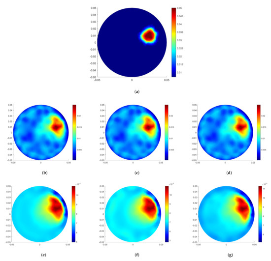
Figure 1. Example 1. (a) True conductivity distribution. (b–d) solution by TV-MMIRGN; (e–g) reconstructions with IRGN at the noise levels 1%, 2%, and 5% from left to right, respectively.

Table 1. Figures of merit for Example 1.

Noise	TV-MMIRGN				IRGN
	${\mathit{RRE}}_1$	${\mathit{RRE}}_2$	SSIM	RE	${\mathit{RRE}}_1$	${\mathit{RRE}}_2$	SSIM	RE
1%	0.211	0.201	0.985	0.015	0.341	0.33	0.94	0.037
2%	0.221	0.305	0.971	0.016	0.35	0.34	0.93	0.041
5%	0.232	0.307	0.961	0.017	0.37	0.39	0.91	0.042

4.2. Example 2

In this second example, we reconstructed one rectangular resistive target with electrical conductivity ${10}^{-8}$ S/m on a regular square domain as shown in Figure 2. We chose a square domain so we could use both versions of the $TV$ operator that we propose. The aim of this numerical example was to test different regularization operators for different types of the domain (circular in Example 1 and square in Example 2) and test for for resistive inclusions [66] (in Example 2) versus conductive inclusions [36] (illustrated in Example 1). We report the visual reconstructions as well as figures of merit to illustrate the reconstruction quality.

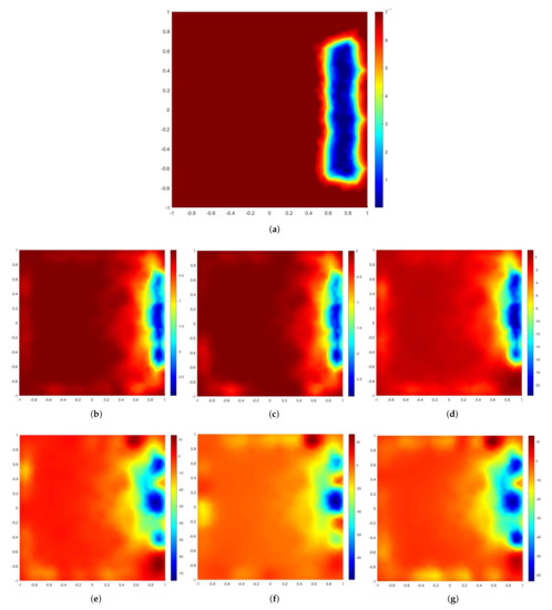
Figure 2. Example 2. (a) True resistive distribution. (b–d) Solution by TV-MMIRGN (second row); (e–g) reconstructions by IRGN (third row) at noise levels 1%, 2%, and 5% from left to right, respectively.

The inclusion is located at the right and side of the domain, close to the boundary. Reconstructions from the TV-MMIRGN are shown in Figure 2b–d. Figure 2e–g show the reconstructions by the IRGN method after iterations using an initial regularization parameter of $\lambda =0.0001$. Reconstruction errors between the two methods are provided in Table 2. This is relatively better posed reconstruction since the inclusion is closer to the boundary than at the center. Therefore, IRGN performed relatively well, but the proposed methods performed better in terms of resolution of the inclusion. This is illustrated in the reconstruction with TV-MMIRGN in this example where we obtained an inclusion of higher quality, and the background is more clear and closer to the true solution shown in Figure 2a.

Table 2. Reconstruction errors from Example 2.

Noise	TV-MMIRGN				IRGN
	${\mathit{RRE}}_1$	${\mathit{RRE}}_2$	SSIM	RE	${\mathit{RRE}}_1$	${\mathit{RRE}}_2$	SSIM	RE
1%	0.141	0.171	0.973	0.018	0.211	0.201	0.985	0.019
2%	0.151	0.175	0.978	0.017	0.221	0.305	0.971	0.019
5%	0.154	0.181	0.983	0.016	0.232	0.307	0.961	0.021

4.3. Example 3

In this last example, we consider a resistive target with electrical conductivity ${10}^{-8}$ and outside the target ${10}^{-3}$ example with 2 inclusions positioned close to the boundary. In this example, we investigate the role of fractional norm p. In particular, we chose values of p to vary from 0.8 to 1.8. The true resistive distribution that was our target of interest is given in Figure 3a. Figure 3b–d represent the reconstructions obtained by FTV-MMIRGN by varying the values of p. Figure 3 shows that choosing smaller values of p allows for us to reconstruct solutions with sharper edges and the reconstructions are of higher quality. Such visual analysis is supported by the figures of merit that are reported in Table 3. In particular, for smaller choice of p we obtain smaller RRE_2 and RE and higher values of SSIM.

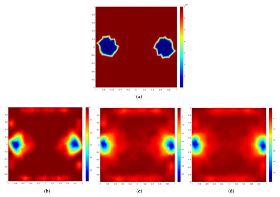
Figure 3. Example 3. (a) True resistive distribution. (b–d) Solution by FTV-MMIRGN (second row) at different values of p, $0.8$, 1, and $1.8$ from left to right, respectively.

Table 3. Figures of merit (relative reconstruction errors for ${\ell }_2$ norm, residual errors, and structural similarity) for Example 3.

p	FTV-MMIRGN
	${\mathrm{RRE}}_2$	SSIM	RE
0.8	0.122	0.932	0.016
1	0.141	0.922	0.017
1.8	0.145	0.919	0.018

5. Conclusions and Future Directions

In this paper, we proposed an iteratively reweighted approach to solve the ${\ell }_p$ regularized EIT to remedy ill-posedness and enhance reconstruction quality by edge enhancement through total variation reconstruction. In EIT imaging, it is common that an anomaly can be modelled as a piecewise constant function over a smooth background. To capture the discontinuity or the sparse nature of the desired solution, we employed a TV-type regularization method to obtain reconstructions with sharp edges. We used a generalized regularization operator $\Theta$. In particular, we examine two special cases, one with the total variation operator defined in the regular rectangular grid that is similar to other imaging modalities (see, e.g., [45,67,68,69]) and in a triangular grid as a special case [70].

Choosing a value of $p\le 1$ causes difficulties with differentiability of the functional to be minimized. Nevertheless, we remedied those difficulties, at least in part, by employing an MM approach that majorizes the functional at each iteration of the linearization and computes a new majorant to be minimized. We investigated the behavior of the minimization function for different values of p. In addition, we compared the approximated solution for two cases, when the regularization operator was identity $\Theta =\mathbf{I}$ and when $\Theta =TV$. When the latter was chosen, the obtained solution was more concentrated with clear and sharp bounds, and high-quality reconstruction. In addition, we compared our approach with the iteratively regularized state-of-the-art Gauss–Newton approach that is very well known for the solution of EIT imaging problems. Our numerical examples illustrate the effectiveness of the obtained solution. Over the past few years, classical and learning techniques have been developed for EIT. The techniques that we propose in this work can be extended to more recent frameworks such as machine learning and neural networks. Such techniques offer robust and automated ways to learn complicated systems through the development and training of a neural network. As future work, we are interested in exploring such techniques to learn regularization parameter $\lambda$ and learn the regularizer or parameter p for the fractional total variation. Moreover, quantifying the uncertainties of the EIT problem is an exciting area of research. We are interested in finding a maximal posterior estimate and in developing efficient sampling methods for uncertainty quantification.

References

- Calderón, A.P. On an inverse boundary value problem. Comput. Appl. Math. 2006, 25, 133–138. [Google Scholar] [CrossRef]
- Boverman, G.; Kao, T.J.; Isaacson, D.; Saulnier, G.J. An implementation of Calderon’s method for 3-D limited-view EIT. IEEE Trans. Med. Imaging 2009, 28, 1073–1082. [Google Scholar] [CrossRef]
- Cherepenin, V.; Karpov, A.; Korjenevsky, A.; Kornienko, V.; Mazaletskaya, A.; Mazourov, D.; Meister, D. A 3D electrical impedance tomography (EIT) system for breast cancer detection. Physiol. Meas. 2001, 22, 9. [Google Scholar] [CrossRef]
- Jang, G.Y.; Ayoub, G.; Kim, Y.E.; Oh, T.I.; Chung, C.R.; Suh, G.Y.; Woo, E.J. Integrated EIT system for functional lung ventilation imaging. Biomed. Eng. Online 2019, 18, 1–18. [Google Scholar] [CrossRef]
- Toivanen, J.; Hänninen, A.; Savolainen, T.; Forss, N.; Kolehmainen, V. Monitoring hemorrhagic strokes using EIT. In Bioimpedance and Spectroscopy; Elsevier: Amsterdam, The Netherlands, 2021; pp. 271–298. [Google Scholar]
- Agnelli, J.P.; Çöl, A.; Lassas, M.; Murthy, R.; Santacesaria, M.; Siltanen, S. Classification of stroke using neural networks in electrical impedance tomography. Inverse Probl. 2020, 36, 115008. [Google Scholar] [CrossRef]
- Patterson, R. Electrical Impedance Tomography: Methods, History, and Applications; Institute of Physics Medical Physics Series; Random Books: New York, NY, USA, 2005. [Google Scholar]
- Bayford, R.H. Bioimpedance tomography (electrical impedance tomography). Annu. Rev. Biomed. Eng. 2006, 8, 63–91. [Google Scholar] [CrossRef]
- Barber, D.C.; Brown, B.H. Applied potential tomography. J. Phys. E Sci. Instrum. 1984, 17, 723. [Google Scholar] [CrossRef]
- Daily, W.; Ramirez, A.; LaBrecque, D.; Nitao, J. Electrical resistivity tomography of vadose water movement. Water Resour. Res. 1992, 28, 1429–1442. [Google Scholar] [CrossRef]
- Stacey, R.; Li, K.; Horne, R.N. Investigating Electrical-Impedance Tomography as a Technique for Real-Time Saturation Monitoring. SPE J. 2009, 14, 135–143. [Google Scholar] [CrossRef][Green Version]
- Isaksen, O.; Dico, A.; Hammer, E.A. A capacitance-based tomography system for interface measurement in separation vessels. Meas. Sci. Technol. 1994, 5, 1262. [Google Scholar] [CrossRef]
- Jin, B.; Maass, P. An analysis of electrical impedance tomography with applications to Tikhonov regularization. ESAIM Control. Optim. Calc. Var. 2012, 18, 1027–1048. [Google Scholar] [CrossRef]
- Jin, B.; Khan, T.; Maass, P. A reconstruction algorithm for electrical impedance tomography based on sparsity regularization. Int. J. Numer. Methods Eng. 2012, 89, 337–353. [Google Scholar] [CrossRef]
- Lionheart, W.R.; Kaipio, J.; McLeod, C.N. Generalized optimal current patterns and electrical safety in EIT. Physiol. Meas. 2001, 22, 85. [Google Scholar] [CrossRef] [PubMed]
- Islam, M.R.; Kiber, M.A. Electrical impedance tomography imaging using gauss-newton algorithm. In Proceedings of the 2014 International Conference on Informatics, Electronics & Vision (ICIEV), Dhaka, Bangladesh, 23–24 May 2014; pp. 1–4. [Google Scholar]
- Hamilton, S.J.; Lionheart, W.; Adler, A. Comparing D-bar and common regularization-based methods for electrical impedance tomography. Physiol. Meas. 2019, 40, 044004. [Google Scholar] [CrossRef] [PubMed]
- Herzberg, W.; Rowe, D.B.; Hauptmann, A.; Hamilton, S.J. Graph Convolutional Networks for Model-Based Learning in Nonlinear Inverse Problems. arXiv 2021, arXiv:2103.15138. [Google Scholar] [CrossRef]
- Kirsch, A.; Grinberg, N. The Factorization Method for Inverse Problems; Oxford University Press: Oxford, UK, 2008; Volume 36. [Google Scholar]
- El Arwadi, T.; Sayah, T. A new regularization of the D-bar method with complex conductivity. Complex Var. Elliptic Equ. 2021, 66, 826–842. [Google Scholar] [CrossRef]
- Mueller, J.L.; Siltanen, S. The d-bar method for electrical impedance tomography—Demystified. Inverse Probl. 2020, 36, 093001. [Google Scholar] [CrossRef]
- Hamilton, S.J.; Hauptmann, A. Deep D-bar: Real-time electrical impedance tomography imaging with deep neural networks. IEEE Trans. Med. Imaging 2018, 37, 2367–2377. [Google Scholar] [CrossRef]
- Kaipio, J.P.; Kolehmainen, V.; Somersalo, E.; Vauhkonen, M. Statistical inversion and Monte Carlo sampling methods in electrical impedance tomography. Inverse Probl. 2000, 16, 1487. [Google Scholar] [CrossRef]
- Sun, X.; Lee, E.; Choi, J.I. Quantification of measurement error effects on conductivity reconstruction in electrical impedance tomography. Inverse Probl. Sci. Eng. 2020, 28, 1669–1693. [Google Scholar] [CrossRef]
- Kaipio, J.; Seppänen, A.; Somersalo, E.; Haario, H. Posterior covariance related optimal current patterns in electrical impedance tomography. Inverse Probl. 2004, 20, 919. [Google Scholar] [CrossRef]
- Nissinen, A.; Heikkinen, L.; Kaipio, J. The Bayesian approximation error approach for electrical impedance tomography—experimental results. Meas. Sci. Technol. 2007, 19, 015501. [Google Scholar] [CrossRef]
- Nissinen, A.; Heikkinen, L.; Kolehmainen, V.; Kaipio, J. Compensation of errors due to discretization, domain truncation and unknown contact impedances in electrical impedance tomography. Meas. Sci. Technol. 2009, 20, 105504. [Google Scholar] [CrossRef]
- Cheng, K.S.; Isaacson, D.; Newell, J.; Gisser, D.G. Electrode models for electric current computed tomography. IEEE Trans. Biomed. Eng. 1989, 36, 918–924. [Google Scholar] [CrossRef]
- Hanke, M.; Harrach, B.; Hyvönen, N. Justification of point electrode models in electrical impedance tomography. Math. Model. Methods Appl. Sci. 2011, 21, 1395–1413. [Google Scholar] [CrossRef]
- Babaeizadeh, S.; Brooks, D.H.; Isaacson, D.; Newell, J.C. Electrode boundary conditions and experimental validation for BEM-based EIT forward and inverse solutions. IEEE Trans. Med. Imaging 2006, 25, 1180–1188. [Google Scholar] [CrossRef]
- Vauhkonen, P.J.; Vauhkonen, M.; Savolainen, T.; Kaipio, J.P. Three-dimensional electrical impedance tomography based on the complete electrode model. IEEE Trans. Biomed. Eng. 1999, 46, 1150–1160. [Google Scholar] [CrossRef]
- Hyvonen, N.; Mustonen, L. Smoothened complete electrode model. SIAM J. Appl. Math. 2017, 77, 2250–2271. [Google Scholar] [CrossRef]
- Dardé, J.; Staboulis, S. Electrode modelling: The effect of contact impedance. ESAIM Math. Model. Numer. Anal. 2016, 50, 415–431. [Google Scholar] [CrossRef]
- Somersalo, E.; Cheney, M.; Isaacson, D. Existence and uniqueness for electrode models for electric current computed tomography. SIAM J. Appl. Math. 1992, 52, 1023–1040. [Google Scholar] [CrossRef]
- Vauhkonen, P.J.; Vauhkonen, M.; Seppänen, A.; Kaipio, J.P. Iterative image reconstruction in three-dimensional electrical impedance tomography. Inverse Probl. Des. Optim. 2004, 1, 152. [Google Scholar]
- Cheney, M.; Isaacson, D.; Newell, J.C. Electrical impedance tomography. SIAM Rev. 1999, 41, 85–101. [Google Scholar] [CrossRef]
- Padilha Leitzke, J.; Zangl, H. A review on electrical impedance tomography spectroscopy. Sensors 2020, 20, 5160. [Google Scholar] [CrossRef] [PubMed]
- Borcea, L. Electrical impedance tomography. Inverse Probl. 2002, 18, R99. [Google Scholar] [CrossRef]
- Tavares, R.S.; Nakadaira Filho, F.A.; Tsuzuki, M.S.; Martins, T.C.; Lima, R.G. Discretization error and the EIT forward problem. IFAC Proc. Vol. 2014, 47, 7535–7540. [Google Scholar] [CrossRef]
- Groetsch, C.W. The Theory of Tikhonov Regularization for Fredholm Equations of the First Kind; Pitman Advanced Pub. Program: Chiyoda, Tokyo, 1984; Volume 105. [Google Scholar]
- Hanke, M.; Hansen, P.C. Regularization methods for large-scale problems. Surv. Math. Ind. 1993, 3, 253–315. [Google Scholar]
- Engl, H.W.; Hanke, M.; Neubauer, A. Regularization of Inverse Problems; Springer Science & Business Media: Berlin/Heidelberg, Germany, 1996; Volume 375. [Google Scholar]
- Lechleiter, A.; Rieder, A. Newton regularizations for impedance tomography: A numerical study. Inverse Probl. 2006, 22, 1967. [Google Scholar] [CrossRef]
- Hansen, P.C. Discrete Inverse Problems: Insight and Algorithms; SIAM: Philadelphia, PA, USA, 2010. [Google Scholar]
- Rudin, L.I.; Osher, S.; Fatemi, E. Nonlinear total variation based noise removal algorithms. Phys. D Nonlinear Phenom. 1992, 60, 259–268. [Google Scholar] [CrossRef]
- Caselles, V.; Chambolle, A.; Novaga, M. Total Variation in Imaging. Handb. Math. Methods Imaging 2015, 1, 1455–1499. [Google Scholar]
- Zhang, Y.; Zhang, W.; Lei, Y.; Zhou, J. Few-view image reconstruction with fractional-order total variation. JOSA A 2014, 31, 981–995. [Google Scholar] [CrossRef]
- Jun, Z.; Zhihui, W. A class of fractional-order multi-scale variational models and alternating projection algorithm for image denoising. Appl. Math. Model. 2011, 35, 2516–2528. [Google Scholar] [CrossRef]
- Beck, A.; Teboulle, M. Fast gradient-based algorithms for constrained total variation image denoising and deblurring problems. IEEE Trans. Image Process. 2009, 18, 2419–2434. [Google Scholar] [CrossRef] [PubMed]
- Björk, Å. Numerical Methods for Least Squares Problems; Society for Industrial and Applied Mathematics: Philadelphia, PA, USA, 1996; p. 147. [Google Scholar]
- Vauhkonen, P. Image Reconstruction in Three-Dimensional Electrical Impedance Tomography (Kolmedimensionaalinen Kuvantaminen Impedanssitomografiassa); Kuopion Yliopisto: Kuopio, Finland, 2004. [Google Scholar]
- Pes, F.; Rodriguez, G. A doubly relaxed minimal-norm Gauss–Newton method for underdetermined nonlinear least-squares problems. Appl. Numer. Math. 2022, 171, 233–248. [Google Scholar] [CrossRef]
- Wohlberg, B.; Rodriguez, P. An iteratively reweighted norm algorithm for minimization of total variation functionals. IEEE Signal Process. Lett. 2007, 14, 948–951. [Google Scholar] [CrossRef]
- Bube, K.P.; Langan, R.T. Hybrid ℓ 1/ℓ 2 minimization with applications to tomography. Geophysics 1997, 62, 1183–1195. [Google Scholar] [CrossRef]
- Beaton, A.E.; Tukey, J.W. The fitting of power series, meaning polynomials, illustrated on band-spectroscopic data. Technometrics 1974, 16, 147–185. [Google Scholar] [CrossRef]
- Darbon, J.; Sigelle, M. Image restoration with discrete constrained total variation part I: Fast and exact optimization. J. Math. Imaging Vis. 2006, 26, 261–276. [Google Scholar] [CrossRef]
- Lange, K. MM Optimization Algorithms; SIAM: Philadelphia, PA, USA, 2016. [Google Scholar]
- Romano, D.; Pisa, S.; Piuzzi, E. Implementation of the Newton-Raphson and admittance methods for EIT. Int. J. Bioelectromagn. 2010, 12, 12–20. [Google Scholar]
- Tan, R.H.; Rossa, C. Electrical Impedance Tomography using Differential Evolution integrated with a Modified Newton Raphson Algorithm. In Proceedings of the 2020 IEEE International Conference on Systems, Man, and Cybernetics (SMC), Toronto, ON, Canada, 11–14 October 2020; pp. 2528–2534. [Google Scholar]
- MacNeal, B.E.; Brauer, J.R. Electrical circuits and finite element field models: A general approach. In Finite Elements, Electromagnetics and Design; Elsevier: Amsterdam, The Netherlands, 1995; pp. 179–199. [Google Scholar]
- Spyrakos, C.C. Finite Element Modeling; West Virginia Univ. Press: Morgantown, WV, USA, 1994. [Google Scholar]
- Kaipio, J.; Somersalo, E. Statistical inverse problems: Discretization, model reduction and inverse crimes. J. Comput. Appl. Math. 2007, 198, 493–504. [Google Scholar] [CrossRef]
- Nocedal, J.; Wright, S.J. Numerical Optimization; Springer: Berlin/Heidelberg, Germany, 2006. [Google Scholar]
- Lanza, A.; Morigi, S.; Reichel, L.; Sgallari, F. A generalized Krylov subspace method for ℓp − ℓq minimization. SIAM J. Sci. Comput. 2015, 37, S30–S50. [Google Scholar] [CrossRef]
- Huang, G.; Lanza, A.; Morigi, S.; Reichel, L.; Sgallari, F. Majorization–minimization generalized Krylov subspace methods for ℓp − ℓq optimization applied to image restoration. BIT Numer. Math. 2017, 57, 351–378. [Google Scholar] [CrossRef]
- Wu, C.; Hutton, M.; Soleimani, M. Limited angle electrical resistance tomography in wastewater monitoring. Sensors 2020, 20, 1899. [Google Scholar] [CrossRef] [PubMed]
- Yang, X.; Yao, S.; Lim, K.P.; Lin, X.; Rahardja, S.; Pan, F. An adaptive edge-preserving artifacts removal filter for video post-processing. In Proceedings of the 2005 IEEE International Symposium on Circuits and Systems, Kobe, Japan, 23–26 May 2005; pp. 4939–4942. [Google Scholar]
- Vogel, C.R.; Chan, T.F.; Plemmons, R.J. Fast algorithms for phase-diversity-based blind deconvolution. Adaptive Optical System Technologies. Int. Soc. Opt. Photonics 1998, 3353, 994–1005. [Google Scholar]
- Cui, B.; Ma, X.; Xie, X.; Ren, G.; Ma, Y. Classification of visible and infrared hyperspectral images based on image segmentation and edge-preserving filtering. Infrared Phys. Technol. 2017, 81, 79–88. [Google Scholar] [CrossRef]
- Gong, B.; Schullcke, B.; Krueger-Ziolek, S.; Zhang, F.; Mueller-Lisse, U.; Moeller, K. Higher order total variation regularization for EIT reconstruction. Med. Biol. Eng. Comput. 2018, 56, 1367–1378. [Google Scholar] [CrossRef] [PubMed]
Publisher’s Note: MDPI stays neutral with regard to jurisdictional claims in published maps and institutional affiliations. |
© 2022 by the authors. Licensee MDPI, Basel, Switzerland. This article is an open access article distributed under the terms and conditions of the Creative Commons Attribution (CC BY) license (https://creativecommons.org/licenses/by/4.0/).