Design of an LMI-Based Fuzzy Fast Terminal Sliding Mode Control Approach for Uncertain MIMO Systems

Abstract

This paper proposes a linear matrix inequality (LMI)-based fuzzy fast terminal sliding mode control (FFTSM) approach for a multi-input multi-output (MIMO) system. This design aims to achieve the finite-time convergence of system trajectories to their desired values, while at the same time eliminating the chattering problem. Finite-time stability is proven using the Lyapunov theory and the control parameters are obtained using the LMI approach. The fuzzy logic approach is considered to fine tune the controller parameters and reduce the tracking error and control signal amplitude. The performance of the proposed approach is assessed using a simulation study of a direct current (DC) motor. The obtained results confirm the effectiveness of the proposed control design. Simplicity of the design, robustness, finite-time convergence, and chattering-free dynamics are among the features of the proposed approach.

1. Introduction

Controlling uncertain systems is one of the most challenging problems in control theory. Owing to its effectiveness, simplicity, disturbance rejection capability, insensitivity to parameter variations and ease of implementation, sliding mode control (SMC) has been widely considered in controlling uncertain nonlinear systems [1]. It has been successfully implemented in various applications such as power grids, electric motors, automotive systems, communication networks, and robotic systems, and so on [2]. SMC is achieved following two stages: a reaching phase and a switching phase [3]. In the reaching phase, a control signal steers the system states to a sliding surface, and in the switching phase, a sliding surface is defined so that the system states remain on that surface [4,5]. Standard SMC, however, suffers from two major drawbacks: (1) convergence of the system states to the equilibrium point in finite time is not guaranteed; and (2) the chattering phenomena resulting from the discontinuous control. Terminal Sliding Mode Control (TSMC) was developed to achieve finite-time convergence in single input single output (SISO) and MIMO systems [6,7,8]. In TSMC, a power fraction term is used on the sliding surface to ensure finite-time convergence [9]. The nonlinear sliding surface in TSMC ramps up the control input to speed up the convergence [10]. The idea of fast terminal sliding mode was introduced in [11], to ensure faster transient convergence rates and robustness to uncertainties. In [12], a new structure was introduced for FTSM. The finite-time stability in chaotic systems was investigated by the FTSM method in [13].

The authors in [14] proposed a recursive FTSM that archives finite-time tracking and removes the singularity problem in the control phase. An FTSM-based fault tolerant control was proposed in [15], and was shown to achieve a fast convergence speed. By combining the TSMC and backstepping method, a controller was designed in [16] for industrial robotics to achieve finite-time convergence and reduced oscillations. In [16], a newly modified fast integral terminal sliding state control law was designed for the spacecraft formation system. External disturbances were estimated in that approach using a reduced-order perturbation observer. In [17], an LMI-based second-order FTSM was proposed for chaotic systems. The use of FTSM for multi-input multi-output (MIMO) systems with uncertainties and chaos was carried out in [18]. A TSM-based nonlinear sliding surface was proposed in [19] for MIMO systems. The position of the state error bound was expressed in that approach using LMIs. An FTSMC approach was considered for the multi-input multi-output twin-rotor system in [20]. In [21], by using the fixed-time disturbance observer, the tracking control of aircraft with external disturbances and measuring noises was investigated; however, the suggested method [21] did not provide a law to adjust the switching control gains and improve the system’s dynamic response. The study reported in [22] showed that combining the FTSMC with a fuzzy logic approach to adjust the sliding surface and switching control gains can further improve the system’s dynamic response. A PSO optimized super-twisting finite-time SMC technique was designed in [23] for PMSM systems with external disturbances. An adaptive finite-time SMC approach was introduced in [24] for a class of uncertain systems with external disturbances and input saturation. In [25], by using TSM and fuzzy, an adaptive controller was designed for MIMO systems, and the performance of this strategy was evaluated through the control of ankle and knee movement and a two-link rigid robotic manipulator. A design of a MIMO fuzzy terminal sliding mode controller was proposed in [26] for a manipulator robotic. An intelligent nonsingular terminal sliding mode approach with type 2 fuzzy logic control was proposed in [27] for the wind turbine system. In [28], a fuzzy adaptive fixed time SMC method with state-observer was designed for a class of uncertain systems such as ship course and robotic manipulators. By means of the known bounds of membership functions in interval type-2 fuzzy models, the SMC and fuzzy observer methods are addressed in [29] to guarantee the reachability of the SMC dynamics. In [30], the SMC approach was presented for the discrete-time interval type-2 fuzzy singularly disturbed system where the optimization algorithm reduces the convergence domain around the sliding surface.

To the best of the authors’ knowledge, most finite-time controllers, such as FTSM and TSM, have been applied to single-input, single-output (SISO) systems. This paper proposes an LMI-based FFTSM control design for MIMO uncertain systems. The main contributions of this paper are as follows:

• A robust approach that yields faster finite-time convergence of the system states to the equilibrium, while it ensures chattering-free dynamics, even in the presence of uncertainties.
• An approach that combines FTSMC with fuzzy logic to adjust the sliding surface and switching control gains and further improve the system’s dynamic response.
• A FTSC approach in which control parameters are determined using the LMI approach.

The rest of the paper is organized as follows. Section 2 provides the problem formulation. Stability analysis and control law are described in Section 3 and Section 4. The simulation results are reported in Section 5. Finally, conclusions are provided in Section 6.

2. Problem Statement and Assumption

Consider the following MIMO system with uncertainties [31]:

$$\begin{gathered} {\dot{x}}_1=A_{11} x_1+A_{12} x_2+f_u \left(t,x\right) \\ {\dot{x}}_2=A_{21} x_1+A_{22} x_2+B_{2}u+f_m \left(t,x,u\right) \\ y=Cx \end{gathered}$$

(1)

where $x={\left[ x_1 x_2 \right]}^T$ are the state vector, and $x_1\in R^{n-m},x_2\in R^{m\times m}$, $y$ is output and $y\in R^{n-m}$, $f_u \left(t, x\right)\in R^{n-m}$ and $f_m \left(t,x,u\right)\in R^m$ are known as the system uncertainties, $B_2$ is $m\times m$ matrix and $C$ is $P\times n$ matrix, $A=\left[\begin{array}{cc}{A}_{11}& A_{12}\\ A_{21}& A_{22}\end{array}\right]$ is a constant matrix; $A_{11}\in R^{\left(n-m\right)\times \left(n-m\right)}$, $A_{12}\in R^{\left(n-m\right)\times m}$, $A_{21}\in R^{m\times \left(n-m\right)}$ and $A_{22}\in R^{m\times m}$ are constant sub-matrices; $f_m \left(t,x,u\right)$ and $f_u \left(t,x\right)$ denote the matched and mismatched uncertainties. These latter satisfy the following inequalities:

$$\Vert f_u \left(t,x\right)\Vert \le L_u$$

(2)

$$\Vert f_m \left(t,x,u\right)\Vert \le L_m$$

(3)

where $L_u$ and $L_m$ are the upper bound of $f_{u }, f_m$.

The sliding surface for system (1) is defined as follows:

$$S\left(e\right)=\mathsf{\Gamma }\left(e\right)$$

(4)

$\mathsf{\Gamma }$ in the above equation is defined as $\mathsf{\Gamma }=\left[F G\right]$. $F$ $\left(m\times m\right)$ and $G$ $\left(m\times \left(n-m\right)\right)$ are gain matrices. $e\left(t\right)={\left[e_1\left(t\right) e_2\left(t\right) \right]}^T$ is the error signal:

$$e_1=x_1-x_{d1}$$

(5)

$$e_2=x_2-x_{d2}$$

(6)

where $x_d={\left[x_{d1} x_{d2} \right]}^T$ represents the reference trajectory. Using Equation (4), the FTSMC surface [10] is defined by

$$\sigma \left(e\right)=S\left(e\right)+\dot{S}\left(e\right)+S{\left(e\right)}^{\raisebox{1ex}{$p$}\!\left/ \!\raisebox{-1ex}{$q$}\right.}$$

(7)

where $\raisebox{1ex}{$p$}\!\left/ \!\raisebox{-1ex}{$q$}\right.$ is an odd positive constant, such that $\frac{1}{2}<\raisebox{1ex}{$p$}\!\left/ \!\raisebox{-1ex}{$q$}\right.<1$. When the sliding surface reaches the equilibrium point, $S\left(e\right)=0$, Equation (4) becomes:

$$e_2=-G^{-1}F{e}_1$$

(8)

Equations (1), (5) and (8) are used to obtain:

$$\begin{gathered} {\dot{e}}_1={\dot{x}}_1-{\dot{x}}_{d1}=A_{11}{e}_1-A_{12} G^{-1}F{e}_1+A_{11}{x}_{d1}+A_{12}{x}_{d2}-{\dot{x}}_{d1}+ \\ {f}_u\left(t,x\right)=\left(A_{11}-A_{12}{G}^{-1}F\right)e_1+A_{11}{x}_{d1}+A_{12}{x}_{d2}-{\dot{x}}_{d1}+f_u\left(t,x\right) \end{gathered}$$

(9)

Note 1: The nonlinear functions $f_u\left(x,t\right)$ and $f_m\left(t,x,u\right)$ are assumed to be differentiable.

Assumption 1.

The$u_d$for reference trajectory$x_d$is defined as follow:

$${\dot{x}}_d=A{x}_d+B{u}_d$$

(10)

where${\dot{x}}_d, x_d$ and $u_d$ are assumed to be smooth vector functions. The vector $x_d$ must be generated in such a way that it is consistent with the dynamics of (A, B). Equation (10) can be rewritten as:

$${\dot{x}}_{d1}=A_{11}{x}_{d1}+A_{12}{x}_{d2}$$

(11)

$${\dot{x}}_{d2}=A_{21}{x}_{d1}+A_{22}{x}_{d2}+B_2{u}_d$$

(12)

By substituting (11) into (9), the term $\dot{e_1}$ is re-written as:

$$\dot{e_1}=\left(A_{11}-A_{12}{G}^{-1}\right)e_1+f_u\left(t,x\right)$$

(13)

Lemma 1.

Consider a positive definite continuously Lyapunov function candidate$V\left(t\right)$. The derivative of$V\left(t\right)$must have the fallowing conditions:

$$\begin{gathered} \dot{V}\left(t\right)\le -\alpha V\left(t\right)-\beta V^{\raisebox{1ex}{$p$}\!\left/ \!\raisebox{-1ex}{$q$}\right.}\left(t\right)\hspace{1em}\hspace{1em}\forall t\ge t_0 \\ V\left(t_0\right)\ge 0 \end{gathered}$$

(14)

where$\alpha and \beta$are positive constants,$\raisebox{1ex}{$p$}\!\left/ \!\raisebox{-1ex}{$q$}\right.$chosen as an odd number and it is$0<\raisebox{1ex}{$p$}\!\left/ \!\raisebox{-1ex}{$q$}\right.<1$.

The above equation is re-written as follows:

$$V^{-\raisebox{1ex}{$p$}\!\left/ \!\raisebox{-1ex}{$q$}\right.}\left(t\right)\dot{V}\left(t\right)\le -\alpha V^{1-\raisebox{1ex}{$p$}\!\left/ \!\raisebox{-1ex}{$q$}\right.}\left(t\right)-\beta$$

(15)

and also:

$$dt\le -\frac{V^{-\raisebox{1ex}{$p$}\!\left/ \!\raisebox{-1ex}{$q$}\right.}\left(t\right)}{\alpha V^{1-\raisebox{1ex}{$p$}\!\left/ \!\raisebox{-1ex}{$q$}\right.}\left(t\right)+\beta }dV\left(t\right)$$

(16)

Integrating the above expression yields:

$$dt\le -\frac{V^{-\raisebox{1ex}{$p$}\!\left/ \!\raisebox{-1ex}{$q$}\right.}\left(t\right)}{\alpha V^{1-\raisebox{1ex}{$p$}\!\left/ \!\raisebox{-1ex}{$q$}\right.}\left(t\right)+\beta }dV\left(t\right)$$

(17)

$$t_r-t_0\le {{\displaystyle \int }}_{V\left(t_0\right)}^0\frac{V^{-\raisebox{1ex}{$p$}\!\left/ \!\raisebox{-1ex}{$q$}\right.}\left(t\right)}{\alpha V^{1-\raisebox{1ex}{$p$}\!\left/ \!\raisebox{-1ex}{$q$}\right.}\left(t\right)+\beta }dV\left(t\right)=-\frac{1}{\alpha \left(1-\raisebox{1ex}{$p$}\!\left/ \!\raisebox{-1ex}{$q$}\right.\right)}[ln\beta -ln\left(\alpha V^{1-\raisebox{1ex}{$p$}\!\left/ \!\raisebox{-1ex}{$q$}\right.}\left(t_0\right)\right]$$

(18)

Lyapunov’s function converges to zero the finite time $t_r$, defined by:

$$t_r=t_0+\frac{1}{\alpha \left(1-\raisebox{1ex}{$p$}\!\left/ \!\raisebox{-1ex}{$q$}\right.\right)}ln\frac{\alpha V^{1-\raisebox{1ex}{$p$}\!\left/ \!\raisebox{-1ex}{$q$}\right.}\left(t\right)+\beta }{\beta }$$

(19)

3. Main Results

Theorem 1.

Consider Equation (13). Assuming$\Vert f_u \left(t,x\right)\Vert \le L_u$and${\Vert e}_1\Vert \ge r$, where$r$and$L_u$are positive constants. If there exist matrices such as$X>0,$ $W>0$, $G>0,$ $Q>0$. In addition,${\mu }_1>0$and${\mu }_2>0$are two scalar values. $y$with the right dimensions, the LMI will be [17]:

$$\left[\begin{array}{cc}{A}_{11}X+X{A}_{11}^T-A_{12}Y-Y^T{A}_{12}^T+Q& X\\ X& -W\end{array}\right]<0$$

(20)

$${\mu }_1{I}_{n-m}-Q<0$$

(21)

$${\mu }_2{I}_{n-m}-W<0$$

(22)

$${\mu }_1-\frac{L_u^2}{r^2}{\mu }_2>0$$

(23)

Then consider a positive definite matrix such that $P=X^{-1}$ and $F=GY{X}^{-1}$ in (4). System (13) will be asymptotically bounded by ${\Vert e}_1\Vert \ge r$.

Select the candidate Lyapunov function as:

$$V_1\left(e_1\right)=e_1^{T}P{e}_{1 }$$

(24)

Differentiating the above equation and substituting (13) in it yields:

$${\dot{V}}_1\left(e_1\right)=e_1^{T}P{\dot{e}}_1+{\dot{e}}_1^{T}P{e}_{1 }=e_1^T(P\left(A_{11}-A_{12}{G}^{-1}F\right)+\left(A_{11}-A_{12}{G}^{-1}F{)}^{T}P\right)e_{1 }+e_1^{T}P f_u\left(t,x\right)+f_u^T\left(t, x\right)P{e}_{1 }$$

(25)

The following inequality can be used for the last term (25) and (24):

$$e_1^{T}P f_u\left(t,x\right)+f_u^T\left(t, x\right)P{e}_{1 }\le e_1^{T}PQP{e}_{1 }+f_u^T\left(t, x\right)Q^{-1}{f}_u\left(t, x\right)\le e_1^{T}PQP{e}_{1 }+l_u^2{\lambda }_{max}\left(Q^{-1}\right)$$

(26)

${\lambda }_{max}\left(Q^{-1}\right)$ is the maximum specific value of $Q^{-1}$. The $Q-matrix$ is positive definite. The above two equations can be written using the following inequality:

$$\frac{e_1^T{e}_1}{r^2}\ge 1$$

(27)

By the condition ${\Vert e}_1\Vert \ge r$, the following inequality is achieved:

$${\dot{V}}_1\left(e_1\right)\le e_1^T\left(P\left(A_{11}-A_{12}{G}^{-1}F\right)+\left(A_{11}-A_{12}{G}^{-1}F{)}^{T}P\right)+PQP\right)e_{1 }+ l_u^2{\lambda }_{max}\left(Q^{-1}\right)$$

(28)

By using (26) and (28), the following equation is obtained:

$${\dot{V}}_1\left(e_1\right)\le e_1^T\left(P\left(A_{11}-A_{12}{G}^{-1}F\right)+\left(A_{11}-A_{12}{G}^{-1}F{)}^{T}P\right)+PQP\right)+\frac{l_u^2}{r^2}{\lambda }_{max}\left(Q^{-1}\right)I_{n-m})e_1$$

(29)

Now, using the following equation:

$$P\left(A_{11}-A_{12}{G}^{-1}F\right)+\left(A_{11}-A_{12}{G}^{-1}F{)}^{T}P\right)+PQP\le -W^{-1}$$

(30)

We can simplify (29) as:

$${\dot{V}}_1\left(e_1\right)\le -(({\lambda }_{min}(W^{-1})-\frac{l_u^2}{r^2}{\lambda }_{max}(Q^{-1})){{\Vert e}_1\Vert }^2$$

(31)

where ${\lambda }_{min}\left(W^{-1}\right)$ is the minimum specific value of $W^{-1}.$ If

$${\alpha }_1=\frac{{\lambda }_{min}\left(W^{-1}\right)-\frac{l_u^2}{r^2}{\lambda }_{max}\left(Q^{-1}\right)}{{\lambda }_{max}\left(P\right)}$$

(32)

Equation (31) can be written as:

$${\dot{V}}_1\left(e_1\right)\le -{\alpha }_1{V}_1\left(e_1\right)$$

(33)

Since ${\alpha }_1\ge 0$, we have:

$${\mu }_1<{\lambda }_{min}\left(Q\right)$$

(34)

$${\mu }_2>{\lambda }_{max}\left(W\right)$$

(35)

Given the above equations, the following inequality is obtained:

$${\lambda }_{min}\left(Q\right)-\frac{l_u^2}{r^2}{\lambda }_{max}\left(W\right)>0$$

(36)

If $X=P^{-1}$, pre and post multiplying (30) by X yields:

$$A_{11}\mathrm{X}-A_{12}{G}^{-1}FX+X{(A_{11}-A_{12}{G}^{-1}F)}^T+Q\le -X{W}^{-1}X$$

(37)

Considering $Y=G^{-1}FX$ and Schur compliment [32], the LMI condition is realized.

Theorem 2.

Consider the nonlinear system (1) and the sliding surface (7). Assume that F and G are found via LMI. If the control signal is defined as follows, then the states will reach the sliding surface with any initial condition in the finite time:

$$\dot{u}={\left(G{B}_2\right)}^{-1}\left\{k-\left(\raisebox{1ex}{$p$}\!\left/ \!\raisebox{-1ex}{$q$}\right.diag\left(s^{\raisebox{1ex}{$p$}\!\left/ \!\raisebox{-1ex}{$q$}\right.-1}\right)+I_m\right)G{B}_2-\left(F{A}_{12}+G{A}_{22}\right)B_2)u\right\}$$

(38)

where the value of$k$is determined as follows:

$$\begin{gathered} k=-((\raisebox{1ex}{$p$}\!\left/ \!\raisebox{-1ex}{$q$}\right. diag\left(s^{\raisebox{1ex}{$p$}\!\left/ \!\raisebox{-1ex}{$q$}\right.-1}\right)+I_m)\left[ \mathsf{\Gamma }Ae+G{B}_{2}f\left(x\right)\right]+\mathsf{\Gamma }{A}^{2}e+G{B}_2\dot{f}\left(x\right)+ \\ \left(F{A}_{12}+G{A}_{22}\right)B_{2}f\left(x\right)+\mathsf{\Pi }sign\left(\sigma \right)+\gamma \sigma +\phi sign\left(\sigma \right)\mid \sigma {\mid }^{\raisebox{1ex}{$p$}\!\left/ \!\raisebox{-1ex}{$q$}\right.}) \end{gathered}$$

(39)

where$p$and$q$should be selected as positive odd numbers with$q>p>0$to avoid the singularity problem in the controller. The terms$\phi$and$\gamma$are positive coefficients and$\mathsf{\Pi }$is upper bound of uncertainties.

Candidate Lyapunov function as follows:

$$V_2\left(\sigma \right)=\frac{1}{2}{\sigma }^T\sigma$$

(40)

The term ${\dot{e}}_2$ is obtained by the same procedure as ${\dot{e}}_1$ as follows:

$${\dot{e}}_2=A_{21}{e}_1+A_{22}{e}_2+B_2\left(u+f\left(x\right)\right)+f_m \left(t,x,u\right)$$

(41)

The first-order derivative of the sliding surface is as follows:

$$\dot{s}\left(e\right)=F\left(A_{11}{e}_1+A_{12}{e}_2+f_u \left(t,x\right)\right)+G(A_{21}{e}_1+A_{22}{e}_2+B_2\left(u+f\left(x\right)\right)+f_m \left(t,x,u\right)$$

(42)

and the second-order derivative of the sliding surface is introduced as follows:

$$\begin{array}{c}\ddot{s}\left(e\right)=\left(F{A}_{12}+G{A}_{22}\right)(A_{21}{e}_1+A_{22}{e}_2+B_2\left(u+f\left(x\right)\right)+f_m \left(t,x,u\right)+\hfill \\ \left(F{A}_{11}+G{A}_{21}\right)\left(A_{11}{e}_1+A_{12}{e}_2+f_u \left(t,x\right)\right)+G{B}_2\left(\dot{u}+\dot{f}\left(x\right)\right)+F{\dot{f}}_u \left(t,x\right)+\hfill \\ G{\dot{f}}_m\left(t,x,u\right)\hfill \end{array}$$

(43)

Deriving (40) yields:

$${\dot{V}}_2\left(\sigma \right)={\sigma }^T\dot{\sigma }={\sigma }^T(\left(\raisebox{1ex}{$p$}\!\left/ \!\raisebox{-1ex}{$q$}\right.diag\left(s^{\raisebox{1ex}{$p$}\!\left/ \!\raisebox{-1ex}{$q$}\right.-1}\right)+I_m\right)\dot{s}+\ddot{s}$$

(44)

Equation (44) can be simplified as follows:

$$\begin{array}{c}{\dot{V}}_2\left(\sigma \right)={\sigma }^T\{\left(\raisebox{1ex}{$p$}\!\left/ \!\raisebox{-1ex}{$q$}\right.diag\left(s^{\raisebox{1ex}{$p$}\!\left/ \!\raisebox{-1ex}{$q$}\right.-1}\right)+I_m\right)\left[F(A_{11}{e}_1+A_{12}{e}_2+f_u \left(t,x\right)\right]+G(A_{21}{e}_1+A_{22}{e}_2+\hfill \\ B_{2}f\left(x\right)+f_m (t,x,u))]+F{\dot{f}}_u \left(t,x\right)+\left(F{A}_{12}+G{A}_{22}\right)(A_{21}{e}_1+A_{22}{e}_2+B_{2}f\left(x\right)+f_m (t,x,u))+\hfill \\ G{\dot{f}}_m \left(t,x,u\right)+\left(F{A}_{11}+G{A}_{21}\right)\left(A_{11}{e}_1+A_{12}{e}_2+f_u \left(t,x\right)\right)+G{B}_2\dot{f}\left(x\right)+k\}\hfill \end{array}$$

(45)

Substituting $k$ in (45), yields:

$$\begin{array}{c}{\dot{V}}_2\left(\sigma \right)=-{\sigma }^T\phi sign\left(\sigma \right){\left|\sigma \right|}^{\raisebox{1ex}{$p$}\!\left/ \!\raisebox{-1ex}{$q$}\right.}-{\sigma }^T\gamma \sigma -{\sigma }^T\mathsf{\Pi }sign\left(\sigma \right)+{\sigma }^T\left(\raisebox{1ex}{$p$}\!\left/ \!\raisebox{-1ex}{$q$}\right.diag\left(s^{\raisebox{1ex}{$p$}\!\left/ \!\raisebox{-1ex}{$q$}\right.-1}\right)+I_m\right)+\hfill \\ {\sigma }^T\mathsf{\Gamma }\left(A{f}_{u, m}+{\dot{f}}_{u,m}\right)\hfill \end{array}$$

(46)

where ${\alpha }_2=2{\lambda }_{min}\left(\gamma \right)>0$ and ${\beta }_2=2^{\frac{\left(\frac{p}{q}+1\right)}{2}{\lambda }_{min}}\left(\phi \right)>0$

Equation (46) can be resulted as:

$${\dot{V}}_2\left(\sigma \right)\le -{\lambda }_{min}\left(\gamma \right){\Vert \sigma \Vert }^2-{\lambda }_{min}\left(\phi \right){\Vert \sigma \Vert }^{\raisebox{1ex}{$p$}\!\left/ \!\raisebox{-1ex}{$q$}\right.+1}=-{\alpha }_2{V}_2\left(\sigma \right)-{\beta }_2{V}_2^{\frac{\raisebox{1ex}{$p$}\!\left/ \!\raisebox{-1ex}{$q$}\right.+1}{2}}$$

(47)

and $\frac{\raisebox{1ex}{$p$}\!\left/ \!\raisebox{-1ex}{$q$}\right.+1}{2}<1$.

The states will reach the surface in the finite time $t_r$, defined by:

$$t_r=\frac{1}{{\alpha }_2\left(1-\frac{\raisebox{1ex}{$p$}\!\left/ \!\raisebox{-1ex}{$q$}\right.+1}{2}\right)}ln\frac{{\alpha }_2{V}_2{(\sigma \left(t_0\right))}^{1-\frac{\raisebox{1ex}{$p$}\!\left/ \!\raisebox{-1ex}{$q$}\right.+1}{2}}+{\beta }_2}{{\beta }_2}$$

(48)

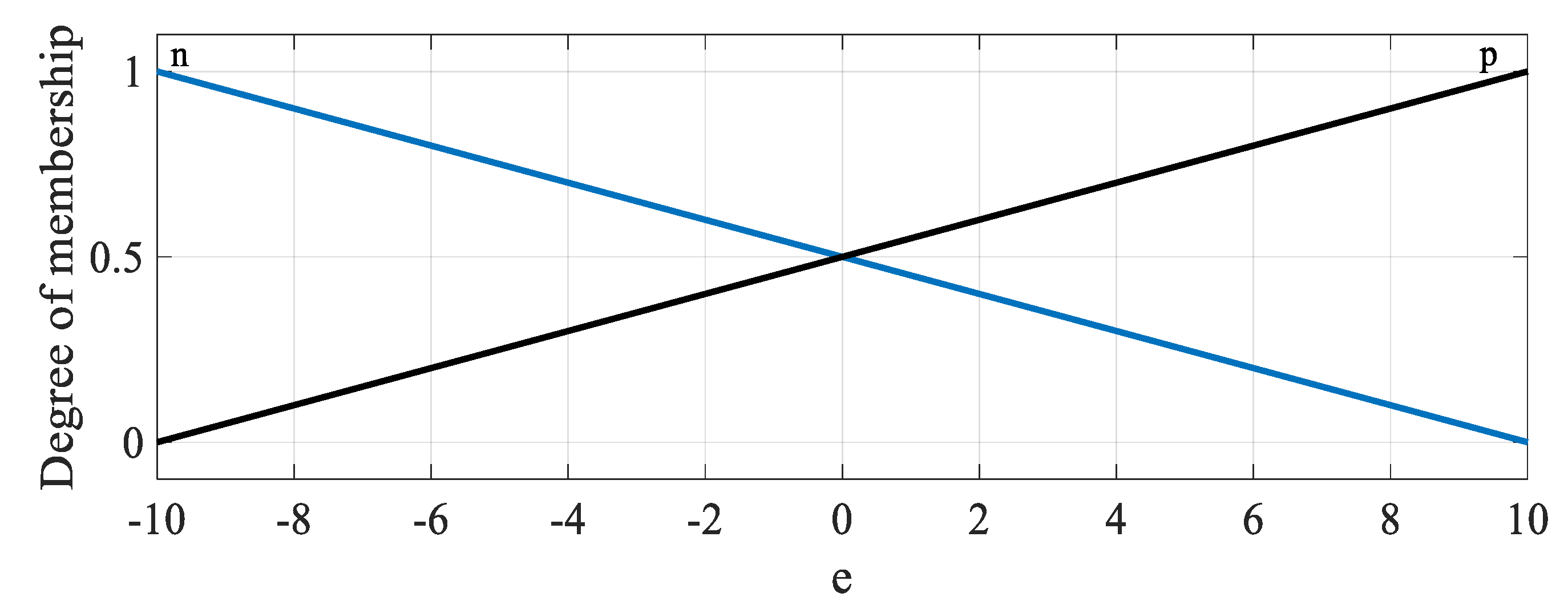
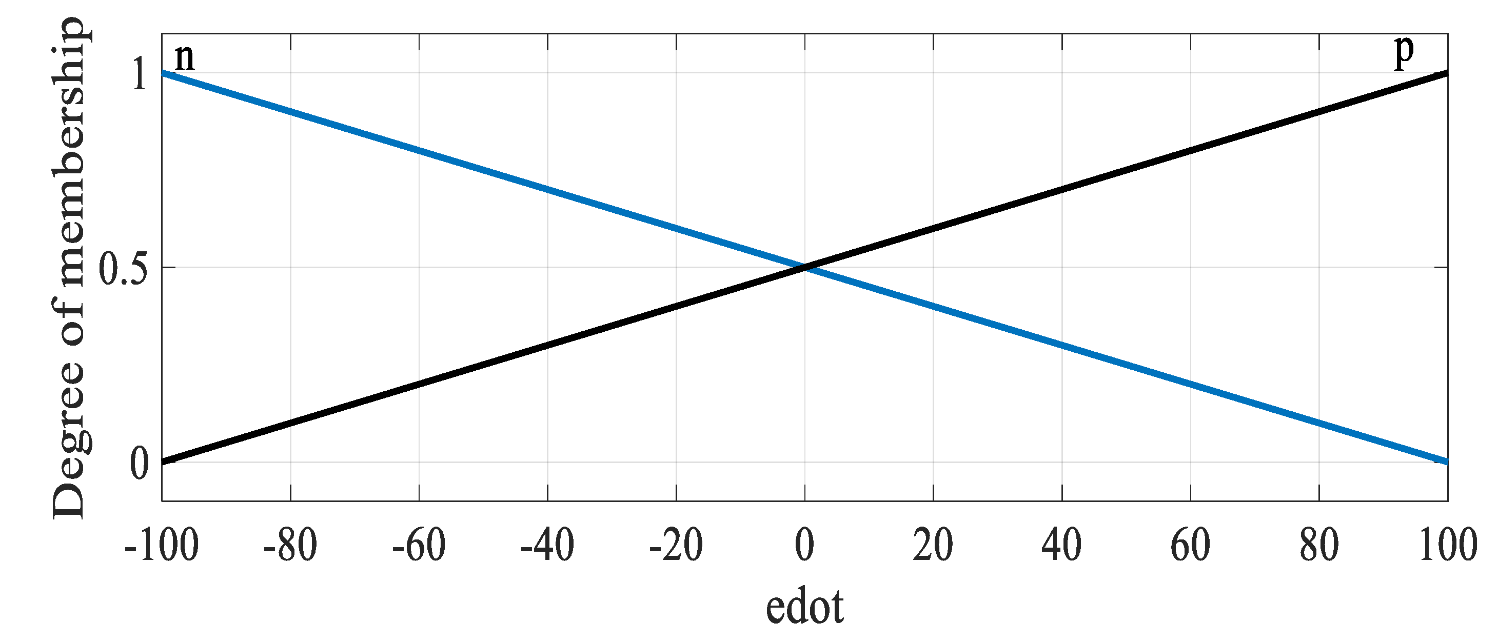
4. Fuzzy Fast Terminal Sliding Mode

To improve the results, a fuzzy control can be integrated with the FTSM control. This method can (1) eliminated chattering, (2) reduce the amplitude of the control signal, and (3) reduce the error [33,34]. Selection of the fuzzy rules is the first problem to be resolved. Usually, the sliding surface $(s$), time-derivative of sliding surface ($\dot{s}$), error signal ($e)$ and its time-derivative ($\dot{e}$) are selected as Fuzzy inputs [35,36]. For the fuzzy input, the triangular membership functions (trimf) are considered, and for the fuzzy output, the singletons membership functions are used. It is clear that the output should track the reference signal. Given that the output is lower or higher than the reference path and based on the definition of the error signals (5) and (6), the negative and positive signs of the error signal are determined. Furthermore, the sign of the function $\dot{e}$ is related to the slope of the output diagram. The error signal and its time-derivative are used in the sliding surface (7). Hence, their sign plays an important role in the determination of the sign of the sliding surface. The fuzzy rules are chosen so that if the output deviates from the reference path, it can be brought closer for accurate tracking purposes.

In this work, the error $e$ and its derivative $\dot{e}$ are selected as a Fuzzy input and the sliding surface $s$ as the output, where N, P and Z stand for negative, positive and zero in fuzzy language [37]. The fuzzy rules are written in

Table 1. Fuzzy rules.

$\mathit{s}.$	$\dot{\mathit{e}}$	$\mathit{e}$
$Z$	$N$	$P$
$N$	$N$	$N$
$P$	$P$	$P$
$Z$	$P$	$N$

. The graph of membership function is given in the simulation results section.

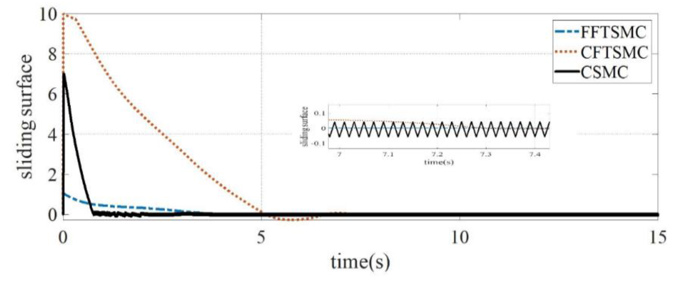
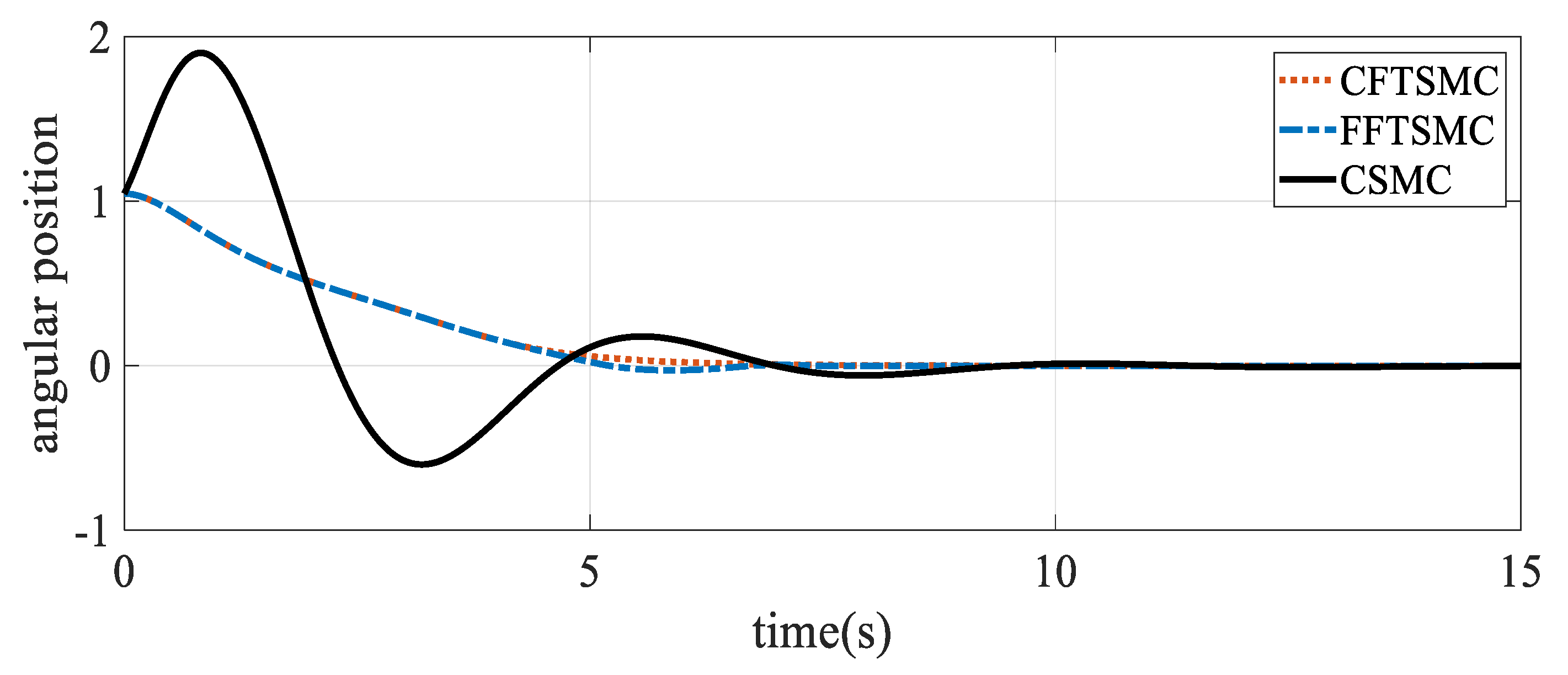
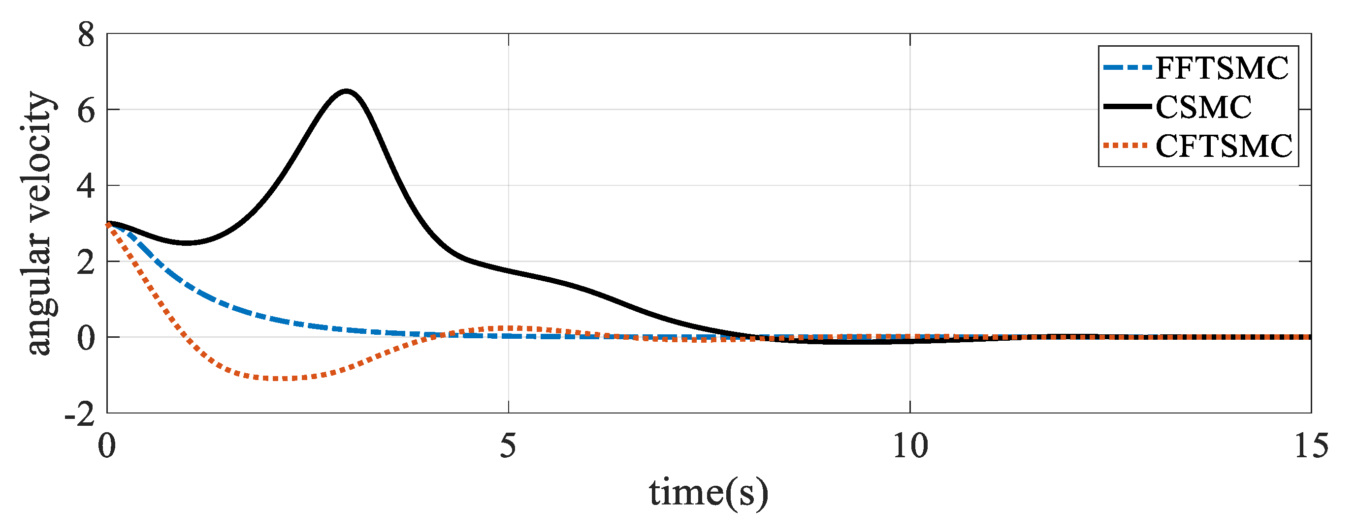
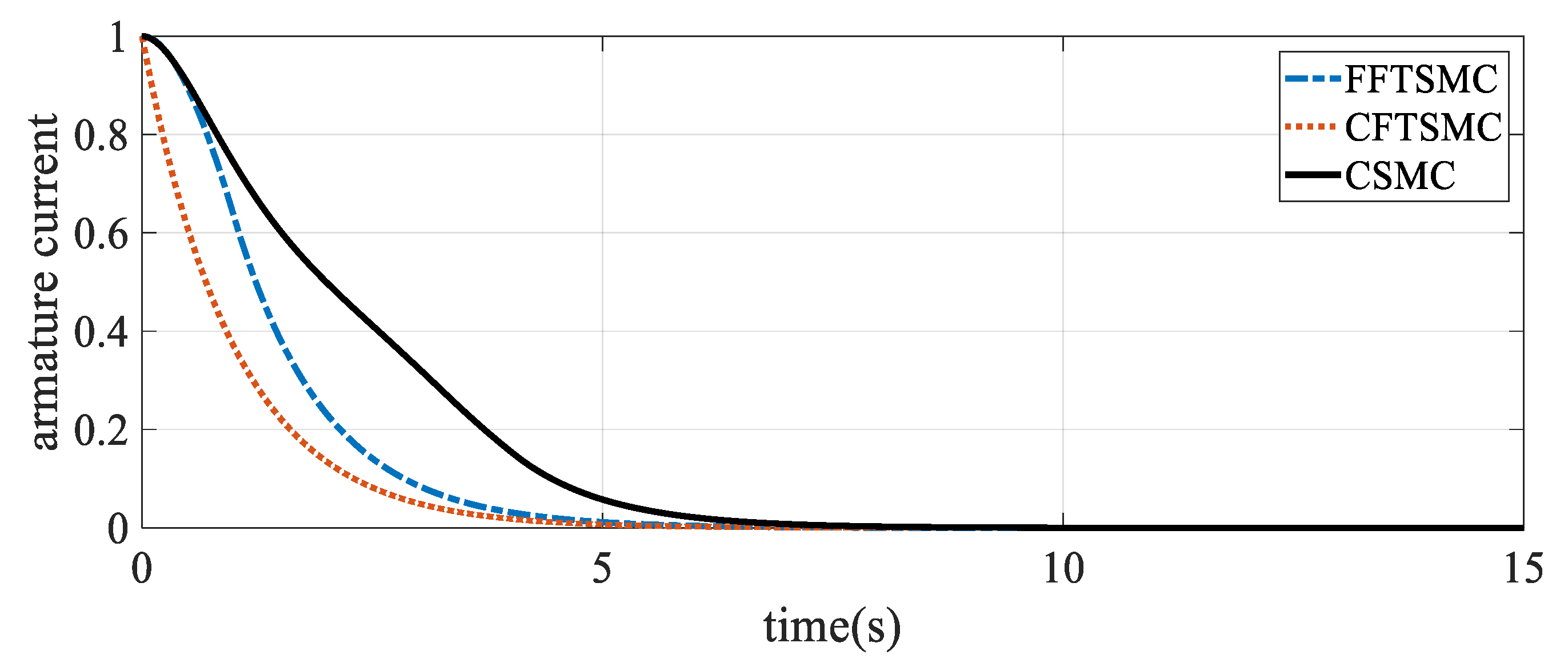
5. Simulation Results

Consider a DC servo motor represented by [38]:

$$\begin{gathered} {\dot{x}}_1\left(t\right)=\left[\begin{array}{cc}0& 1\\ 0& -0.694\end{array}\right]x_1\left(t\right)+\left[\begin{array}{c}0\\ 112.36\end{array}\right]x_2\left(t\right) \\ {\dot{x}}_2\left(t\right)=\left[\begin{array}{cc}0& -161.8\end{array}\right]x_1\left(t\right)-1500x_2\left(t\right)+200u\left(t\right)+20 \sin \left(10x_2\left(t\right)\right) \\ y\left(t\right)=\left[\begin{array}{ccc}1& 0& 0\end{array}\right]x\left(t\right) \end{gathered}$$

(49)

where $x_1\left(t\right)={\left[\begin{array}{cc}\theta & \dot{\theta }\end{array}\right]}^T$ represents the angular velocity and the angular position. $x_2\left(t\right)=i$ is the armature current. The parameters of the servomotor considered in this simulation study are provided in

Table 2. Parameters of the DC servo motor.

Parameters	Values
Armature Resistance (R)	$7.5 \mathsf{\Omega }$
Armature Inductance (L)	$5 \mathrm{mH}$
Motor inertia (J)	$0.006{ \mathrm{kgm}}^2$
Friction Constant (B)	$0.005 \mathrm{Nms}$
Torque constant$\mathit{\left(}{\mathit{K}}_{\mathit{t}}\mathit{\right)}$	$0.809 \raisebox{1ex}{$\mathrm{Nm}$}\!\left/ \!\raisebox{-1ex}{$\mathrm{A}$}\right.$
Back emf constant$\mathit{\left(}{\mathit{K}}_{\mathit{e}}\mathit{\right)}$	$0.809 \raisebox{1ex}{$\mathrm{Vs}$}\!\left/ \!\raisebox{-1ex}{$\mathrm{rad}$}\right.$
Rated Speed	$1500 \raisebox{1ex}{$\mathrm{r}$}\!\left/ \!\raisebox{-1ex}{$\min $}\right.$

[30]. The desired values are defined as $x_d={\left[\begin{array}{ccc}0& 0& 0\end{array}\right]}^T$. The initial values are set as: $x\left(0\right)=\left[\begin{array}{ccc}\frac{\pi }{3}& 3& 1\end{array}\right]$. $\raisebox{1ex}{$p$}\!\left/ \!\raisebox{-1ex}{$q$}\right.$ is selected equal to 7/9. $P=\left[\begin{array}{cc}99.565& 0.001\\ 0.001& 0.004\end{array}\right], W=\left[\begin{array}{cc}7.918& 0.151\\ 0.151& 24.841\end{array}\right]$ and $Q=\left[\begin{array}{cc}\mathrm{18,141.89}& 0\\ 0& \mathrm{18,141.89}\end{array}\right]$. These are the obtained values by using the LMI MATLAB toolbox. The parameters ${\mu }_1$ and ${\mu }_2$ are found as ${\mu }_1=99.565$ and ${\mu }_2=24.867$. Figure 1 shows the membership function of $e,$ which is based on Table 1.

Figure 2 shows the membership function of $\dot{e},$ which is designed based on Table 1. By choosing smaller intervals for $e$ and $\dot{e}$, the overshoot and error are decreased and the error signal converges to zero more quickly.

The proposed approach is compared to the classic fast terminal sliding mode control (CFTSMC) method [39] and classic sliding mode control (CSMC) [21,40], which considers the control of spacecraft electromagnetic docking and DC servo motor. The dynamics of the sliding surfaces for all three approaches are depicted in Figure 3.

As shown in Figure 3, the chattering related to the sliding surface and overshoot are reduced by using fuzzy. The control signal is shown in Figure 4. The control signals for all three approaches are shown in Figure 4. Note that the (FFTSM) control signal is simpler and has less oscillations.

Figure 5 shows the convergence of the angular position to the desired value. The angular position starts with the $\frac{\pi }{3}$ initial value and converges to zero.

Table 3. Comparison between three control methods for angular position.

Controller	Time of Convergences to Zero Tracking Error	Control Signal Range	Chattering Phenomenon	$\mathit{ISV}\left(\mathit{u}\right)$	IAE
Proposed method	$7.315 \left(\mathrm{s}\right)$	$-2.2932$$\mathrm{to} 0.1101$	No	$1.2942$	$1.1635$
CFTSM	$7.510\left(\mathrm{s}\right)$	$-2.2932 \mathrm{to} 0.2157$	No	$1.9397$	$1.2605$
CSM	$\infty$	$-1\mathrm{e}-3 \mathrm{to} 0.5201$	Yes	$2.6511$	$88.8725$

examines the comparison between the three control methods for the angular position. Note from Table 3 that the advantages of the proposed method are the fast and finite-time convergence to the reference trajectory and robustness to parametric uncertainties and external disturbances. The error signal is converged to zero and the ISV and IAE criteria [41] are smaller than the other methods. Moreover, unlike the CSMC approach, the proposed method is free of the chattering phenomenon.

Note that we can infer from Table 3 that the proposed approach yields a control signal with smaller amplitude that of the two other approaches. Note also that the proposed approach yields chattering-free dynamics. Figure 6 shows the dynamics of the angular velocity.

Note from the above figure that tracking to the desired value occurs faster with the proposed controller. Figure 7 shows the convergence of the armature current to the desired value.

Note that the proposed approach results in armature current that tracks its reference value much faster than the other approaches and without any chattering. All the obtained results confirm the superior performance of the proposed approach in terms of faster finite-time convergence of the system states to the equilibrium and chattering-free dynamics.

6. Conclusions

This paper proposed an LMI-based fuzzy fast terminal sliding mode control technique for MIMO uncertain systems. The fast terminal sliding mode control scheme is used to reach the desired value more quickly. The control parameters are obtained using the LMI approach. Fuzzy logic is considered to adjust the sliding surface and switching control gains and further improve the system’s dynamic response. The performance of the proposed approach was assessed using a DC motor. The obtained results showed that the proposed approach yields control gains with smaller ranges, ensured fast finite-time convergence of the system states to their references, and resulted in chattering-free dynamics.

References

1. Chen, R.; Wang, Z.; Che, W. Adaptive Sliding Mode Attitude-Tracking Control of Spacecraft with Prescribed Time Performance. Mathematics 2022, 10, 401. [Google Scholar] [CrossRef]
2. Khalil, H.K. Nonlinear Systems, 3rd ed.; Patience Hall: Hoboken, NJ, USA, 2002; p. 115. [Google Scholar]
3. Spurgeon, S. Sliding Mode Control: Theory and Applications; CRC Press: Boca Raton, FL, USA, 1998. [Google Scholar]
4. Mobayen, S. An LMI-based robust controller design using global nonlinear sliding surfaces and application to chaotic systems. Nonlinear Dyn. 2015, 79, 1075–1084. [Google Scholar] [CrossRef]
5. Mobayen, S. Design of LMI-based sliding mode controller with an exponential policy for a class of underactuated systems. Complexity 2016, 21, 117–124. [Google Scholar] [CrossRef]
6. Levant, A. Homogeneity approach to high-order sliding mode design. Automatica 2005, 41, 823–830. [Google Scholar] [CrossRef]
7. Wu, Y.; Yu, X.; Man, Z. Terminal sliding mode control design for uncertain dynamic systems. Syst. Control Lett. 1998, 34, 281–287. [Google Scholar] [CrossRef]
8. Zhihong, M.; Yu, X.H. Terminal sliding mode control of MIMO linear systems. IEEE Trans. Circuits Syst. I: Fundam. Theory Appl. 1997, 44, 1065–1070. [Google Scholar] [CrossRef]
9. Liu, J.; Sun, F. A novel dynamic terminal sliding mode control of uncertain nonlinear systems. J. Control Theory Appl. 2007, 5, 189–193. [Google Scholar] [CrossRef]
10. Behnamgol, V.; Vali, A.R. Terminal sliding mode control for nonlinear systems with both matched and unmatched uncertainties. Iran. J. Electr. Electron. Eng. 2015, 11, 109–117. [Google Scholar]
11. Yu, X.; Zhihong, M. Fast terminal sliding-mode control design for nonlinear dynamical systems. IEEE Trans. Circuits Syst. I: Fundam. Theory Appl. 2002, 49, 261–264. [Google Scholar]
12. Yang, L.; Yang, J. Nonsingular fast terminal sliding-mode control for nonlinear dynamical systems. Int. J. Robust Nonlinear Control 2011, 21, 1865–1879. [Google Scholar] [CrossRef]
13. Yang, L.; Yang, J. Robust finite-time convergence of chaotic systems via adaptive terminal sliding mode scheme. Commun. Nonlinear Sci. Numer. Simul. 2011, 16, 2405–2413. [Google Scholar] [CrossRef]
14. Mobayen, S. Fast terminal sliding mode tracking of non-holonomic systems with exponential decay rate. IET Control Theory Appl. 2015, 9, 1294–1301. [Google Scholar] [CrossRef]
15. Xu, S.S.-D.; Chen, C.-C.; Wu, Z.-L. Study of nonsingular fast terminal sliding-mode fault-tolerant control. IEEE Trans. Ind. Electron. 2015, 62, 3906–3913. [Google Scholar] [CrossRef]
16. Truong, T.N.; Vo, A.T.; Kang, H.-J. A backstepping global fast terminal sliding mode control for trajectory tracking control of industrial robotic manipulators. IEEE Access 2021, 9, 31921–31931. [Google Scholar] [CrossRef]
17. Mobayen, S.; Baleanu, D.; Tchier, F. Second-order fast terminal sliding mode control design based on LMI for a class of non-linear uncertain systems and its application to chaotic systems. J. Vib. Control 2017, 23, 2912–2925. [Google Scholar] [CrossRef]
18. Wang, H.; Han, Z.-Z.; Xie, Q.-Y.; Zhang, W. Finite-time chaos control via nonsingular terminal sliding mode control. Commun. Nonlinear Sci. Numer. Simul. 2009, 14, 2728–2733. [Google Scholar] [CrossRef]
19. Mobayen, S.; Majd, V.J.; Sojoodi, M. An LMI-based composite nonlinear feedback terminal sliding-mode controller design for disturbed MIMO systems. Math. Comput. Simul. 2012, 85, 1–10. [Google Scholar] [CrossRef]
20. Singh, S.; Janardhanan, S. Fast terminal sliding mode control for twin rotor multi-input multi-output system. In Proceedings of the 2015 Annual IEEE India Conference (INDICON), New Delhi, India, 17–20 December 2015; pp. 1–5. [Google Scholar]
21. Shi, K.; Liu, C.; Sun, Z.; Yue, X. Coupled orbit-attitude dynamics and trajectory tracking control for spacecraft electromagnetic docking. Appl. Math. Model. 2022, 101, 553–572. [Google Scholar] [CrossRef]
22. Qiu, Z.-C.; Zhang, S.-M. Fuzzy fast terminal sliding mode vibration control of a two-connected flexible plate using laser sensors. J. Sound Vib. 2016, 380, 51–77. [Google Scholar] [CrossRef]
23. Song, J.; Zheng, W.X.; Niu, Y. Self-Triggered Sliding Mode Control for Networked PMSM Speed Regulation System: A PSO-Optimized Super-Twisting Algorithm. IEEE Trans. Ind. Electron. 2021, 69, 763–773. [Google Scholar] [CrossRef]
24. Yao, Q. Adaptive finite-time sliding mode control design for finite-time fault-tolerant trajectory tracking of marine vehicles with input saturation. J. Frankl. Inst. 2020, 357, 13593–13619. [Google Scholar] [CrossRef]
25. Nekoukar, V.; Erfanian, A. Adaptive fuzzy terminal sliding mode control for a class of MIMO uncertain nonlinear systems. Fuzzy Sets Syst. 2011, 179, 34–49. [Google Scholar] [CrossRef]
26. Li, T.-H.S.; Huang, Y.-C. MIMO adaptive fuzzy terminal sliding-mode controller for robotic manipulators. Inf. Sci. 2010, 180, 4641–4660. [Google Scholar] [CrossRef]
27. Abrazeh, S.; Parvaresh, A.; Mohseni, S.-R.; Zeitouni, M.J.; Gheisarnejad, M.; Khooban, M.H. Nonsingular Terminal Sliding Mode Control with Ultra-Local Model and Single Input Interval Type-2 Fuzzy Logic Control for Pitch Control of Wind Turbines. IEEE/CAA J. Autom. Sin. 2021, 8, 690–700. [Google Scholar] [CrossRef]
28. Abadi, A.S.S.; Hosseinabadi, P.A.; Mekhilef, S. Fuzzy adaptive fixed-time sliding mode control with state observer for a class of high-order mismatched uncertain systems. Int. J. Control Autom. Syst. 2020, 18, 2492–2508. [Google Scholar] [CrossRef]
29. Yang, Y.; Niu, Y.; Zhang, Z. Dynamic event-triggered sliding mode control for interval Type-2 fuzzy systems with fading channels. ISA Trans. 2021, 110, 53–62. [Google Scholar] [CrossRef]
30. Yang, Y.; Niu, Y.; Reza Karimi, H. Dynamic learning control design for interval type-2 fuzzy singularly perturbed systems: A component-based event-triggering protocol. Int. J. Robust Nonlinear Control 2022, 32, 2518–2535. [Google Scholar] [CrossRef]
31. Feng, Y.; Zhou, M.; Zheng, X.; Han, F.; Yu, X. Full-order terminal sliding-mode control of MIMO systems with unmatched uncertainties. J. Frankl. Inst. 2018, 355, 653–674. [Google Scholar] [CrossRef]
32. Mobayen, S. Design of LMI-based global sliding mode controller for uncertain nonlinear systems with application to Genesio’s chaotic system. Complexity 2015, 21, 94–98. [Google Scholar] [CrossRef]
33. Sun, C.; Gong, G.; Yang, H.; Wang, F. Fuzzy sliding mode control for synchronization of multiple induction motors drive. Trans. Inst. Meas. Control 2019, 41, 3223–3234. [Google Scholar] [CrossRef]
34. Wu, G.; Zhang, X.; Zhu, L.; Lin, Z.; Liu, J. Fuzzy sliding mode variable structure control of a high-speed parallel PnP robot. Mech. Mach. Theory 2021, 162, 104349. [Google Scholar] [CrossRef]
35. Liu, J.; Sun, F. Fuzzy global sliding mode control for a servo system with lugre friction model. In Proceedings of the 2006 6th World Congress on Intelligent Control and Automation, Dalian, China, 21–23 June 2006; pp. 1933–1936. [Google Scholar]
36. Wang, J.; Rad, A.B.; Chan, P. Indirect adaptive fuzzy sliding mode control: Part I: Fuzzy switching. Fuzzy Sets Syst. 2001, 122, 21–30. [Google Scholar] [CrossRef]
37. Zadeh, L. Fuzzy Algorithms. Inf. Control 1968, 12, 94–102. [Google Scholar] [CrossRef] [Green Version]
38. Umeno, T.; Hori, Y. Robust speed control of DC servomotors using modern two degrees-of-freedom controller design. IEEE Trans. Ind. Electron. 1991, 38, 363–368. [Google Scholar] [CrossRef]
39. Yazici, İ.; Yaylaci, E.K. Fast and robust voltage control of DC–DC boost converter by using fast terminal sliding mode controller. IET Power Electron. 2016, 9, 120–125. [Google Scholar] [CrossRef]
40. Qureshi, M.S.; Swarnkar, P.; Gupta, S. Assessment of DC servo motor with sliding mode control approach. In Proceedings of the 2016 IEEE First International Conference on Control, Measurement and Instrumentation (CMI), Kolkata, India, 8–10 January 2016; pp. 351–355. [Google Scholar]
41. Ünsal, S.; Aliskan, I. Investigation of performance of fuzzy logic controllers optimized with the hybrid genetic-gravitational search algorithm for PMSM speed control. Automatika 2022, 63, 313–327. [Google Scholar] [CrossRef]
Figure 1. Membership graph of e .
Mathematics 10 01236 g001
Figure 2. Membership graph of e ˙ .
Mathematics 10 01236 g002
Figure 3. Sliding surfaces for CFTSMC, FFTSMC and CSMC.
Mathematics 10 01236 g003
Figure 4. Comparison between the FFTSMC, CFTSMC and CSMC control signals.
Mathematics 10 01236 g004
Figure 5. Angular position tracking.
Mathematics 10 01236 g005
Figure 6. Angular velocity tracking.
Mathematics 10 01236 g006
Figure 7. Armature current tracking.
Mathematics 10 01236 g007