Comparison of HP Filter and the Hamilton’s Regression

Abstract

In this paper we examine if the use of Hamilton’s regression filter significantly modifies the cyclical components concerning unemployment in Greece compared with those using the Hodrick–Prescott double filter (HP). Hamilton suggested the use of a regression filter in order to overcome some of the drawbacks of the HP filter, which contains the presence of false cycles, the bias in the end of the sample, and the ad-hoc assumptions for the parameters’ smoothing. Thus, our paper examines two widely used detrending methods for the extraction of cyclical components, including techniques of deterministic detrending as well as stochastic detrending. Using quarterly data for the unemployment of Greece in a macroeconomic model decomposition, we indicate that trend components and cycle components of Hamilton’s filter regression led to significantly larger cycle volatilities than those from the HP filter. The dynamic forecasting in the sample, occurred both with autoregressive forecasting, that yields steady forecasts for a wide variety of non-stationary procedures, and with the HP filter, along with its constraints at the end of the time series. The results of the paper showed that the dynamic forecasting of the HP filter is better than that of Hamilton’s in all assessment measures.

1. Introduction

Most economic time series show a behavior that is repeated over the course of time. This allows the modeling of these procedures using techniques that examine the build-up of this procedure on a time period. The application of this methodology consists of ARIMA models as well as state space models. During the processing of time series, we assume that a discrete time series can be analyzed for non-observable components. The non-observable components are long-run trend, seasonal component, cyclical component and the random component. The long-run trend incorporates low frequency volatility, contrary to the cyclical component which incorporates high frequency volatility. Thus, with decomposition we want to extract the cyclical component of the time series which is regarded as the part with the highest periodical variance (volatility) in relation to trend [1]. In order to determine the cyclical component, we should be familiar with business cycles’ behavior, which is a series of macroeconomic studies. One could decomposite the time series with the trend and cyclical component, where trend is used to reflect the long-run development of the series, whereas the cyclical component is the deviation of this series from this trend. In this way, the business cycles, according to [2], are the variances (volatilities) of a time series around a smooth trend. The variances are known as “economic development cycles”.

The decomposition of the time series is motivated by the idea that discrete forces account for long-running growth and variance (volatility) on a time frame which is related with business cycles and seasons. Although the latter is constrained from “seasonal adjustment”, the issue concerning the separation of the trend from the cycle of economic time series such as GDP, unemployment, etc., has been widely discussed for many decades. Various patterns follow alternative approaches and some of them attribute the variance to the cycle trend following a smooth line, and others attribute changes to the level of permanent shocks on the trend.

Moreover, most of economic time series are fluctuating and increasing, thus making the establishment of these types of decomposition extremely difficult, especially when we try to perform this decomposition on data in an emerging economy. A significant issue that occupies decomposition methods is the nature of trend. It is necessary to recognize the differences between trend, stationarity, and stochastic trend. Trend is regarded as a linear, deterministic trend that is affected by external transitory changes. On the other hand, stochastic trend is referred to as a random walk with a significant quantity of noise. It is important to examine whether we have permanent effects on the trend, similarly to the cyclical components, where we can assume that they also present stochastic phenomena.

In many studies related to business cycles, researchers avoid dealing with the trend forms, instead adopting a generally accepted recipe for trend. In our paper, we adopt two of the most widely applied decomposition methods of series components such as [3] filter and [1] which can recognize trend components, cycle components, and noise that are in different frequencies. Applying these techniques, one can decompose a time series with a number of sine and cosine functions that determine the rate at which the time series is oscillating.

The arguments concerning the advantages and disadvantages of the use of empirical modeling on both filters in the literature vary [4,5,6,7,8,9]. Some papers point out that the HP filter causes spurious cycles when it is applied to statistical data. Others claim that the HP filter is better approached with a random walk, and thus a difference stationary process. However, when Hamliton’s filter is applied on a random walk, it is transformed in a difference filter, so some cyclical frequencies are reformed or cancelled.

It is suggested that Hamilton’s filter is applied to differences of stationary data, whereas the HP filter does not use these differences. In this paper, using a macroeconomic decomposition model for unemployment in Greece, a comprehensive framework is provided both for analysts and users. We assume that the HP filter gives a useful trend on the series. Moreover, trend variations when using the HP filter are regarded as providing reliable estimations on business cycles of the series in relation to those of Hamilton’s filter, particularly during critical economic periods on dates where unemployment increases. Moreover, the comparison between these two filters has not been done. This paper tries to deal with the gap using unemployment in Greece. Moreover, in this paper we compare the quality of expansion on forecasting, using trend estimations for forecasting on the ex post forecasting of the HP filter on series end points.

The structure of the paper is as follows. In Section 2, the methodological framework is presented, which consists of the decomposition of series, the exponential smoothing filter, the Hodrick and Prescott (HP) filter, and the Hamilton (HF) regression filter. The critiques from various researchers for both filters are provided in Section 3. Section 4 presents and analyses the data. The results on the estimation of the filters are given in Section 5. Forecasting procedures and the results of the two filters are analyzed in Section 6. Finally, in Section 7 conclusions are given.

2. Methodological Framework

The decomposition of macroeconomic time series in trends and cyclical components are of vital importance for many macroeconomic definitions such as gross domestic product, interest rate, unemployment, and so on. This means that short and long-run movements can be differentiated. Typically, the components are theoretical definitions, and thus, they are non-observable. Let us assume that time series $y_t$ accepts the additive decomposition which can be expressed as:

$$y_t=g_t+c_t$$

(1)

where $g_t$ is a hidden or non-observable trend and $c_t$ is the deviation from the trend.

The decomposition and its semantic components are defined, assuming that $g_t$ is smooth and follows the general movement of the time series, whereas $c_t$ reflects the short-run variances and cyclical behavior which is not taken into account from the trend. Ultimately, $g_t$ is the basic average level around which the deviations of cyclical components are estimated in the short-run, just like business cycles. The $g_t$ is estimated from the following linear trend filter: (see [8]).

$${\widehat{g}}_t={\displaystyle \sum _s{w}_t(s)y_{t-s}}$$

(2)

with the deviations of the trend to be calculated from the following type:

$${\widehat{c}}_t=y_t-{\widehat{g}}_t={\displaystyle \sum _s{\widehat{w}}_t(s)y_{t-s}}$$

(3)

where ${\widehat{w}}_t(s)=-w_t(s)$ for $s\ne 0$ and ${\widehat{w}}_t(0)=1-w_t(0)$.

The weights of filter $w_t(s)$ can be a time-varying or time-invariant where $w_t(s)=w(s)$. Many filters used in the analysis of business cycles can be used in a general form, such as the Hodrick–Prescott filter where $w_t(s)$ varies in terms of temporality (see [8]). In the literature, many tools have been developed for trend extraction. Reviews related to trend cycle decomposition are given from [10,11,12].

2.1. The Exponential Smooth Filter

The meaning of time series smoothing is referred to as the decrease or eradication of variance from this series. The exponential smoothing was suggested at the end of 1950 from [13,14,15], and is regarded as one of the most successful forecasting methods. Forecasts deriving from the use of exponential smoothing methods are weighted averages of previous data, and weights decompose exponentially as the sample grows. Exponential smoothing covers a wide range of methods, including some recent ones, such as long-run approaches of undivided exponential smoothing and linear methods of Holt, that still hold central places in this sector analysis. The choice of method is based on the recognition of basic time series components (trend and seasonality) and the way that they insert themselves in the smoothing method (for example in an additive, damped or multiplicative way). Smoothing methods have been used by [16] in the framework of permanent income analysis and from [2] in various empirical studies.

According to [17], the exponential smoothing is based on the likelihood of errors-trends-seasonality and can be considered as a two-sided filter that can attribute stationary series which are characterized from stochastic trends. The exponential filter is a low pass filter which is destined to pass through flow frequencies, reducing high frequencies. It has only one tuning parameter (apart from the sample interval) and requires saving only one variable.

The exponential filter is an autoregressive filter, and its use is characterized as “exponential smoothing”. In various sectors, such as investment analysis, the exponential filter is called “exponentially weighted moving average term” or simply “exponential moving average”. This term abuses the traditional terminology ARMA “moving average” of time series analysis because we do not use prior values, only current values.

Thus, the filter of exponential smoothing offers the permanent component of series $y_t$ as a solution to the following minimization problem:

$$\min \left\{g_t\right\}{\displaystyle \sum _{t=1}^T\left[{\left(y_t-g_t\right)}^2+\lambda {\left(g_t-g_{t-1}\right)}^2\right]}$$

(4)

Parameter $\lambda$ penalizes the changes on the permanent component $g_t$ of series $y_t$. The smoothing rank of the estimated component $g_t$ depends on the selected value of parameter $\lambda$. The first order condition for minimizing the above function takes the following form:

$$-2(y_t-g_t)+2\lambda (g_t-g_{t-1})-2\lambda (g_{t+1}-g_t)=0$$

(5)

The above condition shows the relationship between transitory component $c_t=y_t-g_t$ and the changes of permanent component $g_t$.

2.2. The Creation of the Hodrick and Prescott Filter

The [3] filter is the best known and is a widely univariate method for the decomposition of time series. They are used by International Organizations such as the International Monetary Fund (IMF), and also by Central banks such as the European Central Bank. It is a smoothing method used in macroeconomics, especially on theories of real business cycles, in order to extract the cyclical component of the time series from raw data. The adjustment of a trend in short-run variances is accomplished with the modification of the multiplier $\lambda$. The Hodrick–Prescott (HP) filter decomposes from a time series $y_t$, the trend component $g_t$, and cyclical component $c_t$, $y_t=g_t+c_t$.

The estimation of the decomposition of a trend component is taken through the minimization of the following function:

$$\min \left\{g_t\right\}{\displaystyle \sum _{t=1}^T\left\{{\left(y_t-g_t\right)}^2+\lambda {\left[\left(g_{t+1}-g_t\right)-\left(g_t-g_{t-1}\right)\right]}^2\right\}}$$

(6)

The cyclical component is found by extracting a trend component from the time series. $c_t=y_t-g_t$.

From the above function we can see that the minimization of component $g_t$ is given from the sum of squares of the variance of the time series from component $g_t$ (the first term of the function), and from the sum of squares of the transitive component, which is penalized for the change to the second difference of component $g_t$ (second term of function). Parameter $\lambda$ is related to trend smoothing. Thus, the above function can be re-written as follows:

$$\min \left\{g_t\right\}{\displaystyle \sum _{t=1}^T\left\{d^2+\lambda {\left[{\mathrm{\Delta }}^2{g}_{t+1}\right]}^2\right\}}$$

(7)

The above function can be expressed as a system of linear equations of time series $y_t$, as a function of $g_t$, and via a matrix of A dimensions $T\times T$

$$y_t=A{g}_t$$

(8)

where $y_t$ and $g_t$ are column vectors $T\times 1$.

The first order for the minimization of the function is written as follows:

$$c_1=y_1-g_1=\lambda (g_1-2g_2+g_3)$$

$$c_2=y_2-g_2=\lambda (-2g_1+5g_{2}4g_3+g_4)$$

$$c_t=y_t-g_t=\lambda (g_{t-2}-4g_{t-1}+6g_t-4g_{t+1}+g_{t+2})$$

$$c_{T-1}=y_{T-1}-g_{T-1}=\lambda (g_{T-3}-4g_{T-2}+5g_{T-1}-2g_T)$$

$$c_T=y_T-g_T=\lambda (g_{T-2}-2g_{T-1}+g_T)$$

The following equations in a matrix are provided below:

$$y_t-g_t=\lambda Fg$$

(9)

where:

$$\underset{(T\times T)}{\underbrace{F}}=\left[\begin{array}{cccccc}1& -2& 1& 0& 0& \mathrm{0...0}\\ -2& 5& -4& 1& 0& \mathrm{0...0}\\ 1& -4& 6& -4& 1& \mathrm{0...0}\\ 0& 1& -4& 6& -4& 1\dots 0\\ \dots & \dots & \dots & \dots & \dots & \dots \dots \\ 0& 0& 0& 0& 0& \mathrm{0...1}\end{array}\right]$$

The permanent component $g_t$ in a matrix form is as follows:

$$g_t=A^{-1}{y}_t={\left(\lambda F+I\right)}^{-1}{y}_t$$

(10)

King and Rebelo [18] studied the circumstances where the Hodrick and Prescott filter works as the best filter. These circumstances are special and sometimes contradict the economic theory of business cycles. Finally, Harvey and Jaeger [19] studied the circumstances under which the HP filter minimizes the mean square error.

$$MSE=\frac{1}{T}{\displaystyle \sum _{t=1}^T{({\widehat{d}}_t-d_t)}^2}$$

(11)

where $d_t$ is a real cyclical component and ${\widehat{d}}_t$ is the estimated component. Let us assume that both the trend component and cyclical component follow ARMA processes where their innovations are not correlated, thus we get:

$$A^g(L)g_t=M^g(L)e_t^g$$

(12)

$$A^d(L)d_t=M^d(L)e_t^d$$

(13)

where $e_t^g$ and $e_t^d$ are serially and independently errors with variances, ${\sigma }_g^2$ and ${\sigma }_d^2$. AR polynomial $A^g(L)$ for the trend component can contain more than one unit root.

Whittle [20] shows the optimal filter for cyclical component $d_t$ and is provided below:

$$H_d(L)=\frac{\psi A^g(L)A^g(L^{-1})}{\psi A^g(L)A^g(L^{-1})+(1-\psi )Q(L)}$$

(14)

where

$$\psi =\frac{{\sigma }_d^2}{{\sigma }_d^2+{\sigma }_g^2}$$

and

$$Q(L)=\frac{A^d(L)A^d(L^{-1})M^g(L)M^g(L^{-1})}{M^d(L)M^d(L^{-1})}$$

In comparison with other filters, the estimated trend for the Hodrick–Prescott filter is more sensitive to temporal shocks or short-run variances at the end of the sample. This results in a suboptimal return for the Hodrick–Prescott filter in the final places of the time series [21].

The Value of $\lambda$

Matrix A depends on the number and the frequency of observations, and it also depends on parameter $\lambda$. Thus, it is understandable that the role of parameter $\lambda$ on the filter is vital. Given that parameter $\lambda$ has the basic properties of the HP filter, many critiques have been levelled at its proper value; however, there is no clear evidence about the choice of the suitable value of $\lambda$. The choice of the value of $\lambda$ should be adjusted so that we can be aware of the cycle’s duration. The smoothing parameter $\lambda$ does not affect the cycle or the instability of the trend’s increase, a fact that proves that the HP filter does not contain a model for the cycle.

With lower values for the smoothing parameter $\lambda$, the trend becomes more volatile, for it contains a larger part of the spectral of high frequencies. If $\lambda =0$, Function (6) is minimizing with $y_t=g_t$, meaning that the permanent component (trend component) is identified with the time series and there is no cyclical component. Increasing the value of $\lambda$, we obtain more smooth estimations of the trend component $g_t$, and more unstable estimations of the cyclical component $c_t$. For $\lambda \to \infty$, Function (6) is minimized, and the estimated trend converges on the linear trend of the least squares, thus becoming a straight line. Moreover, in the case where $\lambda =0$, the trend becomes equal with the earliest series, so a cyclical component does not exist.

The suggested values for $\lambda$ are given from $\lambda =100\times N^2$, where $N$ is the frequency of series $y_t$ ($N=1,4,12$ for annual, quarterly, and monthly data, respectively). For quarterly data, Hodrick and Prescott claim that $\lambda =1600$. Nevertheless, there is an agreement related to the value used when the filter is applied to other frequencies (annual and monthly). For annual data, many researchers such as [22] used the value $\lambda =100$ assuming that the cyclical component is 10 times more volatile from the change of the time series. Ravn and Uhlig [23] suggest that $\lambda$ should differ to the power of four of the observed frequency ratio; therefore, $\lambda$ must be equal with 6.25 $\left(\frac{1600}{4^4}\right)$ for annual data and 129,600 $\left(1600\times 3^4\right)$ for monthly data.

Thus, many researchers choose high values for $\lambda$ when filtering annual data because they claim that low values provoke unstable growth rates. Kaiser and Maravall [24] suggest the value 8 for annual data and [25] supports the value $\lambda =1000$ for quarterly data, and $\lambda =$ 3 to 5 for annual data. Bouthevillain et al. [26] show that the filter is applied with $\lambda =30$ and [27] with $\lambda =20$ on annual data.

2.3. The Hamilton (2018) Filter

Some points of the Hodrick–Prescott (HP) filter have been criticized by a paper [1] entitled “Why you should never use the Hodrick–Prescott filter”, which has drawn the attention of researchers. Hamilton criticized the Hodrick–Prescott (HP) filter due to three drawbacks:

• The HP filter produces series with spurious dynamic relationships (spurious cycles).
• The filtered values at the end of the sample are much different from those which are in the sample mean.
• The statistics of the standard problem produce high values for the smoothing parameter $\lambda$ compared with common practice.

Hamilton offers an alternative, easy-to-handle recipe that avoids the weaknesses of the Hodrick–Prescott procedure. He suggests a regression filter, as an alternative solution to the disadvantages of HP filter, using forecasts of the series to remove the cyclical nature. Hamilton [1] suggests an alternative procedure that avoids the framework of the model $y_t=g_t+c_t$, with the unobservable trend $g_t$, and the trend deviation $c_t$. He claims that the information of business cycles can be gathered immediately from the estimations of time series $y_t$ with an OLS method using suitably selected error forecasts. More specifically, Hamilton uses a forecasting model of autoregression and develops the decomposition of a non-stationary time series on trends and cyclical components with the estimation of the following regression $y_{t+h}$ on a constant, using a current value of $y_t$, and on $p-1$ series lags.

$$y_{t+h}={\beta }_0+{\beta }_1{y}_t+{\beta }_2{y}_{t-1}+{\beta }_3{y}_{t-2}+{\beta }_4{y}_{t-3}+e_{t+h}$$

(15)

where:

$y_{t+h}$ is the value of series $y_t$ for h periods ahead.

Trend component of time $t+h$ is given from the following regression:

$$g_{t+h}={\widehat{\beta }}_0+{\widehat{\beta }}_1{y}_t+{\widehat{\beta }}_2{y}_{t-1}+{\widehat{\beta }}_3{y}_{t-2}+{\widehat{\beta }}_4{y}_{t-3}$$

(16)

The cyclical component on time $t+h$ is defined as the deviation of value $y_{t+h}$ from the estimation of the trend component $g_{t+h}$. Thus, we get:

$$c_{t+h}=y_{t+h}-g_{t+h}$$

(17)

According to Equations (15)–(17), the cyclical component is created from the residuals of Equation (15)

$$c_{t+h}=e_{t+h}=y_{t+h}-{\widehat{\beta }}_0-{\widehat{\beta }}_1{y}_t-{\widehat{\beta }}_2{y}_{t-1}-{\widehat{\beta }}_3{y}_{t-2}-{\widehat{\beta }}_4{y}_{t-3}$$

(18)

Furthermore, Equation (18) is based on the results of [28], which presents that error forecasting is stationary for a wide range of non-stationary procedures. Moreover, Hamilton’s filter has the advantage of there being no need to know the procedure for the creation of the data before applying them. In addition, according to [1], the filter’s regression reduces a difference on the filter, when applied to a random walk. In other words, if $\mathrm{\Delta }{y}_t$ is a stationary series, the sum of the coefficients’ slope for Equation (15) will converge on large samples, thus Equation (15) will be equal to the following regression:

$$y_{t+h}-y_t={\delta }_0+{\delta }_1\mathrm{\Delta }{y}_t+{\delta }_2\mathrm{\Delta }{y}_{t-1}+{\delta }_3\mathrm{\Delta }{y}_{t-2}+e_{t+h}$$

(19)

Hamilton [1] indicates that if forecasting is low, the left side of Equation (19) will indicate that cyclical fluctuations are similar to those found in the 8th data difference. In such a circumstance, the cyclical component will be denoted as:

$$c_{t+h}=y_{t+h}-y_t$$

(20)

Moreover, error forecasting is the difference

$${\widehat{e}}_{t+h}=y_{t+h}-y_t$$

(21)

In the case of quarterly data, [1] suggested the use of h = 8 for analysis concerning business cycles and h = 20 for studies concerning financial or credit cycles, as it was developed by [29] which used annual data for h = 5. Thus, Hamilton uses h = 20, which means that it is 5Χ4. The four lags that Hamilton uses for the observed series, share attributes with the stationary residuals, since the fourth differences on the initial series are stationary.

A number of studies have provided theoretical as well as empirical valuations of Hamilton’s suggested methodology, such as [4,5,6,30,31,32], and also [9].

3. Critique of Hodrick–Prescott and Hamilton Filters

Hamilton [1] of his paper entitled “Why you should never use the Hodrick–Prescott filter”, presents data against the use of the Hodrick–Prescott filter, which are the following:

• The Hodrick–Prescott filter produces series with spurious dynamic relationships which do not have a basis in the procedure of data creation.
• The filtered values at the end of the sample are different from those in the middle and are characterized from spurious dynamics.
• The statistics of the standardized problem usually produce large values for smoothing parameter $\lambda$, in comparison with the common practice; for example when the $\lambda$ value is below 1600 for quarterly data.
• Hamilton, in his paper, suggests a better alternative solution. A regression on $t+h$ date on the four closest values from date t offers a strong approach for obtaining all the goals that the users of the Hodrick–Prescott filter are looking for, whilst avoiding the filter’s shortfalls.

Which is the alternative suggested by Hamilton? Hamilton avoids the framework of Model (1) with the non-observable trend $g_t$ and with the deviation of trend $c_t$. On the contrary, he claims that business cycle information can be collected directly from time series $y_t$, using suitably selected forecasting OLS error from an autoregression model.

Afterwards, [31], in his paper entitled “An exploration of trend-cycle decomposition methodologies in simulated data” examines if the suggested alternative prοcedure of Hamilton is better than the Hodrick–Prescott filter on the extraction of a cyclical component from many simulated time series in order to approach the real GDP of the USA. Hodrick ascertains that for the time series where there are discrete developing and cyclical components, the Hodrick–Prescott filter approaches the isolation of the cyclical element against Hamilton’s alternative solution.

A second critique of Hamilton is relevant to the capability of the HP filtered data that causes cycles where they do not exist. When [33] supported the idea that the linear detrending of a time series, which is considered as random walk, causes spurious periodicity as a function of length sample, [34] proved that the application of the HP filter on a series that is a random walk enforces the complex dynamic properties in its development, and in cyclical components that apparently do not exist. As is the case for every two-sided filter, observations at the beginning and end of the sample have different weights for development components; indeed, those that are far away from the end distort the dynamic of the cyclical component. It is worth noting that the critiques are applied to every filter technique. Furthermore, Hodrick realizes that the HP and BK filters are similar, and that Hamilton’s filter operates better when series are stationary on first differences.

We present below, in detail, the drawbacks of the Hodrick–Prescott filter, as Hamilton claims, and we put them under a wider perspective [35].

3.1. Spurious Dynamics

The basic criticism for the HP filter is that it introduces dynamic normalities that are unrelated to the process of data creation. Hamilton [1] added up the asymptotic properties of stochastic procedures on mathematical analysis and used spectral densities and power transfer functions referred to data from random walk procedures. One can accept a random walk on trend, but asymptotic statistics are not necessarily determinant. Nevertheless, such a series does not usually appear, so the HP detrended series can properly forecast.

3.2. End-of-Period Bias

For many time series on the two ends of the sample, the trend line of the HP bends towards actual observations. However, the whole research sample can be cut back by a few quarters. Thus, if the detrending only aims at designated events of business cycles, then bias at the end of the period is not considered an argument against the HP filter. Bias becomes meaningful if the HP filter is used for analysis in real time or in macroeconomic forecasts. On such occasions, researchers should examine this bias. In spite of these issues, the HP filter, if not used as the only reference, can be helpful if it is modified with two small adjustments; a lower value for smoothing parameter $\lambda$ and a rescaling of the extracted cyclical component (see [7]). Finally, Hamilton [1] does not prove anything in his article, and again, his negative judgment is based on a random walk.

3.3. Doubts about the Conventional HP Smoothing Parameter

On trend decomposition and business cycles we assume that these two components do not present a common pattern; however, this does not occur with the HP filter and the conventional smoothing coefficient $\lambda$ = 1600 for quarterly data. At this point we should stress the drawbacks of the HP filter; however, many researchers, although they realize this drawback, they insist that the smoothing parameter should stay the same. In this case, Hamilton claims that the last component for the decomposition of trend-cycle is white noise. Under this assumption, the value of parameter $\lambda$ can be estimated with the maximum likelihood method. In addition, he supports the remedy for the excessive flexibility on the trend line as the highest value for $\lambda$ coefficient. Even if he argues all of these in his paper with 13 macroeconomic variables, the value of the coefficient is lower than $\lambda$ = 1600 and in fact much lower.

Schuler [4] proves that the Hamilton regression filter shares some of the drawbacks of the Hodrick–Prescott filter. For example, Hamilton’s ad hoc statement for a two-year regression filter entails a cancellation of two-year cycles and an augmentation of cycles longer than typical business cycles. This is in contrast with stylized business cycle facts, such as the one-year duration of a typical recession leading to inconsistencies with the chronology of the business cycle, according to the National Bureau of Economic Research Studies (NBER). Nevertheless, Hamilton’s regression filter is preferable to the HP filter in creating a credit-to-GDP gap.

Drehmann and Yetman [30] referred to the credit gap defined by the deviation of the credit-to-GDP ratio from a filtered HP trend and is considered to be a strong indicator of a prompt warning for crisis forecasting. Hamilton [1], however, claims that the HP filter should never be used as it leads to spurious dynamics, presents problems for the last benchmark, and its application is in contrast with its statistical foundations; conversely, he suggests the use of linear projections. Some also criticized GDP smoothing as the gaps will negatively correlate with production. However, with a lack of clear theoretical foundations, all suggested gaps are no more than indicators; hence, a good empirical question measures yields as a warning indicator for crises. Drehmann and Yetman [30] use quarterly data from 1970 until 2017 for forty-two economies and realize that no other gap exceeds the credit-to-GDP gap. Conversely, credit gaps based on linear projections in real time perform poorly.

Jonsson [5] has evaluated the HP and Hamilton filters for spurious dynamics on the cyclical component of a business cycle, and mentioned that spurious dynamics can be found on the cyclical element on both filters. Thus, he could not suggest which filter can be used for trend decomposition and cycle decomposition in a series.

Jonsson [6] compares the HP filter and Hamilton filter in relation to the stability of real time, using the estimation of the GDP gap for the USA, and realizes that the Hamilton filter outweighs the HP filter when it comes to real-time repetitions. This is owed to the fact that trend estimations and cycle estimations of the HP filter at the end of the sample are revised to a large degree as more data are added to the series.

Wolf et al. [7] indicates that a one-sided HP filter should not be used as it fails to extract the low frequency of fluctuations, and dampens fluctuations in all frequencies, even those that intends to extract. Wolf et al. [7] suggest two small adjustments to the one-sided HP filter, thus aligning the properties with that of the two-sided HP filter. This means a lower value for the smoothing parameter and a multiplicative rescaling of the extracted cyclical component.

Quast and Wolters [32] suggest a modification of Hamilton’s filter which yields reliable and economically significant estimations on gap production in real time. Hamilton’s filter is based on error forecasting of eight quarters before a simple autoregression of real GDP. Even though this procedure yields a cyclical component that is hardly reconsidered due to the new incoming data from the one sided filter, it does not cover the typical frequencies of the economic cycle because it deletes the small cycles and also amplifies the medium length cycles. Moreover, as the estimated trend contains high-frequency noise, it can hardly be interpreted as potential GDP. A modification of [32] based on the average of error forecasting from four to twelve quarters ahead, leads to a better coverage of the typical frequencies of an economic cycle and a smooth estimated trend from the initial Hamilton’s filter.

Phillips and Shi [9] develop a boosted HP filter (bHP) and analyze its relative attribution on Hamilton’s regression. Their findings present an explicit preference for the HP filter over Hamilton’s regression and supports the conclusion that the HP filter can be used as an auxiliary empirical device for the estimation of trends and cycles.

Hall and Thomson [8], within a framework of a business cycle for New Zealand, evaluates whether Hamilton’s filter (H84), using OLS estimation, produces stylized facts that differ from the Hodrick –Prescott (HP) and Baxter–King (BK) filters; it also evaluates whether the use of predictive filter H84, which expands forecasting, improves the HP filter at the end of the series. On their paper concerning business cycles, they use a total of basic macroeconomic variables, as well as quarterly, seasonally adjusted data. The results of their paper showed that H84 produces greater volatilities and less credible trend movements during fundamental economic periods from the HP filter so there is no advantage to using H84 through the HP filter.

Some researchers allow the creation of multivariate economic models and the parameters’ adjustment on data, such as models with non-observable components (UC) in addition to clear mechanical mechanisms of raw data such as the Baxter–King filter [21] and Hodrick–Prescott filter [3]. From a theoretical perspective, these complex models with unobservable data are superior to simple methods. From a practical perspective, the estimation of a non-observable component is performed using recursive estimation such as the Kalman filter.

Apart from the aforementioned filters, other filters constructed on the basis of standard local polynomial regression (LPR) methods have been used for the estimation of business cycles. More specifically, [36] used quarterly data for the GDP of the USA from 1947:1−2016:2, and the methods of high-pass local polynomial regressions for the business cycles of GDP for USA with different functions of kernel and bandwidths. He concluded the following results:

From the gain functions, trends decay but the noise still exists as a cyclical component. There is an important degree of co-movement for kernel functions and bandwidths between different measures. The highest bandwidths have, as a result, the cyclical components to feature large standard deviations. In comparison with the Hodrick and Prescott [36] filter, it was realized that the HP estimator can be regarded as a high-pass filter which cyclically causes variances to decay at high periods, leaving short-run cycles untouched.

Fritz [37], for the estimation and forecasting of an output gap between the potential and real product, a Local Polynomial Regression was suggested in combination with a Self-Exciting Threshold AutoRegressive (SETAR) model. In his paper, he compares the suggested gap with the Hodrick and Prescott filter and the experts’ estimation of FED and OECD, and argues that there is a higher correlation between the production gap estimated by the author, than that estimated from economic organizations. Given that the production gap is not observable, and it is difficult to be assessed, [37] used the Cobb–Douglas production function as an approach for the measurement of the potential product using the trend components of labor efficiency and the rate of the labor force which is received from a cyclical adjustment and the HP filter. The unemployment rate is given through a Kalman filter where the productive capital stock gets in the estimation without detrending. The results of the paper with the highest correlation of Local Polynomial Regression on the production gap are attributed partially to the data-driven selection of the bandwidth, which is an advantage in relation to the HP filter. Furthermore, the expansion of the semi-SETAR model improves the forecasting of production gap using additional information and outperforms the HP filter compared with the production gap, meaning that is has larger predictive power for a production increase.

4. Data

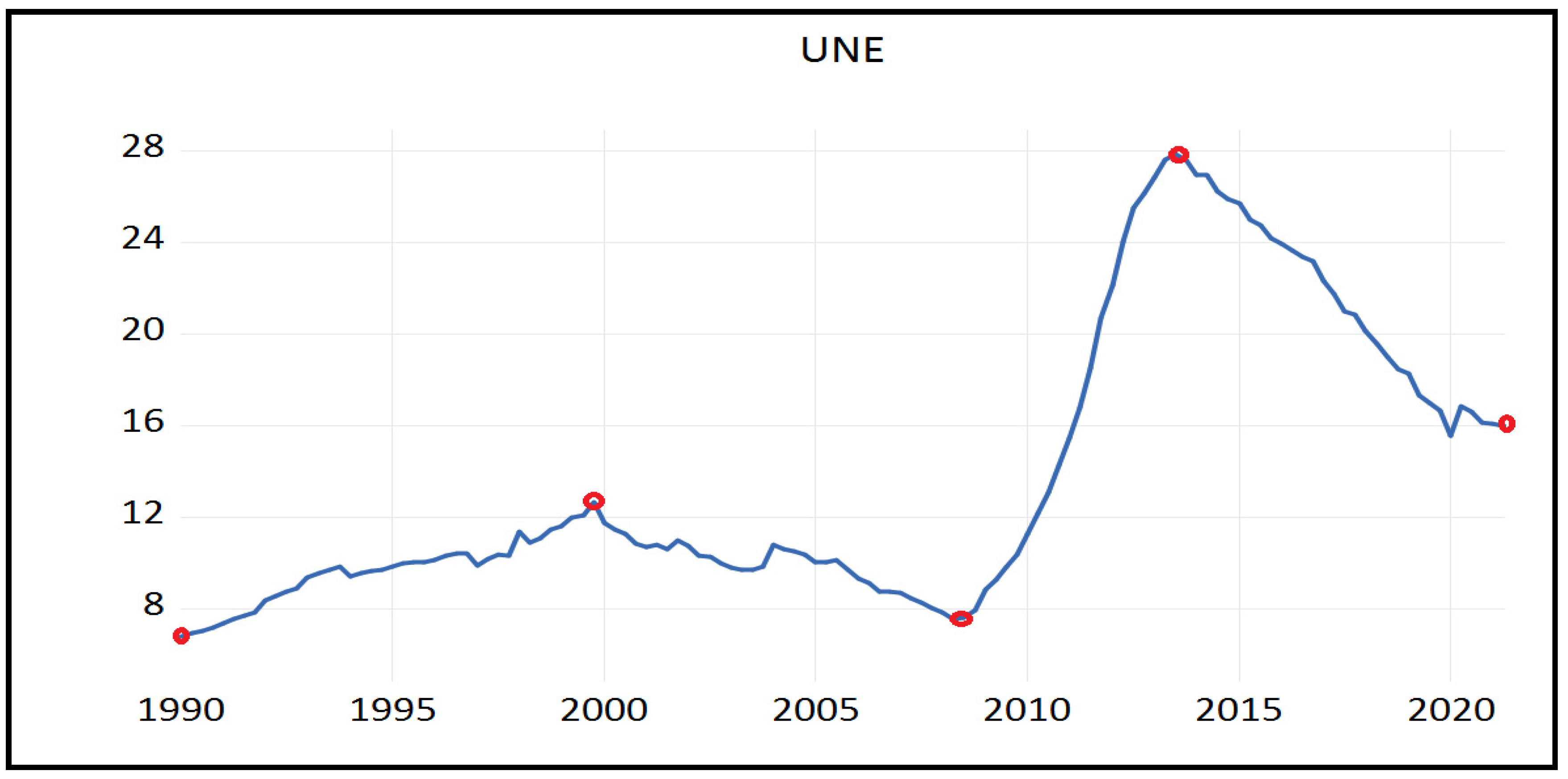
For the analysis of our paper, seasonally adjusted quarterly data are used for unemployment (UNE) from the first quarter of 1990 until the second quarter of 2021.

Given that the seasonal variance does not contaminate the cyclical signal, the HP filter should be applied in seasonally adjusted series. As it is referred to in [24], the presence of higher transitory noise on seasonally adjusted series can contaminate the cyclical signal and its extraction may be suitable. Excluding the seasonal effect, we could make useful comparisons between the observations. Moreover, the seasonal adjustment tends to smooth a data series, allowing data users to observe the changes in trend easier. The data source is the Federal Reserve Bank of St. Louis.

Analyzing the Data

The first step into data analysis is using graphs. The graph below presents seasonally adjusted quarterly data for unemployment in Greece.

Looking at Figure 1, we could conclude that unemployment occurs in four periods. The first period shows an increasing trend from 1990Q1–1999Q4 which is due to the continued shrinking of the agricultural sector, as well as the sharp growth of the labour force, in which women were extended participation in the workforce, and the immigrant inflow contributed, with the turning point being in 1999Q4. The second period involves a downward trend from 2000Q1 until 2008Q2, which is attributed to the common European currency, the Euro, with the turning point being in 2008Q2. The third period includes a sharp increasing trend from 2008Q3 to 2013Q3, with the turning point occuring in 2013Q3. The great increasing trend of unemployment since the beginning of 2008 is due to the global financial crisis as well as the debt crisis in Greece. The fourth period shows a decreasing trend in unemployment from 2013Q4 to 2021Q2, due to the support of Greek economy which came from the Eurozone summit for employment and development, with a turning point in 2021Q2. In addition, looking at the graph, one could observe that since the Greek crisis of 2013, the 2021 unemployment rate has reverted to the debt crisis rate.

5. Results

The current section compares the filtered series using the HP with the ones using regression, using real data in order to highlight the impact of filters in applied research. More specifically, we apply filters in the case of unemployment in Greece. Compared with the properties of big samples, we add the implications of small filter samples which become relevant in this empirical exercise.

Table 1. Descriptive statistics.

	Standard Deviations
Filter	A	B	C	D	Full
HP (1600)	0.307	0.367	1.063	0.477	1.205
HF (2-year regression)	0.545	0.789	1.310	0.841	2.486
	First-order autocorrelations
HP (1600)	0.262	0.260	0.469	0.398	0.386
HF (2-year regression)	0.289	0.268	0.222	0.455	0.575

Notes: A–D denotes the four sample periods. HF depicts the Hamilton filter and HP depicts the Hodrick–Prescott filter. Bold numbers indicate significance at least at the 5% level.

presents the descriptive statistics such as standard deviations and first order autocorrelations for the four periods separately, as well as the whole sample.

As suggested from the power transfer functions and as claimed by [8], the detrended series of the Hamilton two-year regressed series have greater volatility compared to those filtered with HP (1600) in all periods under investigation. Table 1 and all figures presented later, show that the historic volatility of two-year unemployment filtered with regression is more than double the filtered series using HP (1600) (2.486 compared to 1.205 in the whole sample), as well as the other sample periods under examination. Even the first order autoregressions of the detrended indicators range from 0.386 to 0.575 (see Table 1)

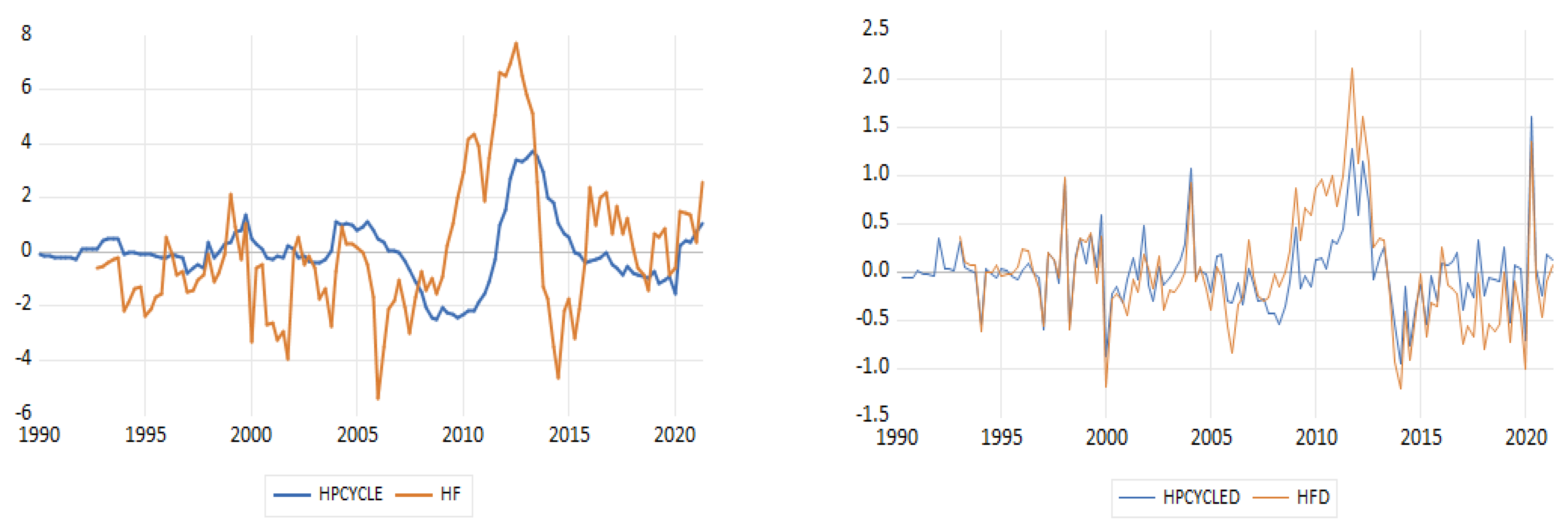
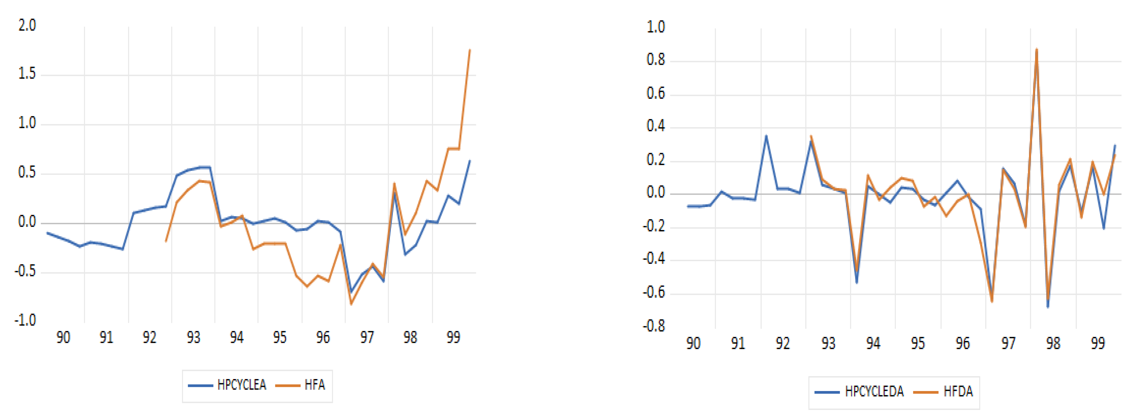
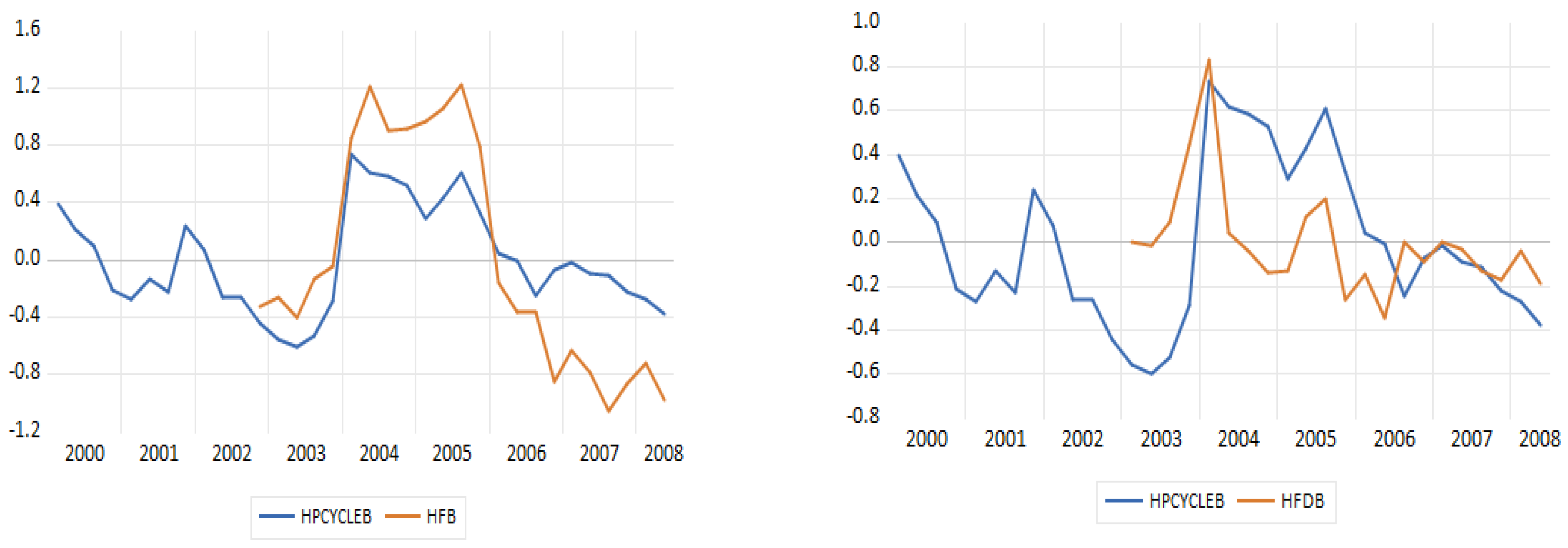
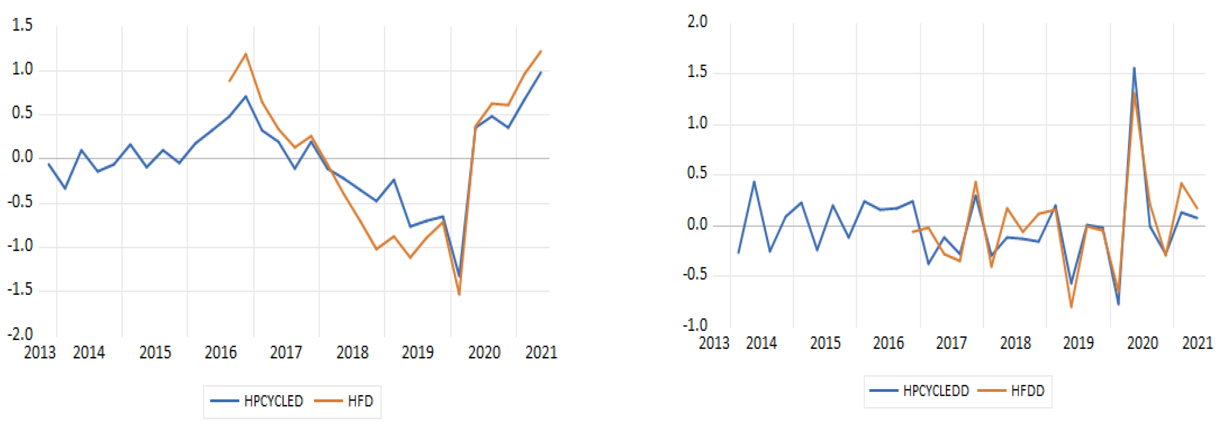
The Figure 2, Figure 3, Figure 4, Figure 5 and Figure 6 present the detrended series detected through the HP filter (1600) (in blue) and those detected through the Hamilton two-year regression filter (in brown) that regresses every variable with t + 8 in four more recent values of t, with the standard deviations and first order regressors for all periods.

In all periods depicted in the figures, as well as the first order autoregressions, we observe that the volatility of the two-year filtered regressed unemployment is bigger than the HP filtered series (1600). Due to the fact that the two-year Hamilton filter puts emphasis on the frequencies that are bigger than the typical frequencies of a business cycle (longer than eight years) and cancels fluctuations in a period of approximately two years, it does not record all phases that are classified by the National Bureau of Economic Research’s Business Cycle (NBER) (see [29]). This can be shown in basic terms when examining the series of the whole sample with the unemployment regression. It does not imply the quick contraction and recovery around the Greek debt crisis of 2013; on the contrary, it indicates a prolonged contraction. Cycle reinforcement is bigger than typical business cycles and seems to be more important than the periods under examination in terms of the whole sample. Moreover, as seen in the figure of the whole sample, cycles have a smaller duration for the two-year Hamilton regression filter than the cycles of the HP filter, as the series with the decreased two-year regression filter trend, show a larger volatility than the series HP filter (1600). Unemployment phase classification is mainly determined by the medium-term cycles. Moreover, at the first order autocorrelations, detrended indicators are smaller than those of standard deviations in all samples and fluctuate between 0.386 and 0.575 (see Table 1).

Nevertheless, the characteristics of the frequencies sector of the HP filter, have the following consequences:

• Cycle volatility is controlled from the smoothing parameter $\lambda$. Nevertheless, as $\lambda$ determines the volatility trend, there is no way to model the trend and the cycle independently from each other. The extraction of smaller cycles come automatically with a cost of a more imbalanced trend.
• In the model where the cycle component is absent, there are significant consequences when the model is processed with newly added data at the end of the sample. There is no other option than allocating the information, including the new data, either in the trend or the cycle, despite them not representing a outlier which is not due to the date process under the HP filter.

6. Forecasting Process

As mentioned before, the HP filter is a linear trend filter with time variable weights. De Jong and Sakarya [38] show that although weights at both ends of the series are always volatile through time, those at the body for the series are timely invariable, provided that the time series is big enough and $\lambda$ = 1600. Those time-invariable weights define the central HP filter, which is a symmetrical, non-negative specified, moving average filter (type 2) whose weights can be found in [8].

$$w(s)=\frac{1}{\alpha }\sin (\left|s\right|\vartheta +\varphi ){\rho }^{\left|s\right|}$$

(22)

where

$$\rho =\frac{1}{\sqrt{1+\delta }+\sqrt{\delta }}$$

with

$$\delta =\frac{1+\sqrt{1+16\lambda }}{8\lambda }$$

$$\alpha =\sqrt{\lambda \left({\rho }^2+\frac{1}{{\rho }^2}-2\cos 2\vartheta \right)}$$

with

$$\vartheta ={\tan }^{-1}\left(\frac{1}{2\lambda }\frac{1+{\rho }^2}{1-{\rho }^2}\right)$$

and

$$\varphi ={\tan }^{-1}\left(2\sqrt{\lambda }{(\tan \vartheta )}^2\right)$$

This is the central HP filter which we adopt as a trend filter.

The within sample prediction is a formal evaluation process of the prognostic opportunities of the models which were developed using observed data in order to see how efficient the algorithms are in terms of data reproduction. It is similar to a mechanic learning algorithm.

We have mentioned before, that in a time series $g_t$, the HP filter calculates the coordinates of trend $g_t$ and cycle $c_t$ from optimising the function below:

$$\underset{(g_t)\underset{t=1}{T}}{\min }\left({\displaystyle \sum _{t=1}^T{(y_t-g_t)}^2+\lambda {\displaystyle \sum _{t=3}^T{({\mathrm{\Delta }}^2{g}_t)}^2}}\right)$$

(23)

where Δ is the differentiation operator and $\lambda$ is a coordination parameter. If we suppose that the coordinates of $g_t$ and the trend and cycle of $c_t$ have been calculated for the HP filter, and we wish to forecast the next out of sample observation $y_{t+1}$.

According to (1) we will have:

$$y_{t+1}=g_{t+1}+c_{t+1}$$

(24)

Therefore, based on the function above, we should forecast the coordinates of trend $g_{t+1}$ and cycle $c_{t+1}$. The cycle coordinate can be predicted through the dynamic model which will possibly adjust to $\left\{c_t\right\}\underset{t=1}{T}$. As far as the trend coordinate is concerned, it could not be predicted from minimising the function. The only way we could use the HP filter for forecasting is for it to be applied to the ex post forecast, to a big data set $\left\{y_t\right\}\underset{t=1}{T+1}$ and then predict the trend coordinate $\left\{g_t\right\}\underset{t=1}{T+1}$ and the cycle coordinate $\left\{c_t\right\}\underset{t=1}{T+1}$.

As a result, the characteristics of the frequency of the HP filter, have the following consequences:

• Cycle volatility is being tested from the smoothing parameter. Nevertheless, as Function (23) defined the trend-imbalance, there is no way to model the trend and the cycle independently. The extraction of smaller cycle becomes automatic to the cost of a more imbalance trend.
• The model from which the cycle coordinate is missing, has significant implications when additional data are submitted at the end of the sample.
• The irregular random effects are absent from the HP filter model. This tends to increase the imbalance of the trend estimation in real time as the random effects are forced to partly contribute to the variability of the trend.

Moreover, in order to forecast unemployment, we adopt the Hamilton method as a strong autoregressive forecasting which yields stable predictions $y_t$ for a wide variety of non-stationary procedures. In essence, Hamilton avoids the Model (2) framework with the appropriate trend of $g_t$ and trend deviation $c_t$. On the contrary, he argues that information coming from an economic cycle could be collected directly from time series y_t using suitably chosen OLS prediction errors.

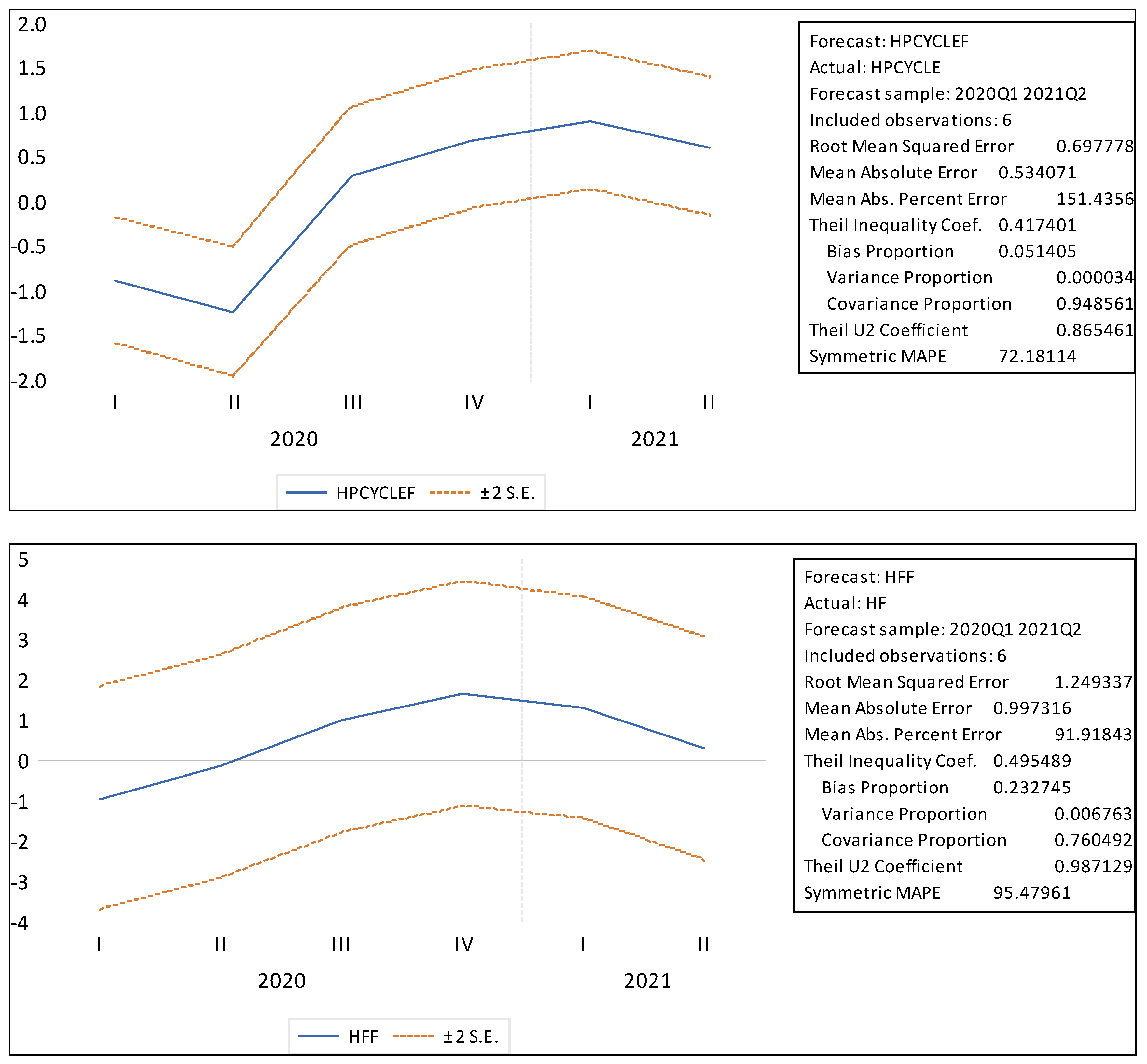
Figure 7 show the dynamic forecasting of unemployment, as well as the estimation indices of forecasting, such as RMSE (Root Mean Squared Error), MAE (Mean Absolute Error), MAPE (Mean Absolute Percentage Error), and Theil Inequality Coefficient.

The precision of these forecasts is closely related to the quality of filter trends which are associated to the extension of predictions.

At the prediction environment for six quarters (2020Q1–2021Q2), the HP filter gives better returns compared to Hamilton’s two-year regression filter. These findings are in line with the most extended theoretical and practical data from the literature review around predictions–extensions. In order to analyse the macroeconomic economic cycle, the optimum prediction extension should be used regularly to minimise the trend imbalance around the ends of the series. As a rule of thumb, the more accurate the prediction extension, the more precise and accurate, but less imbalance is the trend of the extension of HP prediction at the end. Finally, looking at the figure above, we observe that the dynamic prediction of the HP filter is better than that of Hamilton in all estimation indices. More specifically, the predictive ability of a model is significant when bias proportion and variance proportion are small, so more prediction errors correspond to a covariance proportion, meaning that it corresponds to a non-systematic prediction error.

7. Conclusions

The current paper investigated whether the use of Hamilton’s regression filter significantly alters unemployment cycles in the case of Greece, in comparison to those derived from the double Hodrick–Prescott (HP) filter. Hamilton [1] proposes the use of a single regression filter so as to overcome some of the disadvantages of the HP filter, such as the presence of dummy cycles, the bias at the sample end, and the ad hoc hypotheses for soothing parameters. As the literature review suggests, the HP filter remains a widely used technique for business cycles and for decomposing economic analysis. This is usually the method used to be compared to other methods. This is also the case in the current paper where unemployment in Greece is being examined.

The macroeconomic time series that we use in this paper (seasonally adjusted) is decomposed in an element that records a trend, which presents some sort of flexibility or break, and also a cyclical component which is stationary. An important issue that arises when discussing a specific method, compared with alternative approaches, is the question about what a “trend” is called. Sometimes, on empirical papers, this concept is not mentioned, and thus its results are not challenged. So, it is useful from this point of view to be aware of the discrimination between trend, stationarity, and stochastic trend [35]. The concept of “trend” is usually referred to as a deterministic trend or as a trend that is influenced by exogenous shocks that provide transitory results. In our paper, the trend is developed smoothly, apart from some breaks, which are referred to economic facts. Trend estimation methods consist of moving average filters modifying the dynamic structure of the first time series, and providing steady estimations of the historical series trend. The reference on “stochastic trends” is based mainly on the hypothesis that they follow a random walk. In such cases, these shocks have permanent effects on the trend. A similar case can occur in the cyclical component so we can assume that we have stochastic phenomena [35].

Using a number of quarterly data for unemployment in Greece for a macroeconomic soothing model, we showed that trend and cycle coordinates of the filter for Hamilton regression leads to significantly larger cycle volatilities than those derived from the HP filter. As a consequence, mainly based on the fact that the Hamilton filter produces substantially larger volatilities and less reliable trends that move mainly during significant economic periods, such as the Greek debt crisis in 2013, we have a clear preference for economic cycle measures which are obtained from the HP filter and not from the Hamilton filter process.

The forecast of a sample is also a process of estimating the prognostic potential of the model developed based on the observed data in order to see how effective algorithms are made into reproducing data. Hamilton’s methodology as a powerful autoregressive prediction which yields constant predictions for a wide variety of non-stationary procedures, as well as the HP filter, has been used to forecast the ex post prediction on a number of unemployment data in the case of Greece.

For macroeconomic data of an open economy, we conclude that the HP filter remains our method of choice for analysing the decomposition of a time series. With this established, we use HP predictions in order to tackle widely acknowledged limitations of the HP filter at the end of the series.

As Hodrick suggests in his paper in 2020 [31], a future paper for researchers can focus on the development of simultaneous multivariate econometric models that can apply filters for the decomposition of a trend component and a cyclical component that exist in economic data, and drive business cycles’ development.