
Performance of Dense Wireless Networks in 5G and beyond Using Stochastic Geometry


Abstract
:1. Introduction
2. System Model
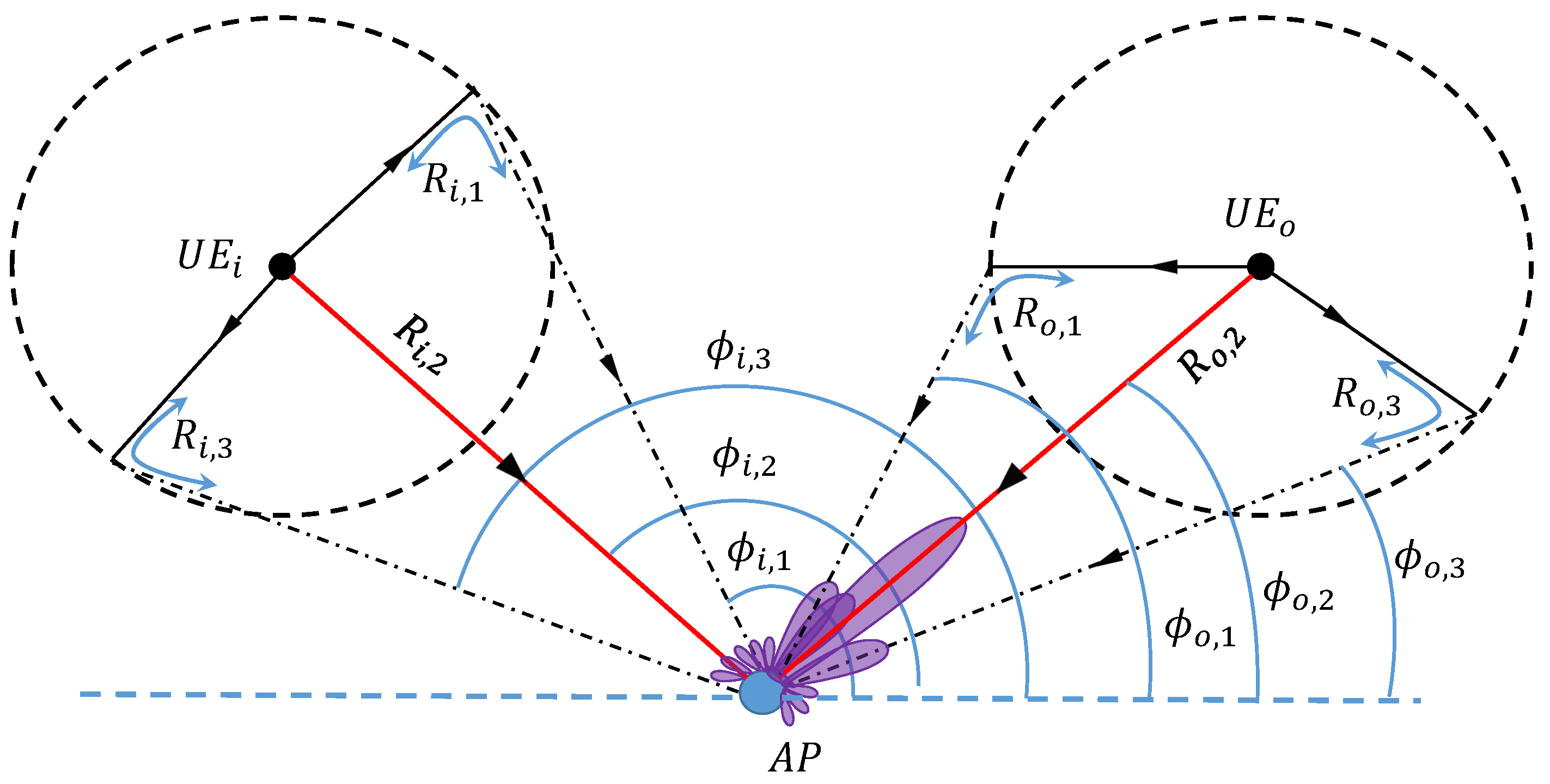
2.1. Array Gain Model
2.2. Signal Model and Service Probability
3. CF of the Aggregated Interference in LOS
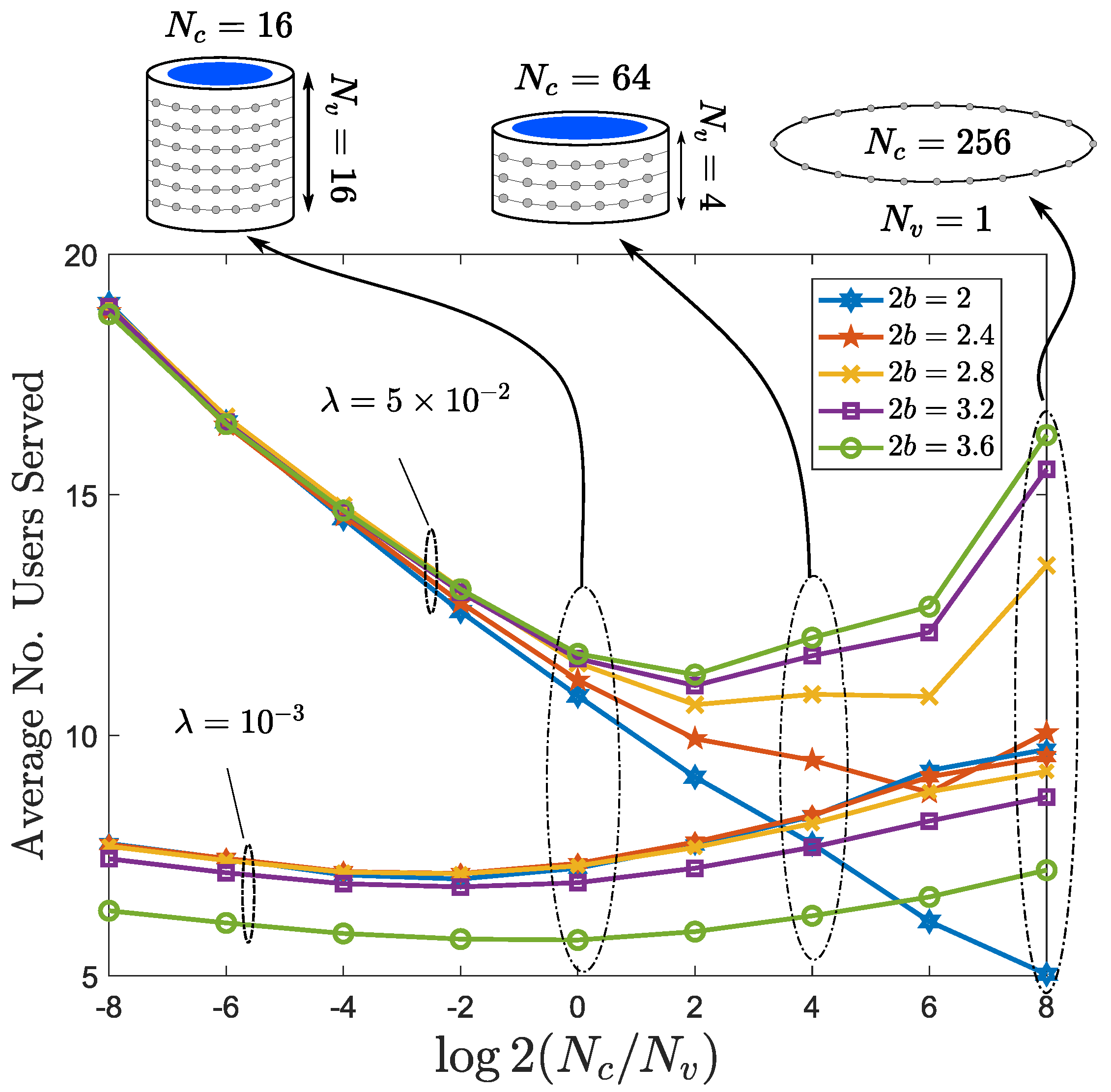
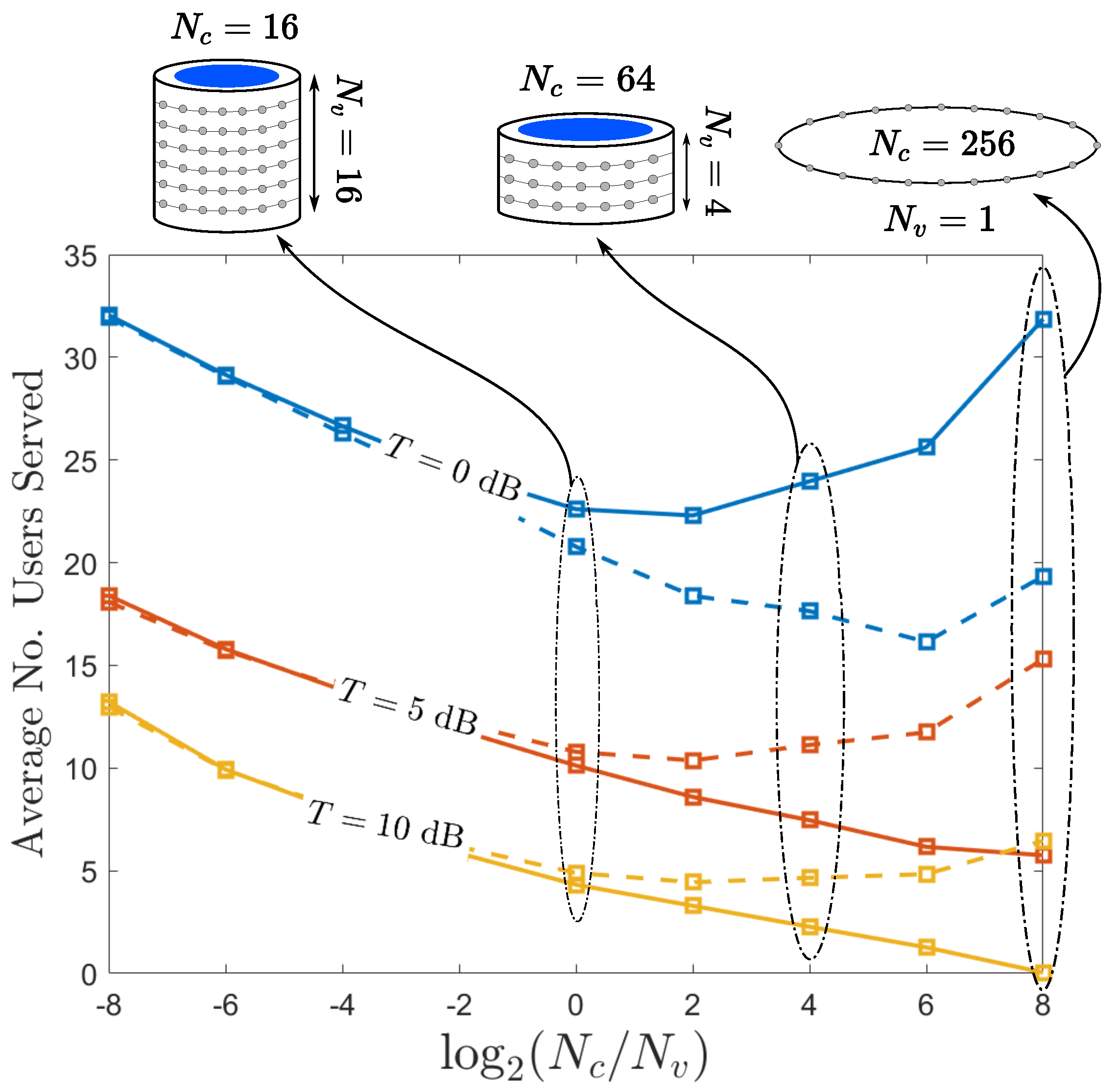
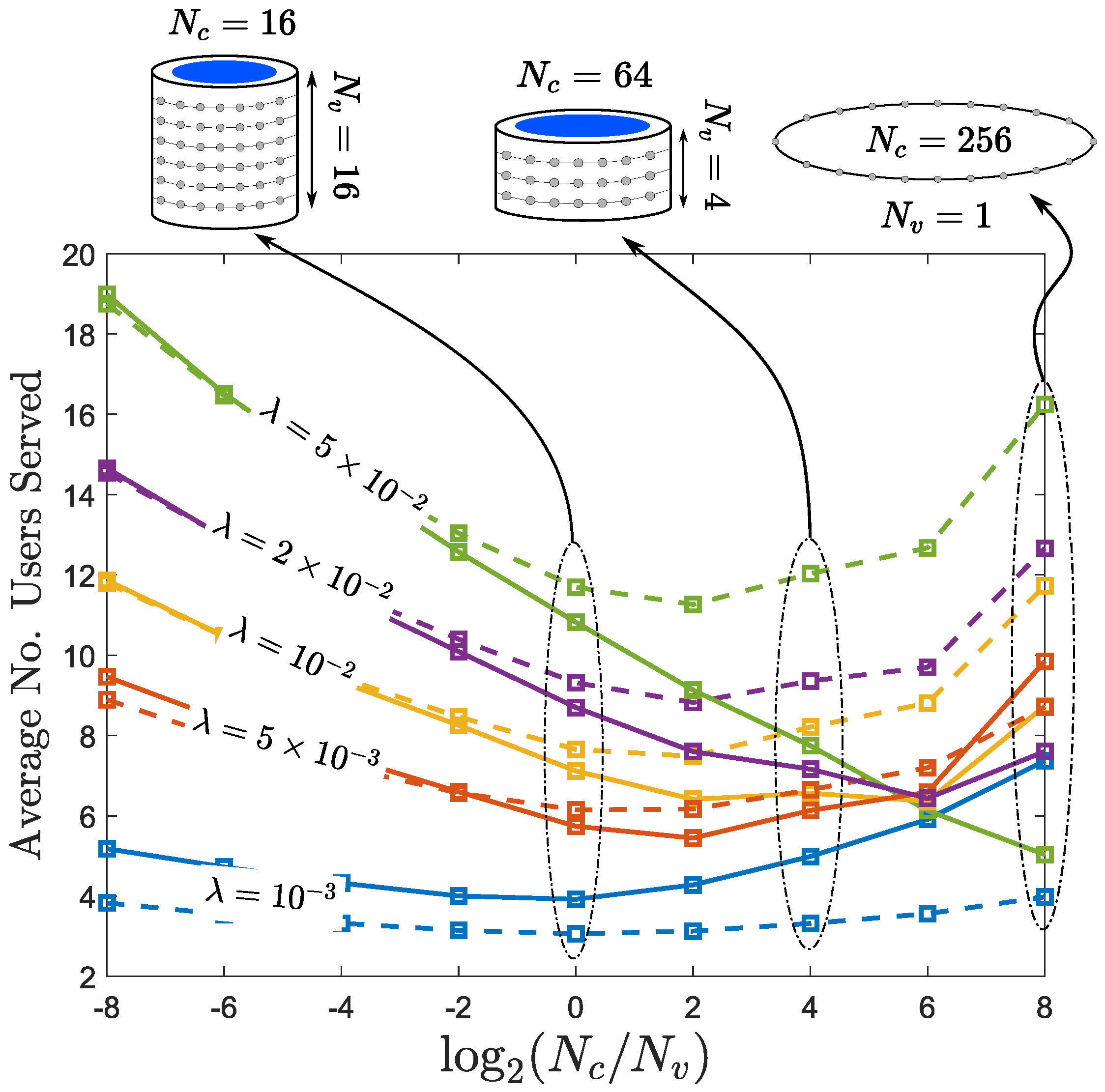
3.1. Uniform Cylindrical Arrays
3.2. Specific Cases
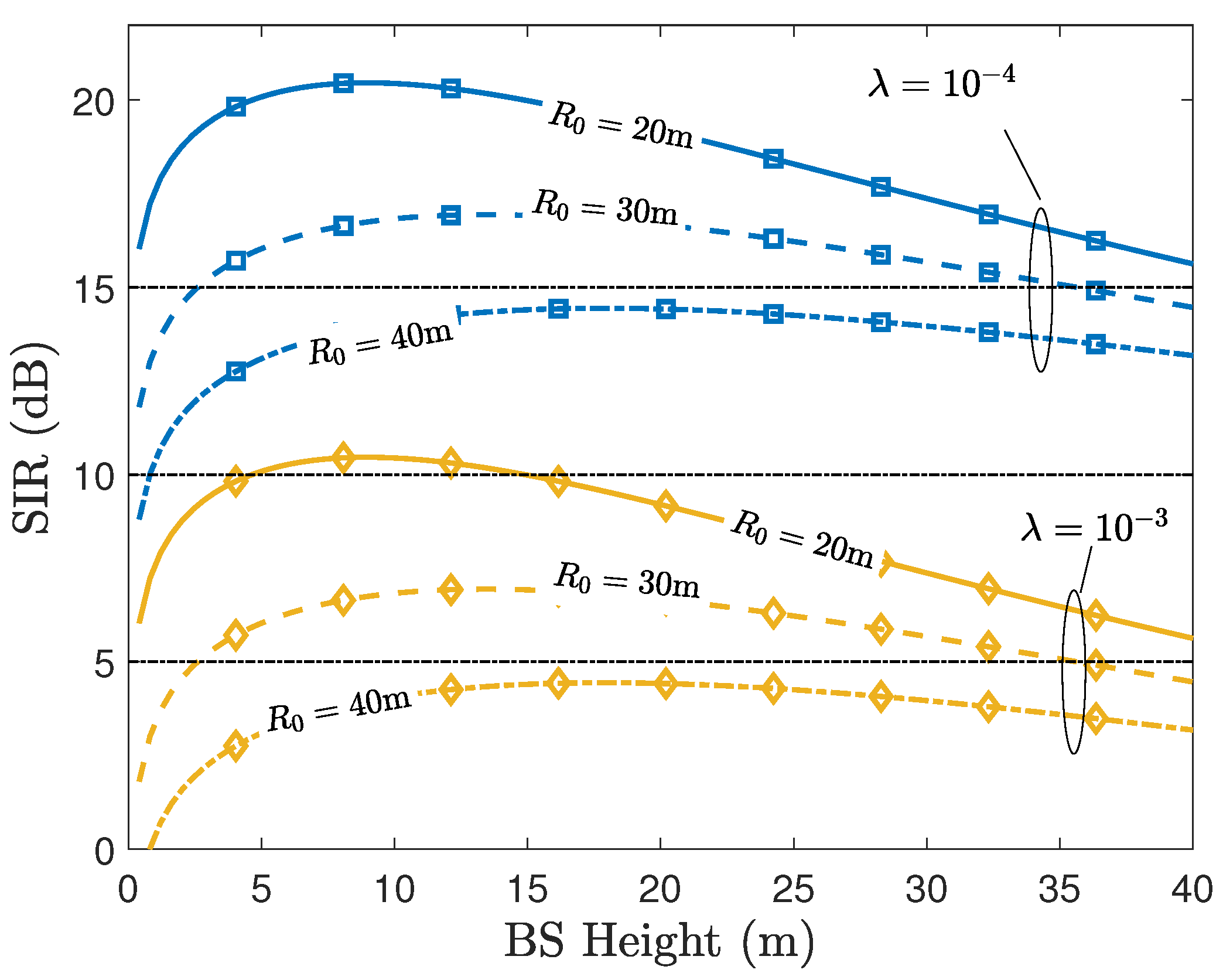
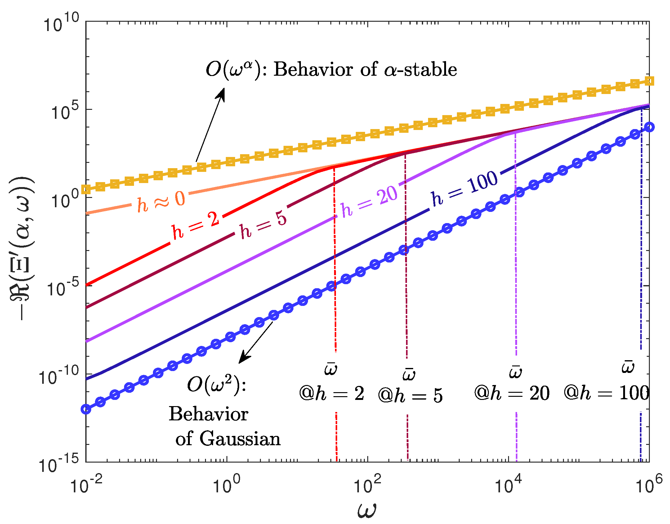
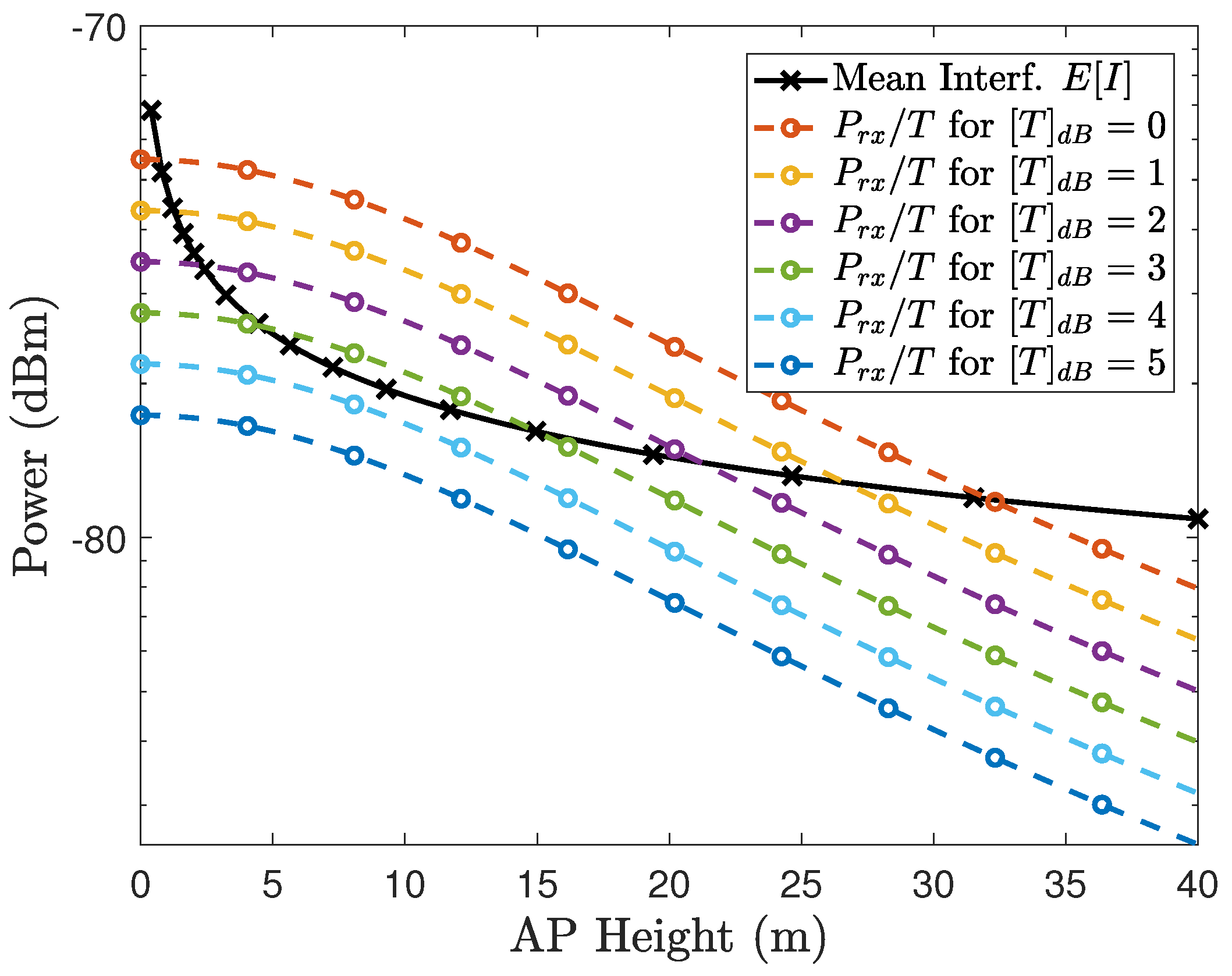
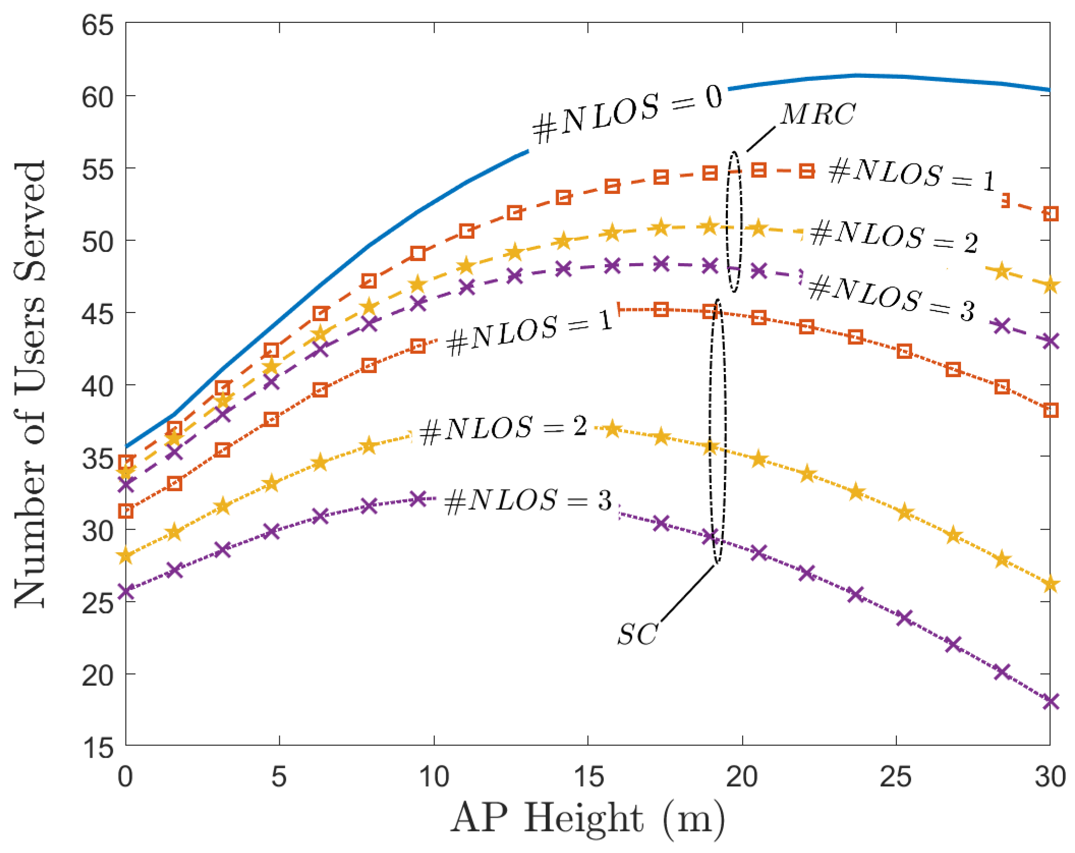
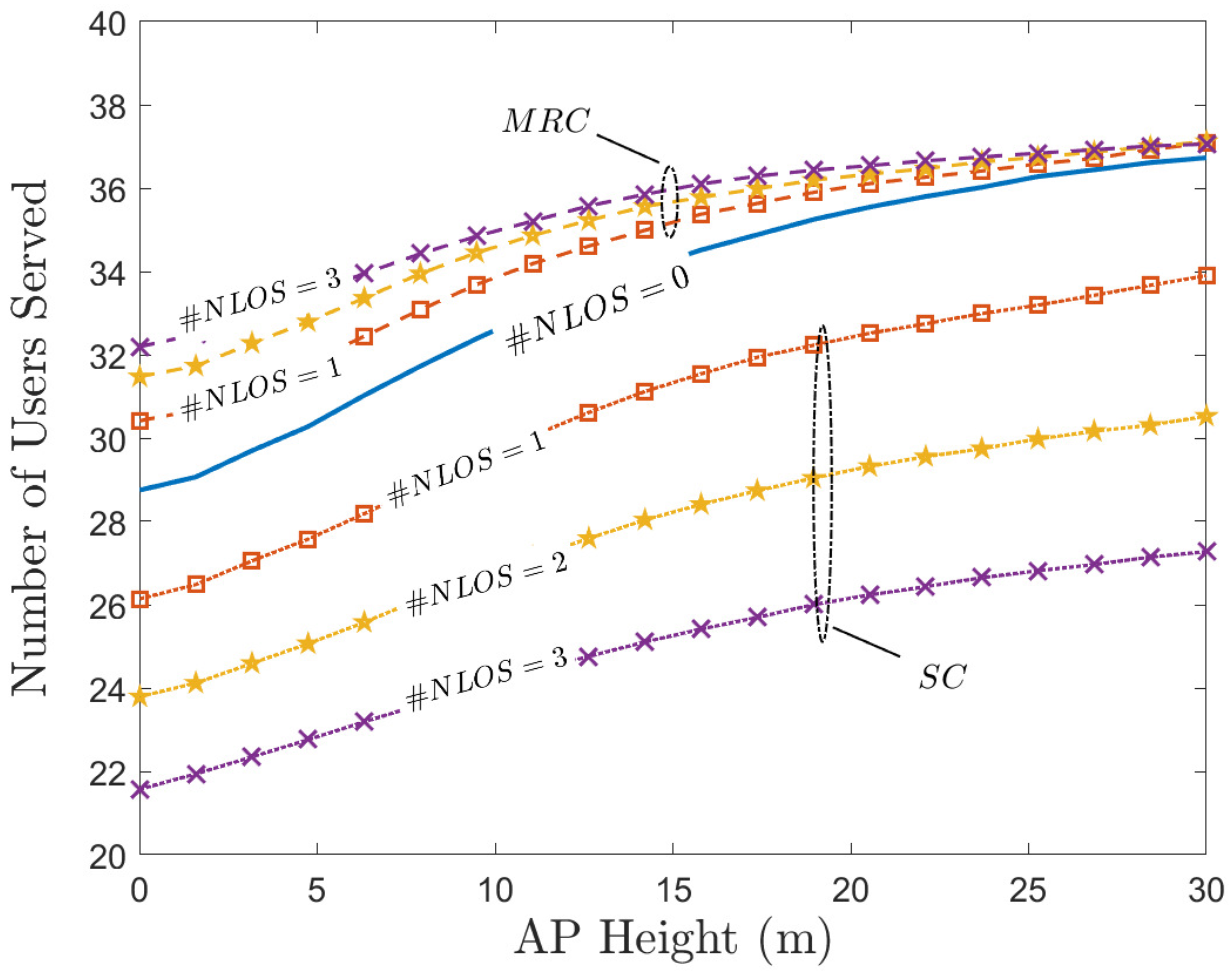
3.3. Analysis of AP Height
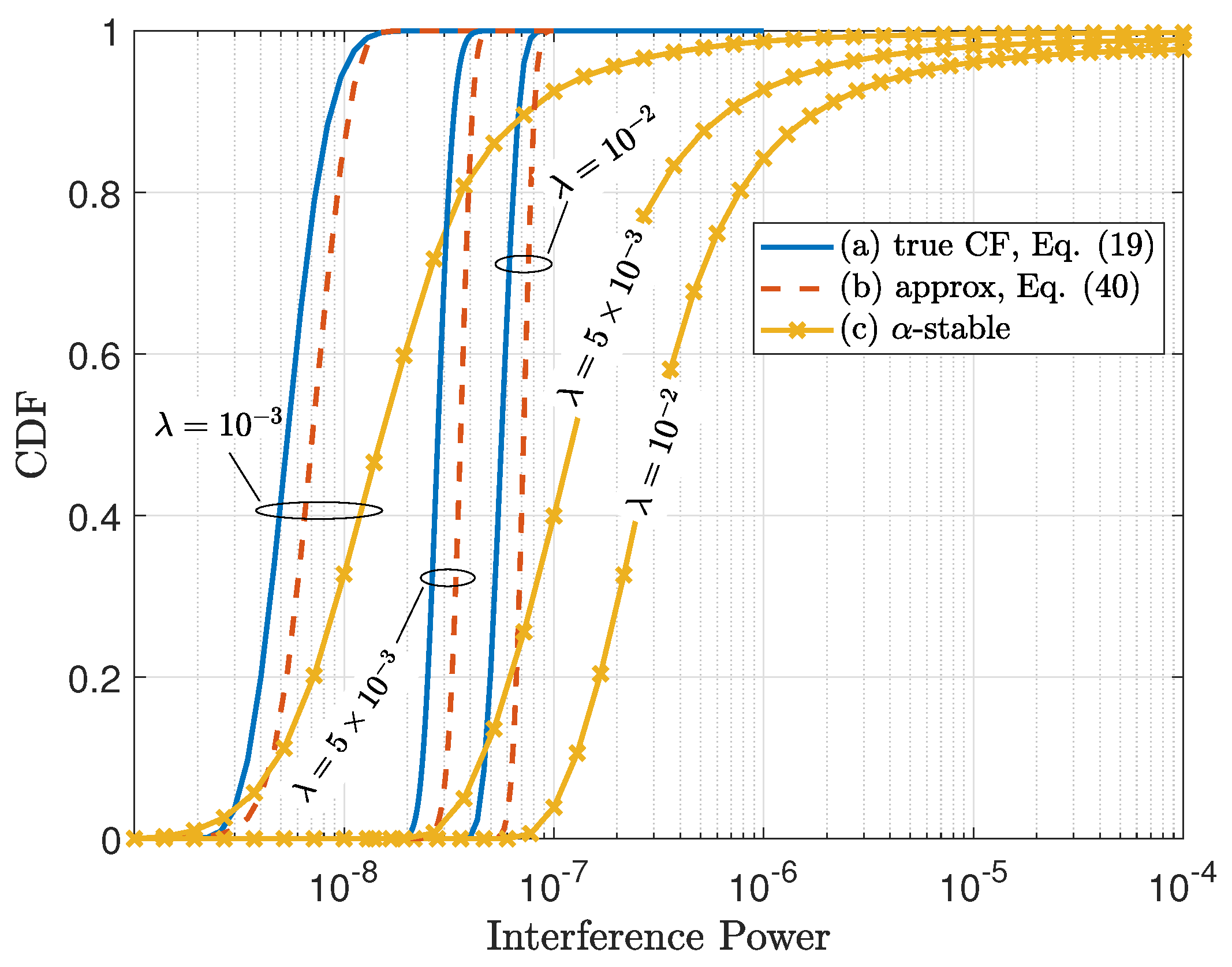
3.4. Numerical Validation on Aggregated Interference
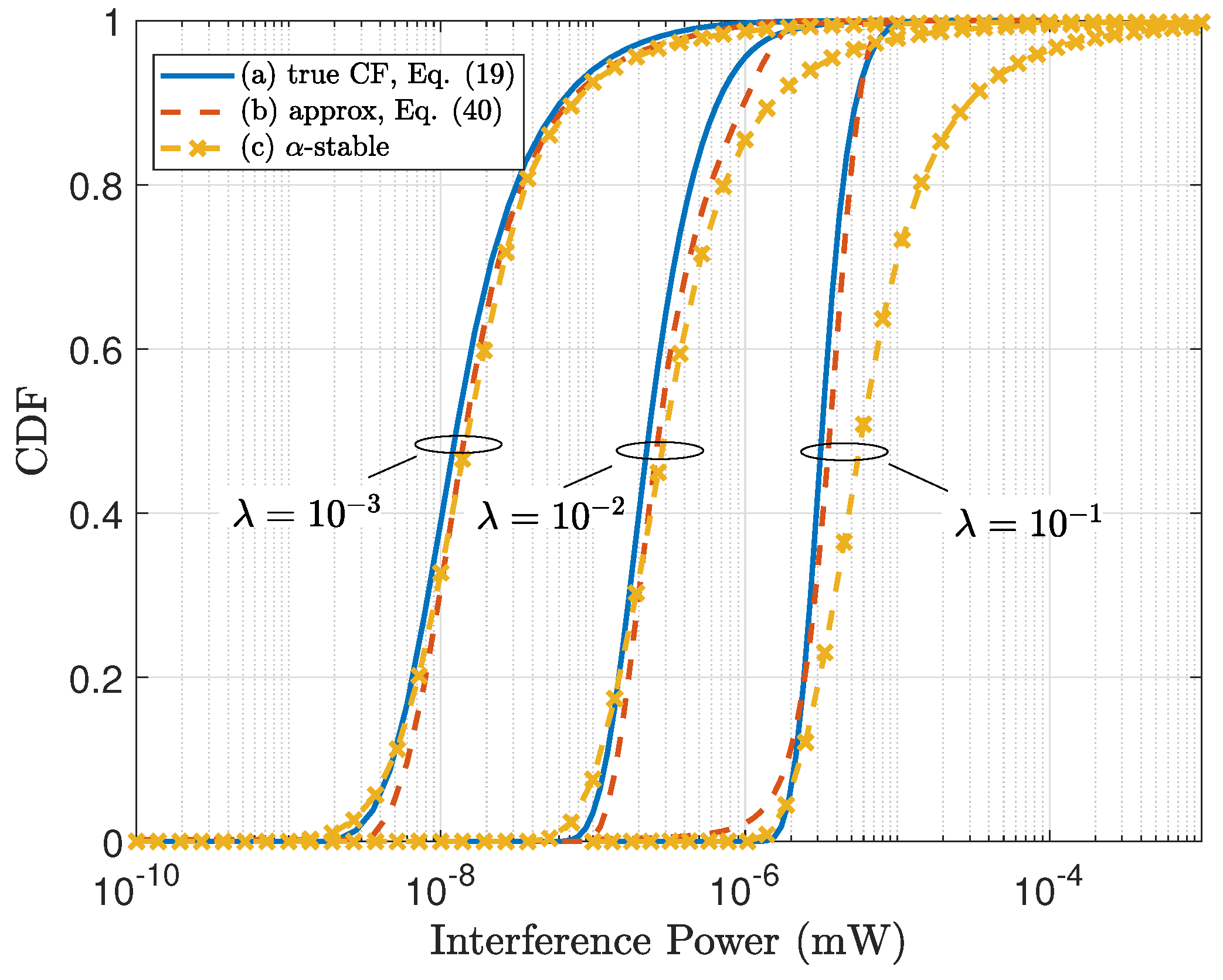
4. Statistical Characterization of the Aggregated Interference Power
5. Outage Analysis in the Presence of NLOS, Noise and Blockage
5.1. NLOS Paths
5.2. NLOS Paths
5.3. Noise
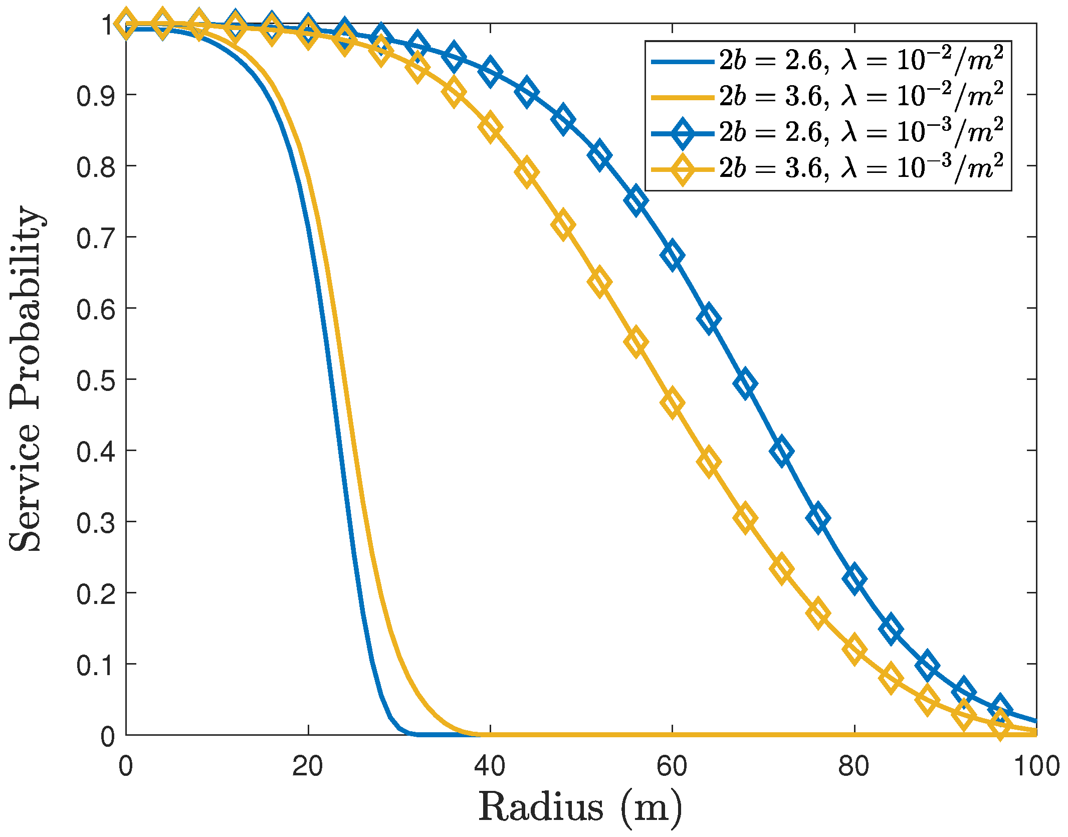
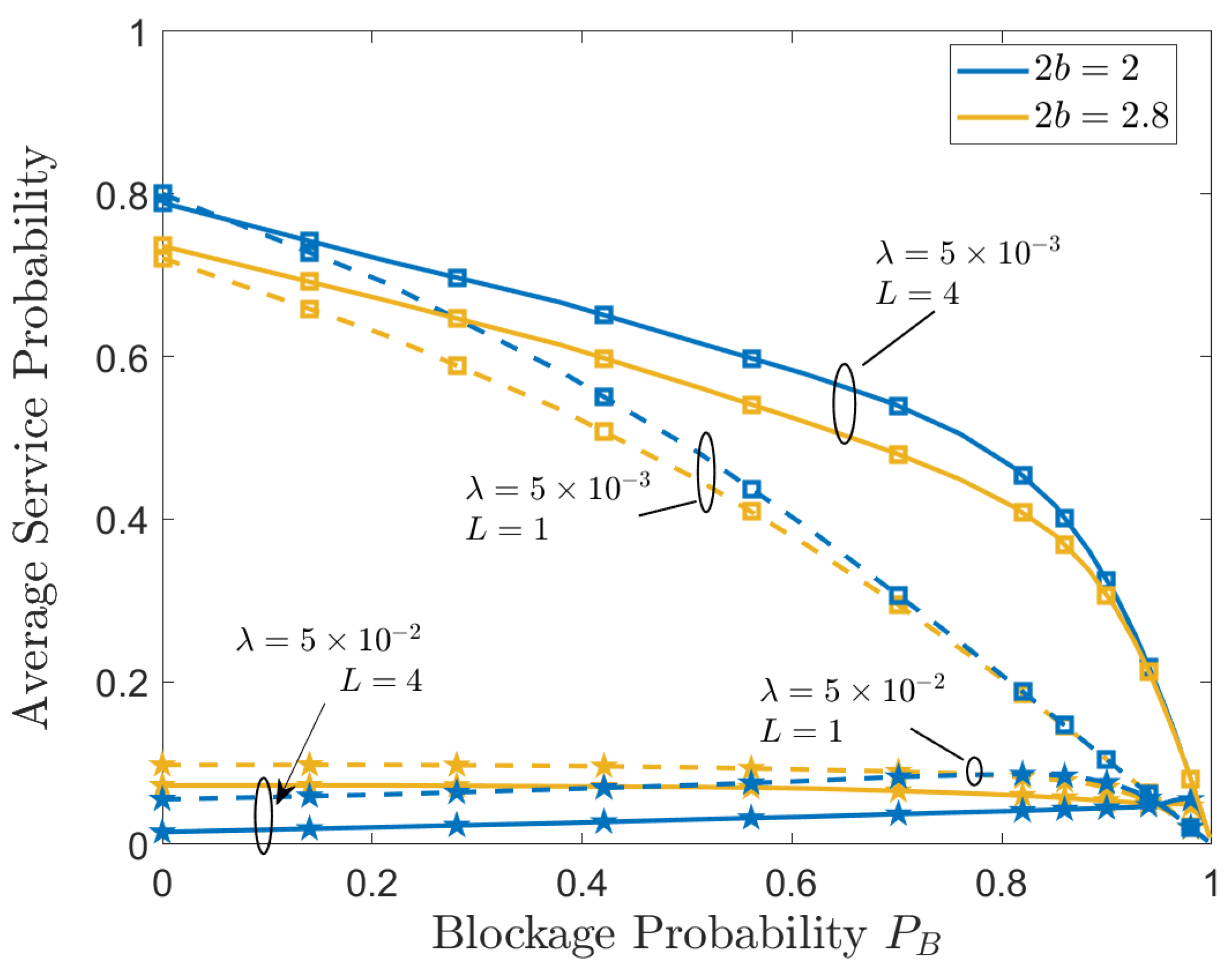
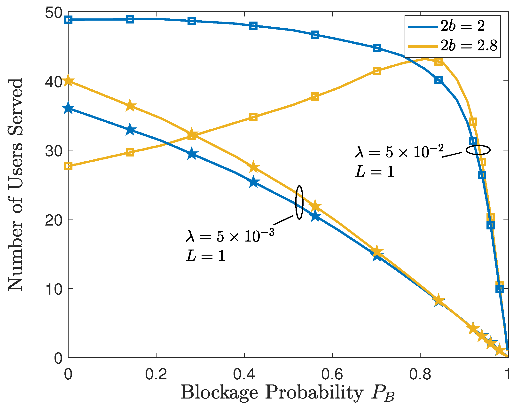
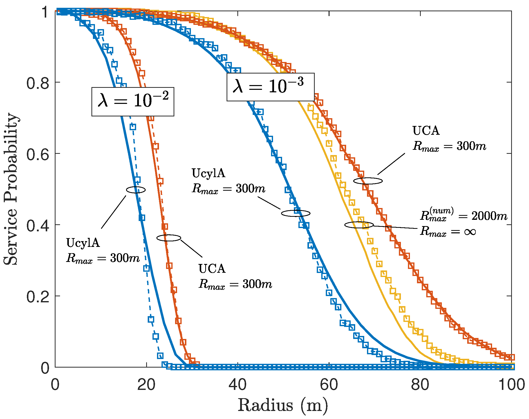
5.4. Blockage
6. Conclusions
Author Contributions
Funding
Institutional Review Board Statement
Informed Consent Statement
Conflicts of Interest
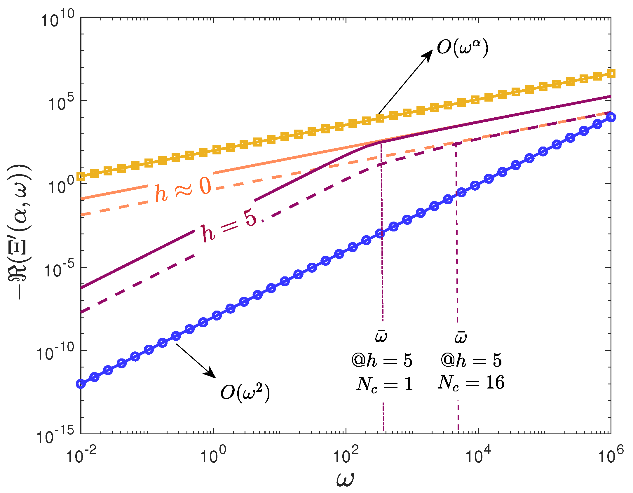
Appendix A. Singularity Point
Appendix B. Derivative of Mean Aggregated Interference
Appendix C. Proof of MRC
Appendix D. Multipath Interference
References
- Panwar, N.; Sharma, S.; Singh, A.K. A survey on 5G: The next generation of mobile communication. Phys. Commun. 2016, 18, 64–84. [Google Scholar] [CrossRef] [Green Version]
- Rappaport, T.T.S.; Sun, S.; Mayzus, R.; Zhao, H.; Azar, Y.; Wang, K.; Wong, G.N.; Schulz, J.K.; Samimi, M.; Gutierrez, F. Millimeter Wave Mobile Communications for 5G Cellular: It Will Work! IEEE Access 2013, 1, 335–349. [Google Scholar] [CrossRef]
- Qamar, F.; Siddiqui, M.U.A.; Hindia, M.N.; Hassan, R.; Nguyen, Q.N. Issues, Challenges, and Research Trends in Spectrum Management: A Comprehensive Overview and New Vision for Designing 6G Networks. Electronics 2020, 9, 1416. [Google Scholar] [CrossRef]
- Azpilicueta, L.; Lopez-Iturri, P.; Zuñiga-Mejia, J.; Celaya-Echarri, M.; Rodríguez-Corbo, F.A.; Vargas-Rosales, C.; Aguirre, E.; Michelson, D.G.; Falcone, F. Fifth-Generation (5G) mmWave Spatial Channel Characterization for Urban Environments’ System Analysis. Sensors 2020, 20, 5360. [Google Scholar] [CrossRef] [PubMed]
- Ikram, M.; Sultan, K.; Lateef, M.F.; Alqadami, A.S.M. A Road towards 6G Communication; A Review of 5G Antennas, Arrays, and Wearable Devices. Electronics 2022, 11, 169. [Google Scholar] [CrossRef]
- Singh, R.; Lehr, W.; Sicker, D.; Huq, K. Beyond 5G: The Role of THz Spectrum. In Proceedings of the TPRC47: The 47th Research Conference on Communication, Information and Internet Policy, Washington, DC, USA, 20–21 September 2019. [Google Scholar] [CrossRef]
- Dong, K.; Mizmizi, M.; Tagliaferri, D.; Spagnolini, U. Vehicular Blockage Modelling and Performance Analysis for mmWave V2V Communications. arXiv 2021, arXiv:2110.10576. [Google Scholar]
- Ngo, H.Q.; Larsson, E.G.; Marzetta, T.L. Energy and Spectral Efficiency of Very Large Multiuser MIMO Systems. IEEE Trans. Commun. 2013, 61, 1436–1449. [Google Scholar] [CrossRef] [Green Version]
- Ojo, M.O.; Aramide, O.O. Various interference models for multicellular scenarios: A comparative study. In Proceedings of the 2015 Fifth International Conference on Digital Information and Communication Technology and Its Applications (DICTAP), Beirut, Lebanon, 29 April–1 May 2015; pp. 54–58. [Google Scholar] [CrossRef]
- Ilow, J.; Hatzinakos, D. Analytic alpha-stable noise modeling in a Poisson field of interferers or scatterers. IEEE Trans. Signal Process. 1998, 46, 1601–1611. [Google Scholar] [CrossRef]
- Win, M.Z.; Pinto, P.C.; Shepp, L.A. A Mathematical Theory of Network Interference and Its Applications. Proc. IEEE 2009, 97, 205–230. [Google Scholar] [CrossRef]
- Clavier, L.; Pedersen, T.; Larrad, I.R.; Egan, M. Alpha-Stable model for Interference in IoT networks. In Proceedings of the 2021 IEEE Conference on Antenna Measurements Applications (CAMA), Antibes, France, 15–17 November 2021; pp. 575–578. [Google Scholar] [CrossRef]
- Clavier, L.; Pedersen, T.; Larrad, I.; Lauridsen, M.; Egan, M. Experimental Evidence for Heavy Tailed Interference in the IoT. IEEE Commun. Lett. 2021, 25, 692–695. [Google Scholar] [CrossRef]
- Mukasa, C.; Aalo, V.A.; Efthymoglou, G. Exact distributions for aggregate interference in wireless networks with a poisson field of interferers. In Proceedings of the 2016 IEEE 12th International Conference on Wireless and Mobile Computing, Networking and Communications (WiMob), New York, NY, USA, 17–19 October 2016; pp. 1–5. [Google Scholar] [CrossRef]
- Zheng, C.C.; Egan, M.; Clavier, L.; Pedersen, T.; Gorce, J.M. Linear combining in dependent α-stable interference. In Proceedings of the ICC 2020—IEEE International Conference on Communications, Dublin, Ireland, 7–11 June 2020. [Google Scholar]
- Hong, X.; Wang, C.X.; Thompson, J. Interference Modeling of Cognitive Radio Networks. In Proceedings of the VTC Spring 2008—IEEE Vehicular Technology Conference, Singapore, 11–14 May 2008; pp. 1851–1855. [Google Scholar] [CrossRef] [Green Version]
- ElSawy, H.; Sultan-Salem, A.; Alouini, M.; Win, M.Z. Modeling and Analysis of Cellular Networks Using Stochastic Geometry: A Tutorial. IEEE Commun. Surv. Tutor. 2017, 19, 167–203. [Google Scholar] [CrossRef] [Green Version]
- Baianifar, M.; Khavari, S.; Razavizadeh, S.M.; Svensson, T. Impact of user height on the coverage of 3D beamforming-enabled massive MIMO systems. In Proceedings of the 2017 IEEE 28th Annual International Symposium on Personal, Indoor, and Mobile Radio Communications (PIMRC), Montreal, QC, Canada, 8–13 October 2017; pp. 1–5. [Google Scholar] [CrossRef] [Green Version]
- Mouradian, A. Modeling dense urban wireless networks with 3D stochastic geometry. Perform. Eval. 2018, 121–122, 1–17. [Google Scholar] [CrossRef] [Green Version]
- ElSawy, H.; Hossain, E.; Haenggi, M. Stochastic Geometry for Modeling, Analysis, and Design of Multi-Tier and Cognitive Cellular Wireless Networks: A Survey. IEEE Commun. Surv. Tutor. 2013, 15, 996–1019. [Google Scholar] [CrossRef]
- Weber, S.; Andrews, J.G. Transmission capacity of wireless networks. arXiv 2012, arXiv:1201.0662. [Google Scholar]
- Bai, T.; Heath, R.W. Analyzing Uplink SINR and Rate in Massive MIMO Systems Using Stochastic Geometry. IEEE Trans. Commun. 2016, 64, 4592–4606. [Google Scholar] [CrossRef]
- Renzo, M.D.; Guidotti, A.; Corazza, G.E. Average Rate of Downlink Heterogeneous Cellular Networks over Generalized Fading Channels: A Stochastic Geometry Approach. IEEE Trans. Commun. 2013, 61, 3050–3071. [Google Scholar] [CrossRef] [Green Version]
- Filo, M.; Foh, C.H.; Vahid, S.; Tafazolli, R. Performance impact of antenna height in Ultra-Dense cellular Networks. In Proceedings of the 2017 IEEE International Conference on Communications Workshops (ICC Workshops), Paris, France, 21–25 May 2017; pp. 429–434. [Google Scholar]
- Liu, J.; Sheng, M.; Wang, K.; Li, J. The Impact of Antenna Height Difference on the Performance of Downlink Cellular Networks. arXiv 2007, arXiv:1704.05563. [Google Scholar]
- Al-Hourani, A.; Kandeepan, S.; Lardner, S. Optimal LAP Altitude for Maximum Coverage. IEEE Wirel. Commun. Lett. 2014, 3, 569–572. [Google Scholar] [CrossRef] [Green Version]
- Yoshikawa, K.; Yamamoto, K.; Nishio, T.; Morikura, M. Grid-Based Exclusive Region Design for 3D UAV Networks: A Stochastic Geometry Approach. IEEE Access 2019, 7, 103806–103814. [Google Scholar] [CrossRef]
- Azari, M.M.; Rosas, F.; Chiumento, A.; Pollin, S. Coexistence of Terrestrial and Aerial Users in Cellular Networks. In Proceedings of the 2017 IEEE Globecom Workshops (GC Wkshps), Singapore, 4–8 December 2017; pp. 1–6. [Google Scholar] [CrossRef] [Green Version]
- Chu, E.; Kim, J.M.; Jung, B.C. Interference modeling and analysis in 3-dimensional directional UAV networks based on stochastic geometry. ICT Express 2019, 5, 235–239. [Google Scholar] [CrossRef]
- Maamari, D.; Devroye, N.; Tuninetti, D. Coverage in mmWave Cellular Networks with Base Station Co-Operation. IEEE Trans. Wirel. Commun. 2016, 15, 2981–2994. [Google Scholar] [CrossRef]
- Cheng, M.; Wang, J.; Wu, Y.; Xia, X.; Wong, K.; Lin, M. Coverage Analysis for Millimeter Wave Cellular Networks with Imperfect Beam Alignment. IEEE Trans. Veh. Technol. 2018, 67, 8302–8314. [Google Scholar] [CrossRef] [Green Version]
- Andrews, J.G.; Baccelli, F.; Ganti, R.K. A Tractable Approach to Coverage and Rate in Cellular Networks. IEEE Trans. Commun. 2011, 59, 3122–3134. [Google Scholar] [CrossRef] [Green Version]
- Alwajeeh, T.; Combeau, P.; Vauzelle, R.; Bounceur, A. A high-speed 2.5D ray-tracing propagation model for microcellular systems, application: Smart cities. In Proceedings of the 2017 11th European Conference on Antennas and Propagation (EUCAP), Paris, France, 19–24 March 2017; pp. 3515–3519. [Google Scholar] [CrossRef]
- Liu, Z.; Guo, L.X.; Tao, W. Full automatic preprocessing of digital map for 2.5D ray tracing propagation model in urban microcellular environment. Waves Random Complex Media 2013, 23, 267–278. [Google Scholar] [CrossRef]
- Yu, X.; Zhang, J.; Haenggi, M.; Letaief, K.B. Coverage Analysis for Millimeter Wave Networks: The Impact of Directional Antenna Arrays. IEEE J. Sel. Areas Commun. 2017, 35, 1498–1512. [Google Scholar] [CrossRef]
- Josefsson, L.; Persson, P. Conformal Array Antenna Theory and Design; John Wiley & Sons: Hoboken, NJ, USA, 2006; Volume 29. [Google Scholar]
- Andrews, J.G.; Bai, T.; Kulkarni, M.N.; Alkhateeb, A.; Gupta, A.K.; Heath, R.W. Modeling and Analyzing Millimeter Wave Cellular Systems. IEEE Trans. Commun. 2017, 65, 403–430. [Google Scholar] [CrossRef] [Green Version]
- Stergiopoulos, S.; Dhanantwari, A.C. Implementation of adaptive processing in integrated active-passive sonars with multi-dimensional arrays. In Proceedings of the 1998 IEEE Symposium on Advances in Digital Filtering and Signal Processing. Symposium Proceedings (Cat. No.98EX185), Tokyo, Japan, 17 April 1998; pp. 62–66. [Google Scholar] [CrossRef]
- Razavizadeh, S.M.; Ahn, M.; Lee, I. Three-Dimensional Beamforming: A new enabling technology for 5G wireless networks. IEEE Signal Process. Mag. 2014, 31, 94–101. [Google Scholar] [CrossRef]
- Wu, N.; Zhu, F.; Liang, Q. Evaluating Spatial Resolution and Channel Capacity of Sparse Cylindrical Arrays for Massive MIMO. IEEE Access 2017, 5, 23994–24003. [Google Scholar] [CrossRef]
- Trees, H.L.V. Detection, Estimation, and Modulation Theory, Part III: Radar Sonar Signal Processing and Gaussian Signals in Noise; John Wiley & Sons, Inc.: Hoboken, NJ, USA, 2001. [Google Scholar]
- Spagnolini, U. Statistical Signal Processing in Engineering; John Wiley & Sons, Incorporated: Hoboken, NJ, USA, 2018. [Google Scholar]
- Shokri-Ghadikolaei, H.; Fischione, C. Millimeter Wave Ad Hoc Networks: Noise-Limited or Interference-Limited? In Proceedings of the 2015 IEEE Globecom Workshops (GC Wkshps), San Diego, CA, USA, 6–10 December 2015; pp. 1–7. [Google Scholar]
- Wildemeersch, M.; Quek, T.Q.S.; Kountouris, M.; Rabbachin, A.; Slump, C.H. Successive Interference Cancellation in Heterogeneous Networks. IEEE Trans. Commun. 2014, 62, 4440–4453. [Google Scholar] [CrossRef]
- Rabbachin, A.; Quek, T.Q.S.; Shin, H.; Win, M.Z. Cognitive Network Interference. IEEE J. Sel. Areas Commun. 2011, 29, 480–493. [Google Scholar] [CrossRef]
- Chen, X.; Ng, D.W.K.; Yu, W.; Larsson, E.G.; Al-Dhahir, N.; Schober, R. Massive Access for 5G and Beyond. arXiv 2020, arXiv:2002.03491. [Google Scholar] [CrossRef]
- Wen, Y.; Loyka, S.; Yongacoglu, A. The Impact of Fading on the Outage Probability in Cognitive Radio Networks. In Proceedings of the 2010 IEEE 72nd Vehicular Technology Conference—Fall, Ottawa, ON, Canada, 6–9 September 2010; pp. 1–5. [Google Scholar]
- Haenggi, M.; Ganti, R.K. Interference in Large Wireless Networks; Now Publishers Inc.: Delft, The Netherlands, 2009. [Google Scholar]
- Nolan, J. Stable Distributions: Models for Heavy-Tailed Data; Birkhauser: New York, NY, USA, 2003. [Google Scholar]
- Davies, R.B. Numerical inversion of a characteristic function. Biometrika 1973, 60, 415–417. [Google Scholar] [CrossRef]
- Shephard, N.G. From characteristic function to distribution function: A simple framework for the theory. Econom. Theory 1991, 7, 519–529. [Google Scholar] [CrossRef] [Green Version]
- Weber, S.; Kam, M. Computational complexity of outage probability simulations in mobile ad-hoc networks. In Proceedings of the Conference on Information Sciences and Systems, Baltimore, MD, USA, 16–18 March 2005. [Google Scholar]
- Figueiredo, M.A.T.; Jain, A.K. Unsupervised learning of finite mixture models. IEEE Trans. Pattern Anal. Mach. Intell. 2002, 24, 381–396. [Google Scholar] [CrossRef] [Green Version]
- Akdeniz, M.R.; Liu, Y.; Samimi, M.K.; Sun, S.; Rangan, S.; Rappaport, T.S.; Erkip, E. Millimeter Wave Channel Modeling and Cellular Capacity Evaluation. IEEE J. Sel. Areas Commun. 2014, 32, 1164–1179. [Google Scholar] [CrossRef]
- Saleh, A.A.M.; Valenzuela, R. A Statistical Model for Indoor Multipath Propagation. IEEE J. Sel. Areas Commun. 1987, 5, 128–137. [Google Scholar] [CrossRef]
- Peize, Z. Radio propagation and wireless coverage of LSAA-based 5G millimeter-wave mobile communication systems. China Commun. 2019, 16, 1–18. [Google Scholar] [CrossRef]
- Flament, M.; Svensson, A. Virtual cellular networks for 60 GHz wireless infrastructure. In Proceedings of the 2003 IEEE International Conference on Communications, Anchorage, AK, USA, 11–15 May 2003; Volume 2, pp. 1223–1227. [Google Scholar] [CrossRef] [Green Version]
- Samimi, M.K.; Rappaport, T.S. 3-D Millimeter-Wave Statistical Channel Model for 5G Wireless System Design. IEEE Trans. Microw. Theory Tech. 2016, 64, 2207–2225. [Google Scholar] [CrossRef]
- Rappaport, T.S.; MacCartney, G.R.; Samimi, M.K.; Sun, S. Wideband Millimeter-Wave Propagation Measurements and Channel Models for Future Wireless Communication System Design. IEEE Trans. Commun. 2015, 63, 3029–3056. [Google Scholar] [CrossRef]
- Goldsmith, A. Wireless Communications; Cambridge University Press: Cambridge, MA, USA, 2005; pp. 204–227. [Google Scholar]
- Bai, T.; Vaze, R.; Heath, R.W. Using random shape theory to model blockage in random cellular networks. In Proceedings of the 2012 International Conference on Signal Processing and Communications (SPCOM), Bangalore, Karnataka, India, 22–25 July 2012; pp. 1–5. [Google Scholar] [CrossRef]
- Bai, T.; Vaze, R.; Heath, R.W. Analysis of Blockage Effects on Urban Cellular Networks. IEEE Trans. Wirel. Commun. 2014, 13, 5070–5083. [Google Scholar] [CrossRef] [Green Version]
- Jain, I.K.; Kumar, R.; Panwar, S.S. The Impact of Mobile Blockers on Millimeter Wave Cellular Systems. IEEE J. Sel. Areas Commun. 2019, 37, 854–868. [Google Scholar] [CrossRef] [Green Version]
- Gupta, A.K.; Andrews, J.G.; Heath, R.W. Macrodiversity in Cellular Networks with Random Blockages. IEEE Trans. Wirel. Commun. 2018, 17, 996–1010. [Google Scholar] [CrossRef]
- Venugopal, K.; Heath, R.W. Millimeter Wave Networked Wearables in Dense Indoor Environments. IEEE Access 2016, 4, 1205–1221. [Google Scholar] [CrossRef]
- Hofreiter, W.G. Integraltafel; Springer-Verlag Wien GMBH: Berlin, Germany, 1950. [Google Scholar]
- Gyires, B. An Application of the Mixture Theory to the Decomposition Problem of Characteristic Functions. In Contributions to Stochastics; Physica-Verlag: Herdelberg, Germany, 1987; pp. 138–144. [Google Scholar] [CrossRef]
- Lukacs, E. A Survey of the Theory of Characteristic Functions. Adv. Appl. Probab. 1972, 4, 1–38. [Google Scholar] [CrossRef]


| UcylA | UCA | UCA | Isotropic | Isotropic | |
|---|---|---|---|---|---|
 |  |  |  |  | |
| >1 | >1 | >1 | 1 | 1 | |
| >1 | 1 | 1 | 1 | 1 | |
| h | ≥0 | ≥0 | 0 | ≥0 | 0 |
| Section 3.1 CF: (15) | Section 3.2 CF: (19) | Section 3.2 CF: (23) | Section 3.2 CF: (25) | Ref. [11] |
Publisher’s Note: MDPI stays neutral with regard to jurisdictional claims in published maps and institutional affiliations. |
© 2022 by the authors. Licensee MDPI, Basel, Switzerland. This article is an open access article distributed under the terms and conditions of the Creative Commons Attribution (CC BY) license (https://creativecommons.org/licenses/by/4.0/).
Share and Cite
Aghazadeh Ayoubi, R.; Spagnolini, U. Performance of Dense Wireless Networks in 5G and beyond Using Stochastic Geometry. Mathematics 2022, 10, 1156. https://doi.org/10.3390/math10071156
Aghazadeh Ayoubi R, Spagnolini U. Performance of Dense Wireless Networks in 5G and beyond Using Stochastic Geometry. Mathematics. 2022; 10(7):1156. https://doi.org/10.3390/math10071156
Chicago/Turabian StyleAghazadeh Ayoubi, Reza, and Umberto Spagnolini. 2022. "Performance of Dense Wireless Networks in 5G and beyond Using Stochastic Geometry" Mathematics 10, no. 7: 1156. https://doi.org/10.3390/math10071156
APA StyleAghazadeh Ayoubi, R., & Spagnolini, U. (2022). Performance of Dense Wireless Networks in 5G and beyond Using Stochastic Geometry. Mathematics, 10(7), 1156. https://doi.org/10.3390/math10071156