Abstract
Nowadays, recommender systems are vital in lessening the information overload by filtering out unnecessary information, thus increasing comfort and quality of life. Matrix factorization (MF) is a well-known recommender system algorithm that offers good results but requires a certain level of system knowledge and some effort on part of the user before use. In this article, we proposed an improvement using grammatical evolution (GE) to automatically initialize and optimize the algorithm and some of its settings. This enables the algorithm to produce optimal results without requiring any prior or in-depth knowledge, thus making it possible for an average user to use the system without going through a lengthy initialization phase. We tested the approach on several well-known datasets. We found our results to be comparable to those of others while requiring a lot less set-up. Finally, we also found out that our approach can detect the occurrence of over-saturation in large datasets.
Keywords:
matrix factorization; genetic programming; grammatical evolution; recommender systems; meta-optimization MSC:
90C27
1. Introduction
Recommender systems (RS) are computerized services offered to the user that diminish information overload by filtering out unnecessary and annoying information, thus simplifying the process of finding interesting and/or relevant content which improves comfort and quality of life. The output of a typical RS is a list of recommendations produced by one of the several prediction generation algorithms (e.g., word vectors [1,2], decision trees [3], (naïve) Bayes classifiers [2,3], k-nearest neighbors [4], support vector machines [5,6], etc.) built upon a specific user model (e.g., collaborative, content-based, or hybrid) [7]. The first application of a recommender algorithm was recorded in the 1980s when Salton [8] published an article about a word-vector-based algorithm for text document search. The algorithm was expanded to a wider range of content for applications ranging from a document search [7,9,10,11] to e-mail filtering [12] and personalized multimedia item retrieval [3,4,13,14,15]. Nowadays, RSs are used in on-line shops such as Amazon to recommend additional articles to the user, in video streaming services such as Netflix to help users find something interesting to view, in advertising to limit the number of displayed advertisements to those that meet the interests of the target audience, and even in home appliances. The field of RSs is undergoing a new evolution in which researchers are tackling the topics of recommendation diversity [16], contextualization [17], and general optimization/automation of the recommendation process. It is important to note that these mentioned aspects often counteract each other so that, for example, increased diversity often leads to lower accuracy and vice versa [18].
Recommender systems include a large number of parameters that can (and should) be optimized, such as the number of nearest neighbors, the number of items to recommend, the number of latent features, and which context fields are used, just to name a few. We are therefore dealing with a multidimensional optimization problem which is also time dependent, as stated in [19]. The optimization of these parameters requires a lot of manual work by a system administrator/developer and often cannot be performed in real time as it requires the system to go off-line until the new values are determined. For this article, we focused on the matrix factorization (MF) algorithm [20], which is currently one of the most widespread collaborative RS algorithms and is implemented in several software packages and server frameworks. Despite this, the most often used approach of selecting the best values for the algorithm parameters is still by trial and error (see, for example, the Surprise [21] and Scikit-Learn [22] documentation, as well as articles such as [23,24]). In addition, the MF approach is also highly sensitive to the learning rate, whose initial choice and adaptation strategy are crucial, as stated in [25].
Evolutionary computing is emerging as one of the automatic optimization approaches in recommender systems [26], and there have been several attempts of using genetic algorithms on the matrix factorization (MF) algorithm [20,27,28,29]. Balcar [30] used the multiple island method in order to find a better way of calculating the latent factors using the stochastic gradient descent method. Navgaran et al. [28] had a similar idea by using genetic algorithm to directly calculate latent factor matrices for user and items which worked but encountered issues with scalability when dealing with larger datasets. Razaei et al. [31], on the other hand, focused on the initialization of optimal parameters and used a combination of multiple island and genetic algorithm to achieve this. Lara-Cabrera et al. [32] went a step further and used Genetic Programming to evolve new latent factor calculation strategies.
With the exception of [32], the presented approaches focus on algorithm initialization or direct calculation of factor matrices (which introduces large chromosomes even for relatively small datasets). They do not, however, optimize the latent feature calculation procedure itself.
In this article, we present a novel approach that uses grammatical evolution (GE) [33] to automatically optimize the MF algorithm. Our aim is not only to use GE for optimization of the MF algorithm but also to do so in a black-box manner that is completely autonomous and does not rely on any domain knowledge. The reasoning behind this approach is that we want to create a tool for an average user who wants to use the MF algorithm but lacks any domain/specialized knowledge of the algorithm’s settings. Our approach would therefore enable a user to activate and correctly use modules featured on their server framework (such as Apache). Out of existing evolutionary approaches, we selected GE because we want to develop new equations—latent factor calculation methods. Alternatives such as genetic algorithm or particle swarm optimization focus on parameter optimization and cannot be easily used for the task of evolving new expressions. Genetic Programming [32] would also be an option but is more restrictive in terms of its grammar rules. GE, on the other hand, allows the creation of specialized functions and incorporation of expert knowledge.
In the first experiment, we used GE for automatic optimization of the parameter values of the MF algorithm to achieve the best possible performance. We then expanded our experiments to use GE for modification of the latent feature update equations of the MF algorithm to further optimize its performance. This is a classical problem of meta-optimization, where we tune the parameters of an optimization algorithm using another optimization algorithm. We evaluated our approach using four diverse datasets (CoMoDa, MovieLens, Jester, and Book Crossing) featuring different sizes, saturation, and content types.
In Section 2, we outline the original MF algorithm and n-fold cross-validation procedure for evaluating the algorithm’s performance that we used in our experiments. Section 3 summarizes some basic concepts behind GE with a focus on specific settings that we implemented in our work. In Section 4, we describe both used datasets and the hardware used to run the experiments. Finally, we present and discuss the evolved equations and numerical results obtained using those equations in the MF algorithm in Section 5.
2. Matrix Factorization Algorithm
Matrix factorization (MF), as presented in [19], is a collaborative filtering approach that builds a vector of latent factors for each user or item to describe its character. The higher the coherence between the user and item factor vectors, the more likely the item will be recommended to the user. One of the benefits of this approach is that it can be fairly easily modified to include additional options such as contextualization [17], diversification, or any additional criteria.
The algorithm, however, still has some weak points. Among them, we would like to mention the so-called cold start problem (i.e., adding new and unrated content items to the system or adding users who did not rate a single item yet), the dimensionality problem (the algorithm requires several passes over the whole dataset, which could become quite large during the lifespan of the service), and the optimization problem (the algorithm contains several parameters which must be tuned by hand before running the service).
The MF algorithm used in this research is the original singular value decomposition (SVD) model which is one of the state-of-the-art methods in collaborative filtering [20,21,25,34]. The MF algorithm itself is based on an approach similar to the principal component analysis because it decomposes the user-by-item sparse matrix into static biases and latent factors of each existing user u and item i. These factors are then used to calculate the missing values in the original matrix which, in turn, are used as predicting ratings.
2.1. An Overview of a Basic Matrix Factorization Approach
In a matrix factorization model, users and items are represented as vectors of latent features in a joint f-dimensional latent factor space. Specifically, item i is represented by vector and user u is represented by vector . Individual elements of these vectors express either how much of a specific factor the item possesses or how interested the user is in a specific factor. Although there is no clear explanation to these features (i.e., one cannot directly interpret them as genres, actors, or other metadata), it has been shown that these vectors can be used in MF to predict the user’s interest in items they have not yet rated. This is achieved by calculating the dot product of the selected user’s feature vector and the feature vector of the potentially interesting item , as shown in (1). The result of this calculation is the predicted rating which serves as a measure of whether or not this item should be presented to the user.
The most intriguing challenge of the MF algorithm is the calculation of the factor vectors and which is usually accomplished by using a regularized model to avoid overfitting [20]. A system learns the factor vectors through the minimization of the regularized square error on the training set of known ratings:
with representing the training set (i.e., the set of user/item pairs for which rating is known). Because the system uses the calculated latent factor values to predict future, unknown ratings, the system must avoid overfitting to the observed data. This is accomplished by regularizing the calculated factors using the constant , whose value is usually determined via cross-validation.
2.2. Biases
In reality, Equation (1) does not completely explain the observed variations in rating values. A great deal of these variations are contributed by effects independent of any user/item interaction. These contributions are called biases because they model inclinations of some users to give better/worse ratings than others or tendencies of some items to receive higher/lower ratings than others. Put differently, biases measure how much a certain user or item deviates from the average. Apart from the user () and item () biases, the overall average rating () is also considered as a part of a rating:
With the addition of biases and the average rating, the regularized square error (2) expands into
2.3. The Algorithm
The system calculates latent factor vectors by minimizing Equation (4). For our research, we used the stochastic gradient descent algorithm as it is one of the more often used approaches for this task. The parameter values used for the baseline evaluation were the same as presented in [17], and we summarized them in Table 1. The initial value assigned to all the latent factors was 0.03 for the CoMoDa dataset [35] and random values between 0.01 and 0.09 for the others.

Table 1.
The parameter values used in our baseline gradient descent algorithm.
The minimization procedure is depicted in Algorithm 1 and can be summarized as follows. The algorithm begins by initializing latent factor vectors and with default values (0.03) for all users and items. These values—together with the constant biases and the overall average rating—are then used to calculate the prediction error for each observed rating in the dataset:
The crucial part of this procedure is the computation of new user/item latent factor values. We compute a new kth latent factor value of user u and a new kth latent factor value of item i as follows:
where and determine learning rates for users and items, respectively, and controls the regularization.
The computation of Equations (5)–(7) is carried out for all observed ratings and is repeated until a certain stopping criterion is met, as outlined in Algorithm 1.
| Algorithm 1 Stochastic gradient descent |
|
2.4. Optimization Task
As already mentioned, the original MF algorithm still suffers from a few weaknesses. In our research, we focused on the problem of algorithm initialization and optimization during its lifetime. As seen in (6) and (7), we needed to optimize several parameter values for the algorithm to work properly: learning rates and , regularization factor , and initial latent feature values that are used during the first iteration. Apart from that, the optimal values of these parameters change as the dataset matures through time and the users provide more and more ratings.
Despite the widespread use of the MF algorithm and its implementation in several frameworks, an efficient methodology to automatically determine the values of the algorithm’s parameters is still missing. During our initial work with the MF algorithm [17], we spent a lot of time comparing RMSE plots and CSV values in order to determine the initial parameter values. The listed articles [21,22,23,24] show that this is still the usual practice with this algorithm.
The main goal of our research was to use GE to achieve the same (or possibly better) RMSE performance as the original (hand-tuned) MF algorithm without manually setting any of its parameters. This way, we would be able to build an automatic recommender service yielding the best algorithm performance without any need of human intervention.
2.5. Evaluation of Algorithm’s Performance
The selection of the evaluation metric for MF depends on whether we look at the algorithm as a regression model or as a pure RS problem. With a regression model, we focus on fitting all the values and do not discern between “good” and “bad” values (i.e., ratings above and below a certain value). An RS model, on the other hand, is focused on classification accuracy which is interpreted as the number of correctly recommended items. Such an item has both ratings (predicted and true) above the selected threshold value, for example, above 4 in a system with rating on a scale from 1 to 5. Such a metric is therefore more forgiving because it does not care if the predicted rating is different from the actual rating by a large factor as long as both of them end up in the same category (above/below the threshold value). Typical examples of regression metrics include mean-squared error, root-mean-squared error (RMSE), and R-squared, while classification metrics include precision, recall, f-measure, ROC-curve, and intra-list diversity.
Because our focus was on optimizing the MF algorithm, we chose the regression aspect and wanted to match all the existing ratings as closely as possible. We used the RMSE measure in combination with n-fold cross-validation as this combination is most often used in the RS research community [36,37,38,39,40,41], providing us with a lot of benchmark values with which to compare.
In addition, we also verified our findings using the Wilcoxon ranked sum test with significance level . All of our experiments resulted in a p-value that was lower than the selected significance level, which confirms that our experiments were statistically significant. A summary of our statistical testing is given in Table 2.
Table 2.
Statistical testing results for significance value of .
2.5.1. RMSE
RMSE is one of the established measures in regression models and is calculated using the following equation:
where is the actual rating of user u for item i and is the system’s predicted rating. is the cardinality of the training set (i.e., the number of known user ratings).
The RMSE values from experiments of other research groups on the datasets used in this article are summarized in Table 3.
Table 3.
RMSE values from the literature.
2.5.2. Overfitting and Cross-Validation
Overfitting is one of the greatest nemeses of RS algorithms because it tends to fit the existing data perfectly instead of predicting missing (future) data, which is what RSs are meant for. All algorithms must therefore either include a special safety mechanism or be trained using additional techniques such as cross-validation.
The original MF algorithm used in this research uses a safety mechanism in the form of regularization parameter whose value had to be set manually. The value of the parameter was set in a way that achieved the best performance on the test set and thus reduced the amount of overfitting. It is important to note that the optimal value of the regularization parameter changes depending on the dataset as well as with time (i.e., with additional ratings added to the system).
Regularization alone is however not enough to avoid overfitting, especially when its value is subject to automated optimization which could reduce it to zero, thus producing maximum fitting to the existing data. In order to avoid overfitting, we used cross-validation in our experiments. n-fold cross-validation is one of the gold standard tests for RS assessment. The test aims to reduce the chance of overfitting the training data by going over the dataset multiple times while rearranging the data before each pass. The dataset is split into n equal parts. During each pass over the dataset, one of the parts is used as the test set for evaluation while the remaining parts represent the training set that is used for training (calculating) the system’s parameters. The final quality of the system is calculated as the average RMSE of n, thus performed tests.
3. Grammatical Evolution
The first and the most important step when using GE is defining a suitable grammar by using the Backus–Naur form (BNF). This also defines the search space and the complexity of our task. Once the grammar is selected, the second step is to choose the evolution parameters such as the population size and the type and probability of crossover and mutation.
3.1. The Grammar
Because we want to control the initialization process and avoid forming invalid individuals due to infinite mapping of the chromosome, we need three different sections of our grammar: recursive, non-recursive, and normal [46]. The recursive grammar includes rules that never produce a non-terminal. Instead, they result in direct or indirect recursion. The non-recursive grammar, on the other hand, never leads to the same derivation rule and thus avoids recursion. We then control the depth of a derivation tree by alternating between non-recursive and recursive grammar. Using recursive grammar will result in tree growth, while switching to non-recursive stops this growth. The last of the grammars—normal—is the combination of the recursive and non-recursive grammar and can therefore produce trees of varying depth.
The following derivation rules constitute our non-recursive grammar:
<expr> :: = <const> | <var>
<const> :: = <sign><n>.<n><n>
<sign> :: = + | −
<n> :: = 0 | 1 | 2 | 3 | 4 | 5 | 6 | 7 | 8 | 9
<var> :: = | |
This is the recursive grammar:
<expr> :: = <expr> <binOper> <expr> | <unOper> <expr>
<binOper> :: = + | − | ∗ | /
<unOper> :: = log() |
The normal grammar is the combination of the above two grammars where both derivation rules for an expression are merged into a single one:
<expr> :: = <expr> <binOper> <expr> |
<unOper> <expr> |
<const> | <var>
3.2. Initialization
In GE, the genotype consists of a sequence of codons which are represented by eight-bit integers. We used this codon sequence to synthesize the derivation tree (i.e., the phenotype) based on the selected start symbol. Each codon was then used to select the next derivation rule from the grammar. The start symbol determined the first rule, while the remaining rules were selected based on whatever symbols appear in the derivation tree until all the branches end in a terminal rule. Because the range of possible codon values is usually larger than the number of available rules for the current symbol, we used a modus operator to map the codon value to the range of the number of rules for that symbol. This also means that we seldom used the complete codon sequence in the genotype. Either we produced a complete tree before using all the codons or we ran out of codons and used wrapping to complete the tree (i.e., we simply carried on with mapping using the same string of codons again).
In order to overcome the problem of starting genotype strings failing to map to finite phenotypes [33], we used the sensible initialization technique proposed in [46]. This technique enables the use of a monitored selection of rules from either a non-recursive or recursive grammar. This method mimics the original ramped half-and-half method described in [47]. The ramped half-and-half method results in a population half of the trees having individual leafs of the same depth, while the other half have leafs with arbitrary depths no deeper than the specified maximum depth.
Such simple procedures often result in improved performance because they allow us to potentially avoid the pitfall of having all individuals start close to a localized extreme. In such a case, the algorithm could become stuck there or spend a lot of time (generations) to find the true optimal value. In our previous experiments [42,48,49], using the sensible initialization proved to be sufficient. Should this fail, however, one could also consider additional techniques such as Cluster-Based Population Initialization proposed by Poikolainen et al. [50].
3.3. Generating Individuals from Chromosomes—An Example
Each of the individuals begins as a single chromosome from which an update equation is derived and used in our GE enhanced MF algorithm (see Algorithm 2). In most of our experiments, the chromosome produces an equation that is used to calculate the values of user/item latent factors. To help understand our approach, let us look at an example and assume that we have the chromosome {14, 126, 200, 20, 75, 12, 215, 178, 48, 88, 78, 240, 137, 160, 190, 98, 247, 11} and use the start symbol from Section 5.2 (in fact, we will derive the two equations from Equation (9)). The first symbol in the start symbol is <expr> and, using our grammar from Section 3.1, we perform the following modulo operation:
(rule number) =
(codon integer value) mod
(number of rules for the current non-terminal)
As our start symbol has four possible rules (we use the normal grammar), the codon value of 15 selects the third production rule (i.e., 14 mod ), hence choosing the constant (<const>). The next four codons are then used to derive the constant value which, according to the grammar, consists of a sign and three digits. The second equation (i.e., the right equation in Equation (9)) is derived from the remaining codons. The whole mapping process is summarized in Table 4. The first two columns list the codons and the symbols that are being used for the derivation, while the second two columns give the results of the modulo operations and selected terminals/non-terminals using the corresponding production rule on non-terminals from the second row.
Table 4.
Using the chromosome to create Equation (9).
The result of this procedure is Equation (9) which was then used as part of our further experiments (see Section 5.3 for further details).
3.4. Optimizing MF—Evaluating Individuals
For each of the experiments, the just described derivation procedure is used to compose code representing Equations (6) and (7) within Algorithm 2. Thus, the obtained algorithm represents an individual in the population whose fitness we evaluated according to standard 10-fold cross-validation: First, the algorithm was run on a train set to obtain user and item latent factor values. Second, RMSE is computed using those factor values on a test set. The procedure was repeated for all ten folds and the final fitness of an individual is the average of the obtained ten RMSEs.
| Algorithm 2 GE enhanced stochastic gradient descent |
Initialize user and item latent factor vectors and
|
In cases where the individual’s chromosome would result in an unfeasible solution (e.g., division by zero or too large latent factor values), we immediately mark the individual for deletion by setting its fitness function to an extremely large value even before the evaluation of the individual starts. With this approach, we quickly trimmed the population of unwanted individuals and start searching within the feasible solution set after the first few generations.
3.5. Crossover and Mutation
The original one-point crossover which was proposed by O’Neil et al. [33] has a destructive effect on the information contained by the parents. This occurs because changing the position in the genotype string results in a completely different phenotype.
For our experiments, we decided to use the LHS replacement crossover [51] instead because it does not ruin the information contained in the parents’ phenotype. This is a two-point crossover where only the first crossover point is randomly selected. The crossover point in the second parent is then limited so that the selected codon expands the same type of non-terminal as the selected codon of the first parent. Both crossover points therefore feature codons that expand the expressions starting at the first crossover points.
The LHS replacement crossover has many similarities with the crossover proposed in [47] but also has some additional advantages. It is not limited by closure and maintains the advantages of using BNF grammar.
Mutation can result in the same destructive effect when not properly controlled. Byrne [52] called this a structural mutation. For our experiment, we created a mutation operator that works in a similar manner as the LHS replacement crossover. It mutates a randomly selected codon and reinterprets the remaining codons.
As proposed by [47], we set the probability of crossover and mutation to a relatively small value. This method is easy to implement and reduces the amount of situations where only a single terminal is mutated or two terminals are exchanged by a crossover operation. Although there is not much evidence for or against this practice, it has been demonstrated that changing node selection to favor larger subtrees can noticeably improve GE performance on basic standard problems [53].
3.6. Evolution Settings
Table 5 shows the parameters in our experiment. In order to control bloat, we limited the maximal tree depth [54] and the count of nodes of individuals by penalizing those that overstepped either of the two limits. This penalty was performed by raising the fitness values of such individuals to infinity.
Table 5.
Summary of parameters used for our grammatical evolution run.
Each following generation was created performing three steps. First, we created duplicates of a randomly selected 10% of individuals from the current population and mutated them. We then selected 20% of the current individuals to act as parents in crossover operations. This selection was performed using the tournament selection [55] with the tournament size of two. Tournament selection chooses fitter individuals with higher probability and disregards how much better they are. This impacts fitness values to create constant pressure on the population. We determined the two above percentages based on previous experience and some preliminary experiments. In the last phase, we substituted the worst 30% of individuals in the population with the offspring obtained in the previous two steps (i.e., mutated copies (10%) and the crossover offspring (20%)).
Using a maximum depth of 12 in our individually generated trees and assuming that a number is terminal, we can estimate the size of the search space to be in the range of 10 to the power of 18 (4 at depth level one, 361 at depth level two, 4272 at depth level three, and so on). With our number of generations (150), population size (50), and elite individual size (10%), we can calculate that we only need to evaluate 6755 individuals to find our solution. Considering the total search space size, this is a very low number of evaluations to perform. We can also assume that methods such as Exhaustive Search would have serious issues in such a large space.
4. Datasets and Hardware
We used four different datasets to evaluate our approach. Each of the datasets featured different characteristics (different sparsity, item types, rating range, etc.), thus representing a different challenge. The different dataset sizes also demanded the use of different hardware sets to produce our results.
4.1. Dataset Characteristics
The summary of main characteristics of the four datasets is given in Table 6. We first used the LDOS CoMoDa dataset [35], which we already used in our previous work [17]. In order to obtain a more realistic picture of the merit of our approach, we also used three considerably larger and different (regarding the type of items and ratings) datasets—the MovieLens 100k dataset [56], the Book-Crossing dataset [57], and the Jester dataset [58].
Table 6.
Datasets overview.
4.1.1. LDOS CoMoDa
The collection of data for the LDOS CoMoDa began in 2009 as part of our work on contextualizing the original matrix factorization algorithm [17]. The collection was performed via a simple web page which at first offered only a rating interface through which volunteers could provide feedback about any movies that they watched. The web page was later enriched with metadata from The Movie Database (TMDb) and recommendations generated by three different algorithms (MF, collaborative, and content-based). It should be noted that the specialty of this dataset lies in the fact that most of the ratings also contain context data about the rating—when and where the user watched the movie, with whom, what was their emotional state, and so on.
4.1.2. MovieLens
The MovieLens dataset is a part of a web-based MovieLens RS, the successor of the EachMovie site which was closed in 1997. As with CoMoDa, the dataset contains ratings given to movies by users using the same rating scale (1 to 5) over a longer period of time. The dataset is offered in several forms (Small, Full, Synthetic), of which we chose the 100k MovieLens dataset.
4.1.3. Book-Crossing Dataset
This dataset contains ratings related to books which share some similarity to movie ratings (i.e., genres, authors) but are at the same time distinct enough to warrant different RS settings. The ratings collected in this dataset present four weeks’ worth of ratings from the Book-Crossing community [57]. The dataset is the largest dataset used in our research (more than one million ratings) and also features a different range of ratings (from 1 to 10).
4.1.4. Jester
The Jester dataset [58] consists of ratings given by users to jokes. The dataset represents several additional problems such as a wider rating range ( to 10), negative rating values, and smaller steps between ratings because users rate items by sliding a slider instead of selecting a discrete number of stars. Out of the three datasets offered, we selected the jester-data-3 dataset.
4.2. The Hardware
We ran the experiments with the CoMoDa dataset on a personal computer with Intel Xeon 3.3 GHz processor, 16 Gb of RAM, 1 Tb hard disk, and Windows 10 Enterprise OS. The algorithm was developed in Python 2.7 using the Anaconda installation and Spyder IDE.
For the experiments with the larger MovieLens dataset, we used a computer grid consisting of 3 2.66 GHz Core i5 (4 cores per CPU) machines running customized Debian Linux OS. In addition, we introduced several additional Python optimizations such as implementing parts of code in Cython which enables the compilation of GE created programs into C and their use as imported libraries. This approach was crucial with the Book-Crossing and Jester datasets as it enabled us to evaluate several generations of programs per hour despite the datasets huge size.
5. Results
In this section, we present the results of our work using the four databases listed in Table 3. The CoMoDa dataset is covered in Section 5.1 and Section 5.2. On this dataset, we first optimized only the learning rates and regularization factors (as real constants) from latent factors update equations (Equations (6) and (7)). After that, in Section 5.2, we also evolved the complete latent factors update equations. Armed with these preliminary results—and the convergence results presented in Section 5.3—we then moved to the three much larger datasets (MovieLens, Book-Crossing, and Jester) in the last three subsections of this section. As the reader will learn, one of the most important findings of our work shows how GE detects when the static biases prevail over the information stored in latent factors, which is a phenomenon commonly observed in large datasets.
5.1. Automatic MF Algorithm Initialization
In the first part of the experiment, we only optimized the real parameters used in the original MF algorithm outlined in Algorithm 2. Specifically, we optimized parameters and representing the user and item learning rates and the regularization parameter . By doing this, we used GE as a tool that can automatically select the values that work best without requiring any input from the operator, thus avoiding problems arising from the selection of the wrong values at the start (as stated in [25]). It can be argued that this approach does not use the full available power of GE, as it is “demoted” to the level of genetic algorithm (i.e., it only searches for the best possible set of constants in a given equation). Although this is partially true, we wanted to determine the best baseline value with which to compete in the following experiments and our GE method was flexible enough to be used in such a way. Otherwise, we would have used any other genetic algorithm which would most likely produce the same results but require additional complications in our existing framework.
In order to constrain GE to act only on parameter values of the algorithm, we used the following start symbol in our grammar:
Because we only wished to optimize certain parameters of the algorithm, 50 generations were enough for the evolution of an acceptable solution. Table 7 shows the results of 10 evolution runs ordered by the RMSE score of the best obtained programs. Note that there is a slight change from the original equation, because the evolution produced two different values for the regularization factor , denoted by and for user and item regularization factor, respectively.
Table 7.
Best programs obtained from 10 evolution runs of 50 generations using the CoMoDa dataset.
As shown, all our programs exhibit better RMSE than the baseline algorithm using default settings from Table 1, which shows a RMSE score of . The average RMSE of our ten genetically evolved programs is with a standard deviation of . In addition, a two-tailed p-value of obtained by the Wilcoxon rank-sum test confirms that our results are significantly better than the result obtained from the baseline algorithm.
A final remark can also be made by comparing the RMSE values when increasing the number of iterations, as seen in Figure 1. We can see that the original baseline first drops rapidly but jumps back to a higher value after a maximum dip around the 100-th iteration. The optimized baseline, on the other hand, shows a constant reduction in the RMSE value without any jumps (except after every 100 iterations when we introduce an additional latent feature). This shows that even though we believed to have found the best possible settings in our previous work [17], we set the learning rate too high which prevented us from finding the current minimum possible RMSE value. The new algorithm, on the other hand, detected this issue and adjusted the values accordingly.
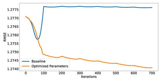
Figure 1.
A comparison of the convergence of the baseline MF algorithm on the CoMoDa dataset using the original parameters from [17] (blue) and GE optimized parameters (orange).
Although a 0.41% decrease in RMSE does not seem to be a very significant improvement, we should note that the GE enhanced MF algorithm achieved this level of performance without any manual tuning beyond the initial grammar settings. Compared to the amount of time we had to spend during our previous work for manual determination of the appropriate parameter values, this represents a significant reduction in the time which a practitioner has to spend tinkering with settings to obtain the first results. One should also note that an evaluation of 150 generations takes less time than setting parameter ranges manually.
5.2. Evolving New Latent Factors Update Equations
After a successful application of GE to a simple real parameter optimization, we now wanted to evolve a complete replacement for Equations (6) and (7). For that purpose, we used the following start symbol for the grammar:
= < expr >
= < expr >
Using this symbol, we can either evolve a complex equation (as seen in most of the item latent factor equations in Table 8) or a simple constant value. Note that during the evolution, we still used the values from Table 1 for evaluation of each single program in the population.
Table 8.
Best programs obtained from 10 evolution runs of 150 generations on the CoMoDa dataset.
This time, we let the evolution run for 150 generations, using the CoMoDa dataset again. Table 8 shows the ten best resulting equations for user and item latent factor calculation in addition to their RMSE score. Note that the actual equations produced by the evolution were quite hieroglyphic and the versions shown are mathematically equivalent equations simplified by hand. All 10 produced equations performed not only better than the hand-optimized baseline algorithm but also better than the GE optimized baseline version from the first part of the experiment. Compared to the average value of that we were able to achieve using only a parameter optimization, we now obtained an average RMSE value of with a standard deviation of . It was to be expected that the dispersion would now be greater as GE was given more freedom as to how to build the latent factors update expressions. A p-value of signifies that the results are significantly better than those obtained from the optimized baseline RMSE in the first part of the experiment. What is even more important, this time, we managed to obtain a program (i.e., the best program in Table 8) whose performance is more than 10% better than that of a baseline algorithm.
It is quite interesting to compare the evolved equations from Table 8 with those of the original algorithm (i.e., Equations (6) and (7)). We noticed that the evolved equations fixated latent factor values of a user. There seems to be one exception (i.e., the fifth row of the table), but as the equation simply copies a factor value to the next iteration, this value retains its initial value and can therefore be considered constant as well. The right column of Table 8 contains equations for calculating latent factor values of an item. After a closer inspection of the equations, we can observe that they are all very similar to Equation (7), only with quite a large learning rate and very small or even zero normalization constant . For example, in the first row of the table, we have and , and in the last row, we have and . In more than half of the equations, there is an additional constant factor whose interpretation is somehow ambiguous; it could be a kind of combination of a static bias and regularization. In summary, it is clear that GE diminished or sometimes even removed the regularization factor and greatly increased the learning rate in order to achieve the best possible result. Apart from that, it assigned the same constant value to all user latent factors. This could in turn signify that we are starting to experience the so-called bias-variance trade-off [59], where static biases take over a major part of contribution to variations in rating values.
5.3. Convergence Analysis
We have so far succeeded to evolve MF update equations that produced significantly better RMSE values than the original hand-optimized algorithm. During the second part of our experiment, we observed a notable increase in learning rate which made us believe that we do not actually need 100 iterations to reach the final values for the user and item factors. We generated the plot of the RMSE value as a function of iteration number to observe how the algorithm converges toward the final values.
The blue line in Figure 1 shows how the RMSE value changed during a run of a baseline MF algorithm using the original parameter values from Table 1, and the orange line shows the algorithm convergence using the optimized parameter values from the first row of Table 7. The noticeable jumps in the curves that happen every 100 iterations are a consequence of adding an additional latent factor into the calculation every 100 iterations as shown in the baseline algorithm.
We can observe that the unoptimized algorithm results in quite curious behavior. The smallest RMSE value is reached after only 65 iterations, but then it rapidly increases to a value even greater than the initial guess. The RMSE value stays larger than the initial one, even after adding additional factors and letting the MF algorithm run for 100 iterations for each one of the added factors. Conversely, using the GE optimized version of the MF algorithm, we obtain a curve whose RMSE score fell steadily toward the final, much better RMSE score.
Figure 2 shows how the RMSE value converges when we used the following equations as the update equations:
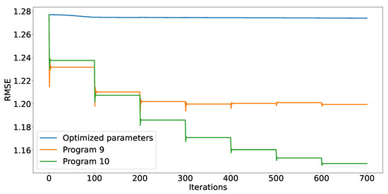
The equations are taken from the last and fourth row of Table 8, respectively. The most obvious difference from Figure 1 is a much more rapid convergence, which was to be expected as the learning rates are several orders of magnitude larger (this can be seen by rewriting Equations (10) and (9) back into the forms of (6) and (7), respectively). It seems that a learning rate of 40 and a regularization factor of (Equation (10)) are quite appropriate values as seen in Figure 2. However, the figure also shows how a learning rate of 140 (Equation (9)) already causes overshoots. At the same time, it seems that an absence of regularization produces overfitting which manifests itself as an increase in the RMSE values when the last two latent factors are added.
Either way, the algorithm converged in just a few iterations each time a new latent factor was added, indicating that much less than 100 iterations are actually needed. Thus, we reran all of the evolved programs on the same dataset, this time only using 20 iterations for each of the latent factors. We obtained exactly the same RMSE scores as we did with 100 iterations, which means that the calculation is now at least five times faster. This speedup is very important, especially when dealing with huge datasets that usually reside behind recommender systems. The results obtained by (9) and (10) using only 20 iterations are shown in Figure 3.
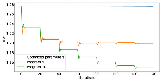
Figure 3.
Convergence of the RMSE value using the same equations as in Figure 2 but only 20 iterations.
5.4. MovieLens Dataset
In the next experiment, we wanted to evolve the update equations using a much larger dataset. We selected the MovieLens 100k dataset for the task while using the same starting symbol as in Section 5.2.
Because we switched to a different dataset, we first had to rerun our original baseline algorithm in order to obtain a new baseline RMSE, which now has a value of . Then, we ran over 20 evolutions, each of 150 generations. Table 9 shows the five best (and unique, as some RMSE values were repeated over several runs) evolved equations and their corresponding RMSE values. In summary, we achieved an average RMSE value of and a standard deviation of (with a minimum value of and a maximum value of ). We again used the Wilcoxon ranked sum test to confirm (with a p-value of ) that our numbers significantly differ from the baseline value.
Table 9.
MovieLens optimization results.
The most striking difference from the previous experiment is the fact that now all but one of the latent factors are in fact constants. Note that the third item latent factor in Table 9 is actually a constant because is a constant. This is a sign that a bias-variance trade-off as described in [59] has occurred. Because the MovieLens dataset contains a lot more ratings than the CoMoDa dataset, the information contained in the static biases becomes more prominent. This in turn means that there is almost no reason to calculate the remaining variance, which was automatically detected by GE. Using fixed latent factors also means that the algorithm can be completed within a single iteration, which is a huge improvement in the case of a very large dataset. More likely, the occurrence of constant factors will be used as a detection of over-saturation—when the equations produced by GE become constants, the operator knows that they must either introduce a time-dependent calculation of biases [19] or otherwise modify the algorithm (e.g., introduce new biases [17]).
5.5. Book-Crossing Dataset
In this experiment, we used the Book-Crossing dataset which is larger than the MovieLens dataset by a factor of 10. In addition, it features a different range of ratings (from 1 to 10 instead of 1 to 5) and covers a different type of item, namely books. Again, we first calculated the baseline RMSE which was now . We ran 20 evolutions of 150 generations each. Table 10 shows the five best evolved equations and their corresponding RMSE values. In summary, we achieved an average RMSE value of and a standard deviation of (with a minimum value of and a maximum value of ). We again used the Wilcoxon ranked sum test to confirm (with a p-value of ) that our numbers significantly differ from the baseline value.
Table 10.
Book-Crossing optimization results.
By observing the results, we can see a similar pattern as in the previous experiment—where one set of latent factors () is set to a static value, while the other changes its value during each iteration according to the current error value of . Because the dataset bears some similarities to the previous (MovieLens) in terms of saturation and ratios (ratings per user and per items), this was somehow expected.
5.6. Jester Dataset
In the last experiment, we used the Jester dataset. Again, we first calculated the baseline RMSE which was now . One should note that the number differs from those presented in Table 3 due to the fact that both cited articles ([41,44]) used a slightly different version of the dataset (either an expanded version or a filtered version). Although this means that we cannot directly compare our results, we can still see that we are in the same value range.
We ran 20 evolutions of 150 generations each. Table 11 shows the five best evolved equations and their corresponding RMSE values. In summary, we achieved an average RMSE value of and a standard deviation of (with a minimum value of and a maximum value of ). We again used the Wilcoxon ranked sum test to confirm (with a p-value of ) that our numbers significantly differ from the baseline value.
Table 11.
Jester optimization results.
Observing this last set of results, we find some similarities with the previous two experiments. One set of latent factors is again set to a static value. An interesting twist, however, is the fact that in this experiment the static value is assigned to the item latent factors () instead of the user latent factors. Upon reviewing the dataset characteristics, we can see that this further confirms the bias-variance trade-off. This is due to the fact that in this dataset the ratio of ratings per item is a hundred times larger than the ratio of ratings per user. The item’s biases therefore carry a lot more weight and thus reduce the importance of its latent factors. Once again, the GE approach detected this and adjusted the equations accordingly.
5.7. Result Summary
Table 12 shows a condensed version of our results. It can be seen that we managed to match or improve the performance of the MF algorithm on all four datasets. All the results were also tested using the Wilcoxon rank-sum test and, for each case, the test statistic was lower than the selected significance value of which confirms that our results were significantly different (better) than those of the baseline approach.
Table 12.
Result summary.
6. Conclusions
We used GE to successfully optimize the latent factors update equations of the MF algorithm on four diverse datasets. The approach works in an autonomous way which requires only the information about the range of ratings (e.g., 1 to 5, −10 to 10, etc.) and no additional domain knowledge. Such an approach is therefore friendly to any non-expert user who wants to use the MF algorithm on their database and does not have the knowledge and resources for a lengthy optimization study.
In the first part of the research, we limited the optimization process only to the parameter values, which already produced statistically significantly better RMSE values using 10-fold validation. After using the GE’s full potential to produce latent factor update equations, we observed an even better increase in the algorithm’s accuracy. Apart from even better RMSE values, this modification accelerated the basic MF algorithm for more than five times.
We then switched to three larger datasets that contained different item types and repeated our experiments. The results showed that GE almost exclusively assigned constant values to either user or item latent factors. It is outstanding how GE is able to gradually change—depending on the dataset size—the nature of the update equations from the classical stochastic gradient descent form, through a modified form where user latent factors are constants, to a form where both latent factors are constants. This way, GE adapts to the degree of a bias-variance trade-off present in a dataset and is able to dynamically warn about over-saturation.
A great potential of the usage of GE to support a MF-factorization-based recommender system lies in the fact that GE can be used as a black box to aid or even replace an administrator in initial as well as on-the-fly adjustments of a recommender system. Apart from that, GE can be used to generate warnings when the system becomes over-saturated and requires an administrator’s intervention. We believe that our results make a valuable contribution to the emerging field of employing evolutionary computing techniques in the development of recommender systems [26].
The presented approach therefore offers a nice quality-of-life upgrade to the existing MF algorithm but still has a few kinks that need to be ironed out. Although we are able to consistently optimize the algorithm and fit it to the selected dataset, the approach does require a lot of computational resources and time. This is not necessarily a drawback because we do not require real-time optimization but only need to run the algorithm once in a while to find the optimal settings.
For our future applications, we therefore plan to improve the algorithm’s performance by introducing parallel processing and to export parts of the code to C using the Cython library. In addition, we will also experiment with expanding the scope of our algorithm to optimizing the MF algorithm parameters as well (the number of iterations and latent factor, for example). We believe that this could lead to further improvements and potentially even speed up the MF method itself (by realizing that we need fewer iterations/factors, for example). It would also be interesting to test if we can apply our algorithm to other versions of the MF algorithm (graph-based, non-negative, etc.) and if we can apply our strategy to a completely different recommender system as well.
Author Contributions
Conceptualization, I.F.; Methodology, M.K. and Á.B.; Software, M.K.; Supervision, Á.B.; Writing—original draft, M.K.; Writing—review & editing, I.F. All authors have read and agreed to the published version of the manuscript.
Funding
This research received no external funding.
Institutional Review Board Statement
Not applicable.
Informed Consent Statement
Not applicable.
Data Availability Statement
Not applicable.
Acknowledgments
The authors acknowledge the financial support from the Slovenian Research Agency (research core funding No. P2-0246 ICT4QoL—Information and Communications Technologies for Quality of Life).
Conflicts of Interest
The authors declare no conflict of interest.
References
- Ahanger, G.; Little, T.D.C. Data semantics for improving retrieval performance of digital news video systems. IEEE Trans. Knowl. Data Eng. 2001, 13, 352–360. [Google Scholar] [CrossRef]
- Uchyigit, G.; Clark, K. An Agent Based Electronic Program Guide. In Proceedings of the 2nd Workshop on Personalization in Future TV, Malaga, Spain, 28 May 2002; pp. 52–61. [Google Scholar]
- Kurapati, K.; Gutta, S.; Schaffer, D.; Martino, J.; Zimmerman, J. A multi-agent TV recommender. In Proceedings of the UM 2001 workshop Personalization in Future TV, Sonthofen, Germany, 13–17 July 2001. [Google Scholar]
- Bezerra, B.; de Carvalho, F.; Ramalho, G.; Zucker, J. Speeding up recommender systems with meta-prototypes. In Brazilian Symposium on Artificial Intelligence; Springer: Berlin/Heidelberg, Germany, 2002; pp. 521–528. [Google Scholar]
- Yuan, J.L.; Yu, Y.; Xiao, X.; Li, X.Y. SVM Based Classification Mapping for User Navigation. Int. J. Distrib. Sens. Netw. 2009, 5, 32. [Google Scholar] [CrossRef]
- Pogačnik, M. Uporabniku Prilagojeno Iskanje Multimedijskih Vsebin. Ph.D. Thesis, University of Ljubljana, Ljubljana, Slovenia, 2004. [Google Scholar]
- Hand, D.J.; Mannila, H.; Smyth, P. Principles of Data Mining; MIT Press: Cambridge, MA, USA, 2001. [Google Scholar]
- Salton, G.; McGill, M.J. Introduction to Modern Information Retrieval; McGraw-Hill, Inc.: New York, NY, USA, 1986. [Google Scholar]
- Barry Crabtree, I.; Soltysiak, S.J. Identifying and tracking changing interests. Int. J. Digit. Libr. 1998, 2, 38–53. [Google Scholar] [CrossRef]
- Mirkovic, J.; Cvetkovic, D.; Tomca, N.; Cveticanin, S.; Slijepcevic, S.; Obradovic, V.; Mrkic, M.; Cakulev, I.; Kraus, L.; Milutinovic, V. Genetic Algorithms for Intelligent Internet search: A Survey and a Package for Experimenting with Various Locality Types. IEEE TCCA Newsl. 1999, pp. 118–119. Available online: https://scholar.google.co.jp/scholar?q=Genetic+algorithms+for+intelligent+internet+search:+A+survey+and+a+++package+for+experimenting+with+various+locality+types&hl=zh-CN&as_sdt=0&as_vis=1&oi=scholart (accessed on 1 February 2022).
- Mladenic, D. Text-learning and related intelligent agents: A survey. IEEE Intell. Syst. 1999, 14, 44–54. [Google Scholar] [CrossRef]
- Malone, T.; Grant, K.; Turbak, F.; Brobst, S.; Cohen, M. Intelligent Information Sharing Systems. Commun. ACM 1987, 30, 390–402. [Google Scholar] [CrossRef]
- Buczak, A.L.; Zimmerman, J.; Kurapati, K. Personalization: Improving Ease-of-Use, trust and Accuracy of a TV Show Recommender. In Proceedings of the 2nd Workshop on Personalization in Future TV, Malaga, Spain, 28 May 2002. [Google Scholar]
- Difino, A.; Negro, B.; Chiarotto, A. A Multi-Agent System for a Personalized Electronic Programme Guide. In Proceedings of the 2nd Workshop on Personalization in Future TV, Malaga, Spain, 28 May 2002. [Google Scholar]
- Guna, J.; Stojmenova, E.; Kos, A.; Pogačnik, M. The TV-WEB project—Combining internet and television—Lessons learnt from the user experience studies. Multimed. Tools Appl. 2017, 76, 20377–20408. [Google Scholar] [CrossRef]
- Kunaver, M.; Požrl, T. Diversity in Recommender Systems A Survey. Knowl. Based Syst. 2017, 123, 154–162. [Google Scholar] [CrossRef]
- Odic, A.; Tkalcic, M.; Tasic, J.F.; Kosir, A. Predicting and Detecting the Relevant Contextual Information in a Movie-Recommender System. Interact. Comput. 2013, 25, 74–90. [Google Scholar] [CrossRef][Green Version]
- Rodriguez, M.; Posse, C.; Zhang, E. Multiple Objective Optimization in Recommender Systems. In Proceedings of the Sixth ACM Conference on Recommender Systems, RecSys’12, Dublin, Ireland, 9–13 September 2021; ACM: New York, NY, USA, 2012; pp. 11–18. [Google Scholar] [CrossRef]
- Koren, Y. Collaborative Filtering with Temporal Dynamics. Commun. ACM 2010, 53, 89–97. [Google Scholar] [CrossRef]
- Koren, Y.; Bell, R.; Volinsky, C. Matrix Factorization Techniques for Recommender Systems. Computer 2009, 42, 30–37. [Google Scholar] [CrossRef]
- Hug, N. Surprise, a Python Library for Recommender Systems. 2017. Available online: http://surpriselib.com (accessed on 1 March 2022).
- Pedregosa, F.; Varoquaux, G.; Gramfort, A.; Michel, V.; Thirion, B.; Grisel, O.; Blondel, M.; Prettenhofer, P.; Weiss, R.; Dubourg, V.; et al. Scikit-learn: Machine Learning in Python. J. Mach. Learn. Res. 2011, 12, 2825–2830. [Google Scholar]
- Mnih, A.; Salakhutdinov, R.R. Probabilistic matrix factorization. In Advances in Neural Information Processing Systems; The MIT Press: Cambridge, MA, USA, 2008; pp. 1257–1264. [Google Scholar]
- Rosenthal, E. Explicit Matrix Factorization: ALS, SGD, and All That Jazz. 2017. Available online: https://blog.insightdatascience.com/explicit-matrix-factorization-als-sgd-and-all-that-jazz-b00e4d9b21ea (accessed on 19 March 2018).
- Yu, H.F.; Hsieh, C.J.; Si, S.; Dhillon, I.S. Parallel matrix factorization for recommender systems. Knowl. Inf. Syst. 2014, 41, 793–819. [Google Scholar] [CrossRef]
- Horváth, T.; Carvalho, A.C. Evolutionary Computing in Recommender Systems: A Review of Recent Research. Nat. Comput. 2017, 16, 441–462. [Google Scholar] [CrossRef]
- Salehi, M.; Kmalabadi, I.N. A Hybrid Attribute-based Recommender System for E-learning Material Recommendation. IERI Procedia 2012, 2, 565–570. [Google Scholar] [CrossRef][Green Version]
- Zandi Navgaran, D.; Moradi, P.; Akhlaghian, F. Evolutionary based matrix factorization method for collaborative filtering systems. In Proceedings of the 2013 21st Iranian Conference on Electrical Engineering (ICEE), Mashhad, Iran, 14–16 May 2013; pp. 1–5. [Google Scholar]
- Hu, L.; Cao, J.; Xu, G.; Cao, L.; Gu, Z.; Zhu, C. Personalized Recommendation via Cross-domain Triadic Factorization. In Proceedings of the 22nd International Conference on World Wide Web, WWW’13, Rio de Janeiro, Brazil, 13–17 May 2013; ACM: New York, NY, USA, 2013; pp. 595–606. [Google Scholar] [CrossRef]
- Balcar, S. Preference Learning by Matrix Factorization on Island Models. In Proceedings of the 18th Conference Information Technologies—Applications and Theory (ITAT 2018), Hotel Plejsy, Slovakia, 21–25 September 2018; Volume 2203, pp. 146–151. [Google Scholar]
- Rezaei, M.; Boostani, R. Using the genetic algorithm to enhance nonnegative matrix factorization initialization. Expert Syst. 2014, 31, 213–219. [Google Scholar] [CrossRef]
- Lara-Cabrera, R.; Gonzalez-Prieto, Á.; Ortega, F.; Bobadilla, J. Evolving Matrix-Factorization-Based Collaborative Filtering Using Genetic Programming. Appl. Sci. 2020, 10, 675. [Google Scholar] [CrossRef]
- O’Neil, M.; Ryan, C. Grammatical Evolution. In Grammatical Evolution: Evolutionary Automatic Programming in an Arbitrary Language; Springer: Boston, MA, USA, 2003; pp. 33–47. [Google Scholar] [CrossRef]
- Bokde, D.K.; Girase, S.; Mukhopadhyay, D. An Approach to a University Recommendation by Multi-criteria Collaborative Filtering and Dimensionality Reduction Techniques. In Proceedings of the 2015 IEEE International Symposium on Nanoelectronic and Information Systems, Indore, India, 21–23 December 2015; pp. 231–236. [Google Scholar] [CrossRef]
- Košir, A.; Odić, A.; Kunaver, M.; Tkalčič, M.; Tasič, J.F. Database for contextual personalization. Elektroteh. Vestn. 2011, 78, 270–274. [Google Scholar]
- Breese, J.S.; Heckerman, D.; Kadie, C. Empirical analysis of predictive algorithms for collaborative filtering. In Proceedings of the Fourteenth Conference on Uncertainty in Artificial Intelligence, Madison Wisconsin, 24–26 July 1998; Morgan Kaufmann Publishers Inc.: Burlington, MA, USA, 1998; pp. 43–52. [Google Scholar]
- Herlocker, J.L.; Konstan, J.A.; Borchers, A.; Riedl, J. An Algorithmic Framework for Performing Collaborative Filtering. In Proceedings of the 22nd Annual International ACM SIGIR Conference on Research and Development in Information Retrieval, SIGIR’99, Berkeley, CA, USA, 15–19 August 1999; ACM: New York, NY, USA, 1999; pp. 230–237. [Google Scholar] [CrossRef]
- Shardanand, U.; Maes, P. Social information filtering: Algorithms for automating ‘word of mouth’. In Proceedings of the SIGCHI Conference on Human Factors in Computing Systems, Denver, CO, USA, 7–11 May 1995; ACM Press/Addison-Wesley Publishing Co., Ltd.: Boston, MA, USA, 1995; pp. 210–217. [Google Scholar]
- Bao, Z.; Xia, H. Movie Rating Estimation and Recommendation, CS229 Project; Stanford University: Stanford, CA, USA, 2012; pp. 1–4. [Google Scholar]
- Chandrashekhar, H.; Bhasker, B. Personalized recommender system using entropy based collaborative filtering technique. J. Electron. Commer. Res. 2011, 12, 214. [Google Scholar]
- Ranjbar, M.; Moradi, P.; Azami, M.; Jalili, M. An imputation-based matrix factorization method for improving accuracy of collaborative filtering systems. Eng. Appl. Artif. Intell. 2015, 46, 58–66. [Google Scholar] [CrossRef]
- Kunaver, M.; Fajfar, I. Grammatical Evolution in a Matrix Factorization Recommender System. In Proceedings of the International Conference on Artificial Intelligence and Soft Computing, Zakopane, Poland, 12–16 June 2016; Rutkowski, L., Korytkowski, M., Scherer, R., Tadeusiewicz, R., Zadeh, L.A., Zurada, J.M., Eds.; Springer: Berlin/Heidelberg, Germany, 2016; Volume 9692, pp. 392–400. [Google Scholar] [CrossRef]
- Chen, H.H. Weighted-SVD: Matrix Factorization with Weights on the Latent Factors. arXiv 2017, arXiv:1710.00482. [Google Scholar]
- Yu, T.; Mengshoel, O.J.; Jude, A.; Feller, E.; Forgeat, J.; Radia, N. Incremental learning for matrix factorization in recommender systems. In Proceedings of the 2016 IEEE International Conference on Big Data (Big Data), Washington, DC, USA, 5–8 December 2016; pp. 1056–1063. [Google Scholar]
- Tashkandi, A.; Wiese, L.; Baum, M. Comparative Evaluation for Recommender Systems for Book Recommendations. In BTW (Workshops); Mitschang, B., Ritter, N., Schwarz, H., Klettke, M., Thor, A., Kopp, O., Wieland, M., Eds.; Hair Styling & Makeup Servi: Hong Kong, China, 2017; Volume P-266, pp. 291–300. Available online: https://www.broadwayteachinggroup.com/about-btw (accessed on 1 February 2021).
- Ryan, C.; Azad, R.M.A. Sensible Initialisation in Chorus. In Proceedings of the European Conference on Genetic Programming, Essex, UK, 14–16 April 2003; Ryan, C., Soule, T., Keijzer, M., Tsang, E.P.K., Poli, R., Costa, E., Eds.; Springer: Berlin/Heidelberg, Germany, 2003; Volume 2610, pp. 394–403. [Google Scholar] [CrossRef]
- Koza, J. Genetic Programming: On the Programming of Computers by Means of Natural Selection; The MIT Press: Cambridge, MA, USA, 1992. [Google Scholar]
- Kunaver, M.; Žic, M.; Fajfar, I.; Tuma, T.; Bűrmen, Á.; Subotić, V.; Rojec, Ž. Synthesizing Electrically Equivalent Circuits for Use in Electrochemical Impedance Spectroscopy through Grammatical Evolution. Processes 2021, 9, 1859. [Google Scholar] [CrossRef]
- Kunaver, M. Grammatical evolution-based analog circuit synthesis. Inf. MIDEM 2019, 49, 229–240. [Google Scholar]
- Poikolainen, I.; Neri, F.; Caraffini, F. Cluster-Based Population Initialization for differential evolution frameworks. Inf. Sci. 2015, 297, 216–235. [Google Scholar] [CrossRef]
- Harper, R.; Blair, A. A Structure Preserving Crossover In Grammatical Evolution. In Proceedings of the 2005 IEEE Congress on Evolutionary Computation, Edinburgh, UK, 2–5 September 2005; Volume 3, pp. 2537–2544. [Google Scholar]
- Byrne, J.; O’Neill, M.; Brabazon, A. Structural and Nodal Mutation in Grammatical Evolution. In Proceedings of the 11th Annual Conference on Genetic and Evolutionary Computation, GECCO’09, Montreal, QC, Canada, 8–12 July 2009; ACM: New York, NY, USA, 2009; pp. 1881–1882. [Google Scholar] [CrossRef]
- Helmuth, T.; Spector, L.; Martin, B. Size-based Tournaments for Node Selection. In Proceedings of the 13th Annual Conference Companion on Genetic and Evolutionary Computation GECCO’11, Dublin, Ireland, 12–16 July 2011; pp. 799–802. [Google Scholar]
- Luke, S.; Panait, L. A Comparison of Bloat Control Methods for Genetic Programming. Evol. Comput. 2006, 14, 309–344. [Google Scholar] [CrossRef]
- Poli, R.; Langdon, W.; McPhee, N. A Field Guide to Genetic Programming; Lulu Enterprises UK Ltd.: Cardiff, Glamorgan, UK, 2008. [Google Scholar]
- GroupLens. MovieLens. 2017. Available online: https://grouplens.org/blog/2017/07/ (accessed on 19 March 2018).
- Ziegler, C.N.; McNee, S.M.; Konstan, J.A.; Lausen, G. Improving recommendation lists through topic diversification. In Proceedings of the 14th International Conference on World Wide Web (WWW), Seoul, Korea, 7–11 April 2005. [Google Scholar]
- Goldberg, K.; Roeder, T.; Gupta, D.; Perkins, C. Eigentaste: A Constant Time Collaborative Filtering Algorithm. Inf. Retr. 2001, 4, 133–151. [Google Scholar] [CrossRef]
- Aggarwal, C.C. Recommender Systems—The Textbook; Springer: Berlin/Heidelberg, Germany, 2016; pp. 1–498. [Google Scholar]
Publisher’s Note: MDPI stays neutral with regard to jurisdictional claims in published maps and institutional affiliations. |
© 2022 by the authors. Licensee MDPI, Basel, Switzerland. This article is an open access article distributed under the terms and conditions of the Creative Commons Attribution (CC BY) license (https://creativecommons.org/licenses/by/4.0/).