Out of the Niche: Using Direct Search Methods to Find Multiple Global Optima

Abstract

Multimodal optimization deals with problems where multiple feasible global solutions coexist. Despite sharing a common objective function value, some global optima may be preferred to others for various reasons. In such cases, it is paramount to devise methods that are able to find as many global optima as possible within an affordable computational budget. Niching strategies have received an overwhelming attention in recent years as the most suitable technique to tackle these kinds of problems. In this paper we explore a different approach, based on a systematic yet versatile use of traditional direct search methods. When tested over reference benchmark functions, our proposal, despite its apparent simplicity, noticeably resists the comparison with state-of-the-art niching methods in most cases, both in the number of global optima found and in the number of function evaluations required. However, rather than trying to outperform niching methods—far more elaborated—our aim is to enrich them with the knowledge gained from exploiting the distinctive features of direct search methods. To that end, we propose two new performance measures that can be used to evaluate, compare and monitor the progress of optimization algorithms of (possibly) very different nature in their effort to find as many global optima of a given multimodal objective function as possible. We believe that adopting these metrics as reference criteria could lead to more sophisticated and computationally-efficient algorithms, which could benefit from the brute force of derivative-free local search methods.

1. Introduction

Generally speaking, optimization aims at finding local or global solutions of a given problem, commonly expressed by means of an objective function and, possibly, several constraints. Depending on the characteristics of the objective function, the constraints, the search space and various other considerations, a plethora of optimization techniques have been devised in the last decades.

In this paper, we focus on bound-constrained optimization problems of the form

$$\underset{x\in \mathcal{S}\subset {\mathbb{R}}^n}{max}f\left(x\right),$$

(1)

where $f\left(x\right)$ is assumed to be multimodal, i.e., it has more than one global solution. The n-dimensional search space $\mathcal{S}$ is defined as $l_i\le x_i\le u_i,i=1,\dots ,n$, where $l_i$’s and $u_i$’s are, respectively, the lower and upper bounds for the i-th dimension. For convenience, we deal with maximization problems in what follows, although our methodology can be easily adapted to minimization problems.

Multimodal optimization (MMO) aims to locate as many global optima of the objective function as possible. Such problem has been the subject of intensive study in recent years, giving rise to valuable advances in solution methods [1]. Finding multiple global optima is usually a hard task, especially as the problem dimension grows. In return, knowledge of different optimal alternatives can be of great interest in many areas, like engineering, finances or science, where some solutions—despite resulting in the same optimal system performance—may be favored against others due to e.g., physical, cost or robustness reasons, see [2,3]. Multiple solutions could also be analyzed to discover hidden properties or relationships of the underlying optimization problem, allowing to acquire domain knowledge [4].

Various methods have been contrived in recent years to efficiently tackle the problem of finding multiple global optima in continuous optimization [5]. Most of the proposed routines fall under the broad umbrella of Evolutionary Algorithms (EAs), a class of methods which maintain a population of possible solutions, changing it after every generation according to certain rules [6]. EAs encompass various subfamilies, being Genetic Algorithms (GAs) [7], Evolution Strategy (ES) [8], Differential Evolution (DE) [9] and Particle Swarm Optimization (PSO) [10] the most popular ones. Very little work, in contrast, has been devoted to solving the multimodal problem (1) using non-EA-related techniques. For instance, in a seminal paper [11] proposed a versatile and practical method of searching the parameter space. That gave rise to the so-called Bayesian global optimization, where stochastic processes are used to develop figures of merit for where to take search points, balancing local and global search in an attractive fashion, see [12] for further insight. In another remarkable work, Ref. [13] introduced a response surface methodology to model nonlinear, multimodal functions and showed how to build an efficient global optimization algorithm based on these approximating functions.

Intimately related to EAs, niching refers to the technique of finding and preserving multiple stable niches—defined as favorable parts of the solution space, possibly around multiple solutions—so that convergence to a single solution is prevented, see [14,15]. Niching strategies have been implemented, in some way or another, within all the variants of the EA algorithms mentioned above to solve MMO problems. To wit, a niching framework utilizing derandomized ES was introduced by [16], proposing the CMA-ES as a niching optimizer for the first time. An approach that does not use any radius to separate the population into subpopulations (or species) but employs the space topology instead, was proposed in [17]. These GA/ES-flavored niching methods have successfully been adapted to the DE methodology to solve MMO problems, see [18] for a comprehensive treatment. Finally, Ref. [19] presents a thorough review of PSO-based algorithms designed to find multiple global optima.

As an attempt to enhance GAs by taking advantage of the local properties of the objective function, memetic algorithms—or hybrid genetic algorithms, as they are also sometimes referred to, see [7]—are, in essence, GAs coupled with a suitable local search heuristic [20]. They have been explored as an alternative methodology to solve MMO problems with promising results [21,22].

Taking that strategy to the extreme, we propose here a novel approach to solve MMO problems, in which we rely exclusively on local direct search methods, suitably implementing them in a flexible yet rigorous manner. To the best of our knowledge, this is the first attempt to deal with these kinds of problems in such way. It is important to emphasize that our proposal does not make use of evolutionary algorithms but, rather, it relies exclusively on direct search methods as the only methodological tool to try to find as many global optima as possible. Aiming to contextualize the performance of our methods when compared to evolutionary algorithms, we used two baseline niching algorithms as a reference. Far from being an exotic, barely efficient, alternative, our methodology compares nicely with cutting-edge niching methods when tested over a set of reference benchmark functions, as we will discuss later on. Furthermore, carefully tracking down the iterates obtained when applying direct search methods allows us to define two new dynamic performance measures: the moving peak ratio—represented by the so-called performance curve—and the moving success rate. These new metrics—together with the knowledge gathered by comparing the performance of different direct search methods—could be used to hint at potential ways of improvement of the far more convoluted evolutionary algorithms.

The rest of the paper is organized as follows. In Section 2, we present a review of classical direct search methods in the context of bound-constrained global optimization. Section 3 briefly describes the benchmark functions used to test our methods. In turn, Section 4 deals with specific implementation details of our strategy, whereas in Section 5, we analyze the numerical results obtained. We end with some discussion.

2. Direct Search Methods

The problem of finding global/local optima of a bound-constrained multimodal function with local search methods has traditionally been addressed from two different perspectives: (1) using methods which compute function derivatives; or (2) implementing derivative-free methods. Although the superiority of the former is now undisputed (when applicable), these Newton-based methods require the use of, at least, first- and, possibly, second-order information to compute a “good” search direction and a steplength, which will eventually allow them to converge to a local optimum. However, there are situations where these methods might actually fail to work, including when: (i) the evaluation of the objective function is inaccurate; (ii) the objective function is not smooth; and/or (iii) its derivatives are unavailable or unreliable.

Derivative-free methods are a suitable alternative to circumvent these drawbacks, since they do not compute derivatives of the objective function explicitly. This family of methods is usually further divided into two broad categories: (1) Methods that approximate derivatives by constructing a model of the objective function [23]. This approach is not well suited to deal with simulation-based optimization, nonnumerical functions, or non-smooth or discontinuous functions. (2) Direct search methods [24], which stand as the best alternative to seek for local or global optima when derivatives can be neither computed nor approximated.

We aim at solving convoluted MMO problems with the only aid of direct search methods. These methods are usually organized into three basic groups [25]: (1) pattern search, (2) simplex search, and (3) methods with adaptive sets of directions. In what follows, we review their main features, laying special emphasis on the most popular representatives within each category.

2.1. Pattern Search Methods

These methods are characterized by a set of exploratory moves, which only consider the value of the objective function [26]. Such moves lie, in general, on an n-dimensional rational lattice and consist of a systematic strategy for visiting the incumbent lattice points. Although a search pattern requires at least $n+1$ points per iteration, a single iteration may spend as few as one function evaluation (FE) because the search needs only simple improvement of the objective function to accept a new point. Additionally, the lengths of trial steps may change between iterations, but the relative location of the trial points must maintain a particular structure.

An iteration of a pattern search algorithm compares the value of the objective function at the current iterate and (at least) some subset of points in the pattern. At each iteration either: (i) a trial point yields improvement and becomes the new iterate; or (ii) no increase in value is found at any point in the pattern. In the latter case, the scale factor of the lattice is reduced, and the next iteration continues the search on a finer grid. This process continues until some termination criterion is fulfilled.

There are several algorithms within this category, being three of the most widely-used ones the Compass Search (CS) [27], Hooke and Jeeves [24] and multidirectional search [28] methods. For brevity reasons, we only discuss briefly the first one, referring the reader to the bibliography for the other two methods.

Compass Search Method

CS makes exploratory moves from the current iterate to trial points obtained by moving a given steplenght up and down each coordinate direction. If the search finds simple improvement at any trial point, the exploratory move relocates there and a new iteration begins. Otherwise, the iteration is deemed unsuccessful, and the steplength is reduced to allow for a finer search. The procedure stops when the steplength falls below a predefined tolerance value.

2.2. Simplex Search Methods

This family of methods maintain a set of points, located at the vertices of an n-dimensional simplex. At each iteration, they attempt to replace the worst point by a new and better one using reflection, expansion, and/or contraction moves. Most methods within this category are, to a greater or lesser extent, variations of the pioneer Nelder-Mead method (NM) [29], which we review below (see [30] for a stochastic implementation for simulation optimization).

Nelder-Mead Method

A simplex is defined as the geometrical figure consisting of $n+1$ points (or vertices) and all their interconnecting line segments and polygonal faces. If any point of a nondegenerate simplex is taken as the origin, then the remaining points define vector directions spanning the whole search space.

Once started, the uphill simplex method takes a series of steps: (1) most are reflections, moving the simplex point with the lowest function value through the opposite simplex face to a new better point; (2) expansions, trying, when possible, to stretch out the simplex in one or another direction to take larger steps; (3) contractions, when the method gets trapped in a flat valley-shaped region and tries to contract itself in the transverse direction to escape; (4) sometimes, when trying to “pass through the eye of a needle”, the method would contract in all directions, pulling itself in around its best point [31].

2.3. Methods with Adaptive Sets of Search Directions

This family of methods perform the search by constructing directions designed to use information about the curvature of the objective obtained during the course of the search. Two of the most popular algorithms within this branch are Rosenbrock’s (RB) [32] and Powell’s search [33] methods, which we briefly review below.

2.3.1. Rosenbrock’s Method

Rosenbrock’s algorithm, together with the improvements made by Palmer, is an enhanced procedure for generating orthogonal search vectors to be used in Rosenbrock’s and Swann’s direct search optimization methods [32].

In such methods, local optima are sought by conducting univariate searches of different steplengths parallel to each of the orthogonal unit vectors in the search space, constituting one “stage” of the calculation. For the next stage, a new set of orthogonal unit vectors is generated, such that the first vector lies along the direction of greatest improvement on the previous phase.

2.3.2. Powell’s Search Method

In this method, each iteration begins with a search down n linearly independent directions starting from the best known approximation to the optimum. These directions are initially chosen as the coordinate axes, so the start of the first iteration is identical to an iteration of the CS method which changes one parameter at a time. This method is modified to generate conjugate directions by making each iteration define a new direction, and choosing the linearly independent directions for the next iterations accordingly. Some variations of this basic algorithm are discussed in [33].

3. Benchmark Functions for the Niching Competition

In testing the performance of direct search methods, we consider the set of problems defined in the 2013 Competition on Niching Methods for Multimodal Optimization [34]. Those benchmark functions have been used ever since as reference functions at various other genetic and evolutionary competitions. It is composed of 20 multimodal test functions formulated as optimization problems: (1) $F_1$: Five-Uneven-Peak Trap (1D); (2) $F_2$: Equal Maxima (1D); (3) $F_3$: Uneven Decreasing Maxima (1D); (4) $F_4$: Himmelblau (2D); (5) $F_5$: Six-Hump Camel Back (2D); (6) $F_6$: Shubert (2D, 3D); (7) $F_7$: Vincent (2D, 3D); (8) $F_8$: Modified Rastrigin—All Global Optima (2D); (9) $F_9$: Composition Function 1 (2D); (10) $F_{10}$: Composition Function 2 (2D); (11) $F_{11}$: Composition Function 3 (2D, 3D, 5D, 10D); (12) $F_{12}$: Composition Function 4 (3D, 5D, 10D, 20D).

For each test function, the following information is available, see [34] for the specific values for each function: (i) The number of known global optima NKP; (ii) The peak height ph, defined as the value of the objective function at the global optima; (iii) A niche radius r value that can sufficiently distinguish two closest global optima.

The competition was originally conceived to compare the capability of different niching algorithms to locate all global optima. To that aim, a level of accuracy $ϵ$ is defined as a threshold value for the objective value, under which it is considered that a global optima has been found. The competition establishes five different accuracy level s $ϵ=\{{10}^{-1},{10}^{-2},{10}^{-3},{10}^{-4},{10}^{-5}\}$.

A niching algorithm with arbitrary population size would try to solve every test function for each accuracy level, and it would then be determined how many global optima it has been able to find without exceeding a fixed maximum number of function evaluations MaxFEs, see [34] for details. The competition allows to execute $\mathtt{NR}=\mathtt{50}$ runs of the previous scheme. Each run is initialized using uniform random seeds within the search space.

The success of any competing algorithm is measured in terms of three key performance indicators:

• The peak ratio PR, defined as the average percentage of all known global optima found over the NR runs,

  $$\mathtt{PR}=\frac{{\sum }_{i=1}^{\mathtt{NR}}{\mathtt{NPF}}_i}{\mathtt{NKP}·\mathtt{NR}},$$

  (2)

  where ${\mathtt{NPF}}_i$ denotes the number of global optima found in the end of the i-th run.
• The success rate SR, computed as the percentage of successful runs, defined, in turn, as those runs where all known global optima are found,

  $$\mathtt{SR}=\frac{\mathtt{NSR}}{\mathtt{NR}},$$

  (3)

  where NSR denotes the number of successful runs.
• The average number of function evaluations AveFEs required to find all known global optima

  $$\mathtt{AveFEs}=\frac{{\sum }_{i=1}^{\mathtt{NR}}{\mathtt{FE}}_i}{\mathtt{NR}},$$

  (4)

  where ${\mathtt{FE}}_i$ denotes the number of evaluations used in the i-th run. This is a measure of the algorithm’s convergence speed. If the algorithm cannot locate all the global optima within the maximum allowed number of function evaluations in a particular run, then such run will contribute to the calculation of AveFEs with MaxFEs.

Once all these performance measures have been defined, niching algorithms are ranked according to their PR. In case of ties, the algorithm with the lower AveFEs is preferred, see [34] for details.

3.1. Nominating Direct Methods for the Competition

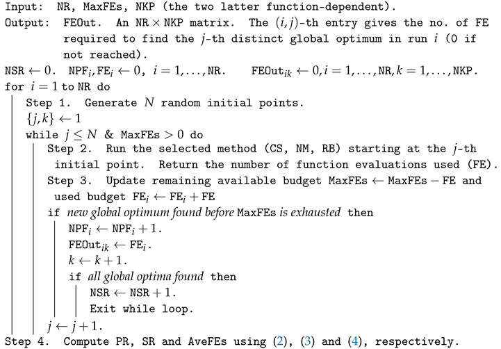
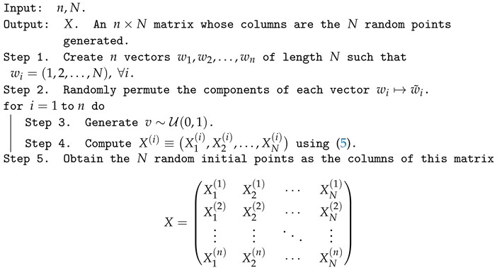
Direct search methods follow a distinctively different strategy than that of niching methods, as outlined in Algorithm 1. For each run, an arbitrary and sufficiently large number of initial points N is sampled from some suitable random-generating mechanism. This is the equivalent of the arbitrary initial population in genetic algorithms, and we choose it sufficiently large so we can guarantee that we will never run out of points before either finding all known global optima, or exhausting the FE budget. Then, each initial point is used as the seed of a given direct search method, which will find its way across the search space of the test function, according to the specific rules upon which such method is designed. If successful, the nominated direct search method may be able to find a global optimum within the allowed budget. Otherwise, by the time no more FEs are available, it might either still wander erratically around the intricacies of the objective function or be stuck on a local optimum, a saddle point, or any other type of undesired point.

Algorithm 1: Multimodal optimization strategy using Direct Search Methods.

The figure of interest for the current run is the number of distinct known global optima found within the total budget of function evaluations MaxFEs. Should all known global optima be located before such budget is depleted, we would stop the current run and start a new one, resetting the FE counter to zero. The above scheme would be replicated $\mathtt{NR}=\mathtt{50}$ times, after which we would then compute the three performance measures PR, SR and FE for the corresponding direct search method.

In order to gain further insight into the accomplishment of our methods, we have devised two new performance metrics. First, for a given run we are interested in knowing how many function evaluations were required on average to find the first global optimum of a given objective function, the first two global optima and so on. To do so, we define what we call the moving peak ratio mPR as the proportion of the total number of global optima found at the current stage of the optimization process on a given run. Therefore, mPR could theoretically take values $\{0,1/\mathrm{NKP},2/\mathrm{NKP},\dots ,1\}$ for a given test function with NKP known global optima, 0 meaning that no global optima has yet been reached and 1 that all have already been found. Note that the largest values of mPR might never be attained for some functions, indicating that the corresponding method was not able to find all known global optima. Then, for a given (attained) value of mPR, we record the average number of function evaluations AveFEs (computed over the NR runs) that was needed to find the corresponding number of global optima $\nu \left(\mathrm{mPR}\right)=\mathrm{mPR}·\mathrm{NKP}$ for a given accuracy level $ϵ$. By plotting all attained mPR vs AveFEs pairs, we obtain the so-called performance curve. Each point in the curve corresponds to the average number of function evaluations that was needed to find the number of global optima $\nu \left(\mathtt{mPR}\right)$ associated with the matching mPR.

The second metric is intended to assess the robustness of our methods. To that aim, we adapt (3) to define the moving success rate mSR as the proportion of runs that were actually able to find the number of global optima indicated by $\nu \left(\mathtt{mPR}\right)$, i.e.,

$$\mathtt{mSR}=\frac{\mathtt{NSR}\left(\nu \right(\mathtt{mPR}\left)\right)}{\mathtt{NR}},$$

where $\mathtt{NSR}\left(\nu \right(\mathtt{mPR}\left)\right)$ indicates the number of such successful runs.

To compute these novel performance measures, we must keep track of the number of function evaluations used by our methods each time they find a new global optimum in every run. Up to our knowledge, this is the first time that this exhaustive information is used in the way we propose. Therefore, when considering these innovative dynamic criteria, we will contrast our proposals with those niching methods participating in the most recent genetic and evolutionary competitions from a wider perspective. We believe a better understanding could emerge from such comparison, helping us detect potential weaknesses and strong points of either class of methods in their attempt to find all known global optima in a faster way.

4. Implementation

We discuss now several implementation considerations that are crucial for a good performance of the direct search methods used in our analysis.

4.1. Latin Hypercube Sampling

Like any other algorithm, direct search methods need initial points to start running. How these seeds are randomly generated is vital to the performance of the methods. The underlying idea is to sample the initial points in a “sufficiently and suitably dispersed” manner, so as to cover the search space in the most adequate possible way. Different near-random generating schemes are available in the literature [35], being the Latin Hypercube Sampling (LHS) [36,37] one of the most popular and versatile ones, and the one we have used in our computations.

The specific way in which we implement the LHS for an n-dimensional function is outlined in Algorithm 2. First, we create n vectors $w_1,w_2,\dots ,w_n$ with length equal to the initial population size N, which coincides with the number of divisions of the function domain along each dimension, effectively partitioning the sample space into $N^n$ identical hypercubes. The entries of each vector are initially labeled sequentially from 1 to N, and then randomly permuted. The rearranged vectors ${\tilde{w}}_1,{\tilde{w}}_2,\dots ,{\tilde{w}}_n$ contain the “coordinates” of the N hypercells randomly drawn from the pool of $N^n$ candidates. Each of these selected hypercubes constitutes the sampling space for exactly one of the N initial points, which will be randomly generated from a multidimensional uniform distribution. The N-dimensional vector $X^{\left(i\right)}$, containing the i-th coordinate of the N random points $X_1,X_2,\dots ,X_N$, would be then computed as

$$X^{\left(i\right)}\equiv \left(X_1^{\left(i\right)},X_2^{\left(i\right)},\dots ,X_N^{\left(i\right)}\right)=l_i+\frac{\left(u_i-l_i\right)}{N}(\upsilon +{\tilde{w}}_i-\mathbb{1}),i=1,\dots ,n,$$

(5)

where $l_i$ and $u_i$ are, respectively, the lower and upper bounds of the i-th dimension for the incumbent test function, $\upsilon$ is an N-vector of uniform random numbers $\mathcal{U}(0,1)$, and $𝟙$ is an N-vector of all ones.    

Algorithm 2: Latin Hypercube Sampling Algorithm.

As an illustration, let us consider the trivial case $n=2$ and $N=3$, where we would have $3^2=9$ “hypercubes” (squares in this case). The lower and upper bounds would be 2-dimensional vectors, $l=\left(l_1,l_2\right)$ and $u=\left(u_1,u_2\right)$. We would create two vectors, $w_1$ and $w_2$, and initialize them as $(1,2,3)$. After the permutation, one possible outcome could be e.g., ${\tilde{w}}_1=(3,1,2)$ and ${\tilde{w}}_2=(2,3,1)$, leading to the squares “coordinates” $(3,2)$, $(1,3)$ and $(2,1)$. After sampling the required uniform random vectors $\upsilon$ (one for each of the two dimensions), the random points would be computed using (5).

4.2. Termination Criteria

When using direct search methods, different problems may arise. Two of the most penalizing are: (1) Getting stuck on local optima, saddle points or other conflictive situations; (2) Converging to a limited number of global optima.

The solution to the first problem is usually dealt with by establishing specific termination criteria that prevent from insufficient improvement of the algorithm. One possibility is to terminate the iterations for the current point when the vector distance moved in a given step is fractionally smaller in magnitude than some tolerance tol, which cannot be greater than the niche radius r defined in Section 3. Alternatively, we could require that the increase in the function value in the terminating step be fractionally smaller than some tolerance ftol, which cannot be greater than the accuracy level $ϵ$ defined in Section 3. Besides, we need to observe an additional restriction on the maximum number of function evaluations MaxFEs. We will indicate in Section 5 the specific values used for each direct search method implemented.

Nevertheless, it might be the case that such termination criteria fail for some reason or another, leading to conflictive situations where the algorithm gets hopelessly stuck, wasting significant shares of the FE budget. Either in that case, or when, as mentioned before, the algorithm is only able to find a limited number of global optima, it might be a good idea to restart the algorithm, using some suitable technique, as e.g., variable neighborhood search, see [38,39], a metaheuristic which iteratively explores neighborhoods of growing size to identify better local optima, being therefore especially well-suited for global optimization programming.

5. Numerical Results

As mentioned before, we asses the performance of the direct search methods discussed in Section 2 over a set of reference test functions. In what follows, we provide specific details of how we have implemented our methods and compare their results with the two baseline niching algorithms introduced in [34], the so-called DE/nrand/1/bin (abbr. DE1) and Crowding DE/rand/1/bin (abbr. DE2). We are knowledgeable about new and more powerful algorithms that have been devised to take part in more recent niching competitions, but, as we have already discussed, we do not intend to directly compete against them. Rather, our aim is to offer new ways of exploiting the abundant data that is generated on each new iteration when performing multimodal optimization. And, as far as we aware, the two aforementioned algorithms provide the most complete information about their dynamic performance when searching for global optima. We will, therefore, compare our methods with them in terms of how fast and robustly new global optima are found, paying special attention to the two new metrics introduced in Section 3.1.

All the experiments were executed on a workstation running Linux with two Intel Xeon E5-2630 (six cores per CPU, two threads per core), at 2.3 GHz and 64 GB of RAM memory. The code was written in Java (JDK version 1.9) and run in parallel on the workstation.

5.1. Pattern Search Methods: Compass Search

We first discuss the results obtained for CS, the representative of the family of pattern search methods. In our implementation, we have specified the vector of initial steplenghts as 20% of the range of each dimension. For instance, for a bidimensional function with domain $(0,30)\times (0,100)$, the steplengths would initially be equal to (6, 20). We additionally set the minimum steplenght for every dimension at ${10}^{-4}$ which is, as required, smaller than any of the niche radii defined for the test functions [34].

Table 1. PR, SR and convergence speed ($ϵ=$${10}^{-4}$) for CS.

	${\mathit{F}}_1$(1D)		${\mathit{F}}_2$(1D)		${\mathit{F}}_3$(1D)		${\mathit{F}}_4$(2D)		${\mathit{F}}_5$(2D)
Accuracy Level  $\mathbf{ϵ}$	PR	SR	PR	SR	PR	SR	PR	SR	PR	SR
${10}^{-1}$	1.000	1.000	1.000	1.000	1.000	1.000	1.000	1.000	1.000	1.000
${10}^{-2}$	1.000	1.000	1.000	1.000	1.000	1.000	1.000	1.000	1.000	1.000
${10}^{-3}$	1.000	1.000	1.000	1.000	1.000	1.000	1.000	1.000	1.000	1.000
${10}^{-4}$	1.000	1.000	1.000	1.000	1.000	1.000	1.000	1.000	1.000	1.000
Convergence speed	199.0	117.312	465.0	284.163	293.0	307.422	981.0	510.217	273.0	124.014
${10}^{-5}$	1.000	1.000	1.000	1.000	1.000	1.000	1.000	1.000	1.000	1.000
	${\mathit{F}}_{\mathbf{6}}$(2D)		${\mathit{F}}_{\mathbf{7}}$(2D)		${\mathit{F}}_{\mathbf{6}}$(3D)		${\mathit{F}}_{\mathbf{7}}$(3D)		${\mathit{F}}_{\mathbf{8}}$(2D)
Accuracy Level  $\mathbf{ϵ}$	PR	SR	PR	SR	PR	SR	PR	SR	PR	SR
${10}^{-1}$	1.000	1.000	1.000	1.000	0.989	0.480	0.458	0.000	1.000	1.000
${10}^{-2}$	1.000	1.000	0.758	0.000	0.987	0.360	0.403	0.000	1.000	1.000
${10}^{-3}$	1.000	1.000	0.759	0.000	0.988	0.320	0.411	0.000	1.000	1.000
${10}^{-4}$	1.000	1.000	0.756	0.000	0.876	0.000	0.408	0.000	1.000	1.000
Convergence speed	17,688.0	7002.265	200,000.0	0.000	400,000.0	0.000	400,000.0	0.000	3688.0	1595.058
${10}^{-5}$	1.000	1.000	0.749	0.000	0.050	0.000	0.412	0.000	1.000	1.000
	${\mathit{F}}_{\mathbf{9}}$(2D)		${\mathit{F}}_{\mathbf{10}}$(2D)		${\mathit{F}}_{\mathbf{11}}$(2D)		${\mathit{F}}_{\mathbf{11}}$(3D)		${\mathit{F}}_{\mathbf{12}}$(3D)
Accuracy Level  $\mathbf{ϵ}$	PR	SR	PR	SR	PR	SR	PR	SR	PR	SR
${10}^{-1}$	0.673	0.000	0.765	0.000	0.667	0.000	0.670	0.000	0.750	0.000
${10}^{-2}$	0.667	0.000	0.750	0.000	0.667	0.000	0.667	0.000	0.750	0.000
${10}^{-3}$	0.667	0.000	0.747	0.000	0.667	0.000	0.667	0.000	0.750	0.000
${10}^{-4}$	0.667	0.000	0.750	0.000	0.667	0.000	0.667	0.000	0.750	0.000
Convergence speed	200,000.0	0.000	200,000.0	0.000	200,000.0	0.000	400,000.0	0.000	400,000.0	0.000
${10}^{-5}$	0.667	0.000	0.592	0.000	0.667	0.000	0.667	0.000	0.543	0.000
	${\mathit{F}}_{\mathbf{11}}$(5D)		${\mathit{F}}_{\mathbf{12}}$(5D)		${\mathit{F}}_{\mathbf{11}}$(10D)		${\mathit{F}}_{\mathbf{12}}$(10D)		${\mathit{F}}_{\mathbf{12}}$(20D)
Accuracy Level  $\mathbf{ϵ}$	PR	SR	PR	SR	PR	SR	PR	SR	PR	SR
${10}^{-1}$	0.670	0.000	0.645	0.000	0.623	0.000	0.495	0.000	0.207	0.000
${10}^{-2}$	0.667	0.000	0.670	0.000	0.617	0.000	0.477	0.000	0.187	0.000
${10}^{-3}$	0.667	0.000	0.663	0.000	0.643	0.000	0.487	0.000	0.195	0.000
${10}^{-4}$	0.667	0.000	0.665	0.000	0.633	0.000	0.475	0.000	0.192	0.000
Convergence speed	400,000.0	0.000	400,000.0	0.000	400,000.0	0.000	400,000.0	0.000	400,000.0	0.000
${10}^{-5}$	0.667	0.000	0.417	0.000	0.627	0.000	0.270	0.000	0.062	0.000

shows the average results for PR and SR obtained when using CS computed over NR = 50 runs for the different values of the accuracy level. We need to compare such figures with those in Tables II and III in [34] which, for the sake of completion, are reproduced in

Table A1. PR, SR and convergence speed for DE1.

	${\mathit{F}}_1$(1D)		${\mathit{F}}_2$(1D)		${\mathit{F}}_3$(1D)		${\mathit{F}}_4$(2D)		${\mathit{F}}_5$(2D)
Accuracy Level$\mathbf{ϵ}$	PR	SR	PR	SR	PR	SR	PR	SR	PR	SR
${10}^{-1}$	1.000	1.000	1.000	1.000	1.000	1.000	1.000	1.000	1.000	1.000
${10}^{-2}$	1.000	1.000	1.000	1.000	1.000	1.000	1.000	1.000	1.000	1.000
${10}^{-3}$	1.000	1.000	1.000	1.000	1.000	1.000	1.000	1.000	1.000	1.000
${10}^{-4}$	1.000	1.000	1.000	1.000	1.000	1.000	1.000	1.000	1.000	1.000
Convergence speed	22,886.0	2689.056	1552.0	386.106	1258.0	781.179	13,610.0	1399.453	3806.0	618.890
${10}^{-5}$	1.000	1.000	1.000	1.000	1.000	1.000	1.000	1.000	1.000	1.000
	${\mathit{F}}_{\mathbf{6}}$(2D)		${\mathit{F}}_{\mathbf{7}}$(2D)		${\mathit{F}}_{\mathbf{6}}$(3D)		${\mathit{F}}_{\mathbf{7}}$(3D)		${\mathit{F}}_{\mathbf{8}}$(2D)
Accuracy Level  $\mathbf{ϵ}$	PR	SR	PR	SR	PR	SR	PR	SR	PR	SR
${10}^{-1}$	0.450	0.000	0.347	0.000	0.108	0.000	0.097	0.000	1.000	1.000
${10}^{-2}$	0.438	0.000	0.346	0.000	0.105	0.000	0.095	0.000	1.000	1.000
${10}^{-3}$	0.440	0.000	0.349	0.000	0.113	0.000	0.099	0.000	0.998	0.980
${10}^{-4}$	0.434	0.000	0.337	0.000	0.112	0.000	0.095	0.000	1.000	1.000
Convergence speed	200,000.0	0.000	200,000.0	0.000	400,000.0	0.000	400,000.0	0.000	9858.0	833.015
${10}^{-5}$	0.000	0.000	0.333	0.000	0.113	0.000	0.094	0.000	1.000	1.000
	${\mathit{F}}_{\mathbf{9}}$(2D)		${\mathit{F}}_{\mathbf{10}}$(2D)		${\mathit{F}}_{\mathbf{11}}$(2D)		${\mathit{F}}_{\mathbf{11}}$(3D)		${\mathit{F}}_{\mathbf{12}}$(3D)
Accuracy Level  $\mathbf{ϵ}$	PR	SR	PR	SR	PR	SR	PR	SR	PR	SR
${10}^{-1}$	0.683	0.000	0.855	0.240	0.667	0.000	0.667	0.000	0.522	0.000
${10}^{-2}$	0.673	0.000	0.837	0.220	0.667	0.000	0.667	0.000	0.535	0.000
${10}^{-3}$	0.683	0.000	0.815	0.140	0.667	0.000	0.667	0.000	0.507	0.000
${10}^{-4}$	0.673	0.000	0.815	0.160	0.667	0.000	0.667	0.000	0.502	0.000
Convergence speed	200,000.0	0.000	181,658.0	42,543.630	200,000.0	0.000	400,000.0	0.000	400,000.0	0.000
${10}^{-5}$	0.670	0.000	0.777	0.100	0.667	0.000	0.667	0.000	0.507	0.000
	${\mathit{F}}_{\mathbf{11}}$(5D)		${\mathit{F}}_{\mathbf{12}}$(5D)		${\mathit{F}}_{\mathbf{11}}$(10D)		${\mathit{F}}_{\mathbf{12}}$(10D)		${\mathit{F}}_{\mathbf{12}}$(20D)
Accuracy Level  $\mathbf{ϵ}$	PR	SR	PR	SR	PR	SR	PR	SR	PR	SR
${10}^{-1}$	0.677	0.000	0.345	0.000	0.403	0.000	0.227	0.000	0.130	0.000
${10}^{-2}$	0.663	0.000	0.325	0.000	0.343	0.000	0.167	0.000	0.127	0.000
${10}^{-3}$	0.663	0.000	0.295	0.000	0.323	0.000	0.152	0.000	0.130	0.000
${10}^{-4}$	0.663	0.000	0.290	0.000	0.270	0.000	0.125	0.000	0.125	0.000
Convergence speed	400,000.0	0.000	400,000.0	0.000	400,000.0	0.000	400,000.0	0.000	400,000.0	0.000
${10}^{-5}$	0.657	0.000	0.287	0.000	0.250	0.000	0.127	0.000	0.123	0.000

and

Table A2. PR, SR and convergence speed for DE2.

	${\mathit{F}}_1$(1D)		${\mathit{F}}_2$(1D)		${\mathit{F}}_3$(1D)		${\mathit{F}}_4$(2D)		${\mathit{F}}_5$(2D)
Accuracy Level  $\mathbf{ϵ}$	PR	SR	PR	SR	PR	SR	PR	SR	PR	SR
${10}^{-1}$	1.000	1.000	1.000	1.000	1.000	1.000	1.000	1.000	1.000	1.000
${10}^{-2}$	0.710	0.500	1.000	1.000	1.000	1.000	1.000	1.000	1.000	1.000
${10}^{-3}$	0.090	0.000	1.000	1.000	1.000	1.000	1.000	1.000	1.000	1.000
${10}^{-4}$	0.020	0.000	1.000	1.000	1.000	1.000	0.995	0.980	1.000	1.000
Convergence speed	50,000.0	0.000	3386.0	1368.749	2576.0	2625.974	41,666.0	3772.598	12,980.0	2046.799
${10}^{-5}$	0.000	0.000	1.000	1.000	1.000	1.000	0.420	0.040	1.000	1.000
	${\mathit{F}}_{\mathbf{6}}$(2D)		${\mathit{F}}_{\mathbf{7}}$(2D)		${\mathit{F}}_{\mathbf{6}}$(3D)		${\mathit{F}}_{\mathbf{7}}$(3D)		${\mathit{F}}_{\mathbf{8}}$(2D)
Accuracy Level  $\mathbf{ϵ}$	PR	SR	PR	SR	PR	SR	PR	SR	PR	SR
${10}^{-1}$	1.000	1.000	0.703	0.000	0.847	0.000	0.271	0.000	1.000	1.000
${10}^{-2}$	0.999	0.980	0.724	0.000	0.835	0.000	0.272	0.000	1.000	1.000
${10}^{-3}$	0.972	0.740	0.715	0.000	0.716	0.000	0.274	0.000	1.000	1.000
${10}^{-4}$	0.107	0.000	0.709	0.000	0.290	0.000	0.274	0.000	1.000	1.000
Convergence speed	200,000.0	0.000	200,000.0	0.000	400,000.0	0.000	400,000.0	0.000	30,306.0	1984.677
${10}^{-5}$	0.000	0.000	0.716	0.000	0.038	0.000	0.270	0.000	1.000	1.000
	${\mathit{F}}_{\mathbf{9}}$(2D)		${\mathit{F}}_{\mathbf{10}}$(2D)		${\mathit{F}}_{\mathbf{11}}$(2D)		${\mathit{F}}_{\mathbf{11}}$(3D)		${\mathit{F}}_{\mathbf{12}}$(3D)
Accuracy Level  $\mathbf{ϵ}$	PR	SR	PR	SR	PR	SR	PR	SR	PR	SR
${10}^{-1}$	0.937	0.720	0.380	0.000	0.837	0.400	0.683	0.000	0.730	0.000
${10}^{-2}$	0.690	0.040	0.055	0.000	0.683	0.020	0.667	0.000	0.690	0.000
${10}^{-3}$	0.667	0.000	0.007	0.000	0.667	0.000	0.667	0.000	0.627	0.000
${10}^{-4}$	0.667	0.000	0.007	0.000	0.667	0.000	0.667	0.000	0.490	0.000
Convergence speed	200,000.0	0.000	200,000.0	0.000	200,000.0	0.000	400,000.0	0.000	400,000.0	0.000
${10}^{-5}$	0.667	0.000	0.002	0.000	0.667	0.000	0.667	0.000	0.375	0.000
	${\mathit{F}}_{\mathbf{11}}$(5D)		${\mathit{F}}_{\mathbf{12}}$(5D)		${\mathit{F}}_{\mathbf{11}}$(10D)		${\mathit{F}}_{\mathbf{12}}$(10D)		${\mathit{F}}_{\mathbf{12}}$(20D)
Accuracy Level  $\mathbf{ϵ}$	PR	SR	PR	SR	PR	SR	PR	SR	PR	SR
${10}^{-1}$	0.697	0.000	0.567	0.080	0.517	0.080	0.000	0.000	0.502	0.380
${10}^{-2}$	0.667	0.000	0.425	0.000	0.250	0.000	0.000	0.000	0.013	0.000
${10}^{-3}$	0.667	0.000	0.280	0.000	0.200	0.000	0.000	0.000	0.000	0.000
${10}^{-4}$	0.667	0.000	0.115	0.000	0.173	0.000	0.000	0.000	0.000	0.000
Convergence speed	400,000.0	0.000	400,000.0	0.000	400,000.0	0.000	400,000.0	0.000	400,000.0	0.000
${10}^{-5}$	0.667	0.000	0.047	0.000	0.170	0.000	0.000	0.000	0.000	0.000

in Appendix A. We have highlighted in dark gray those values for which our method outperforms both baseline algorithms DE1 and DE2, and in light gray those cases when our method ties with the best result between DE1 and DE2. White cells represent the rest of the possible cases. We would like to emphasize how exacting such ranking is since if, for instance, CS beats DE1 but loses against DE2, we will record that as a loss. Even with such a restrictive reckoning, CS attains remarkable results, winning (tying) in 41% (42%) of the cases for PR, and 8% (80%) for SR, respectively, with notable improvements in PR in most functions where CS wins.

With an aim to reduce the paper length, we have also included in Table 1 the mean number of FE for each test function, averaged over the NR = 50 runs when the accuracy level $ϵ$ is set to ${10}^{-4}$, following the same color code for wins and ties. Together with the mean value for FE, we also provide the standard deviation, where zero values mean that SR = 0, i.e., that CS was not able to find all the known global optima in any of the NR = 50 runs. The corresponding information for DE1 and DE2 is displayed in Table A1 and Table A2. Again, the performance of CS is noteworthy in terms of convergence speed, winning in 7 of the 20 functions, with striking relative reductions in the number of FEs compared to DE1 and DE2, of up to 99% in $F_1$.

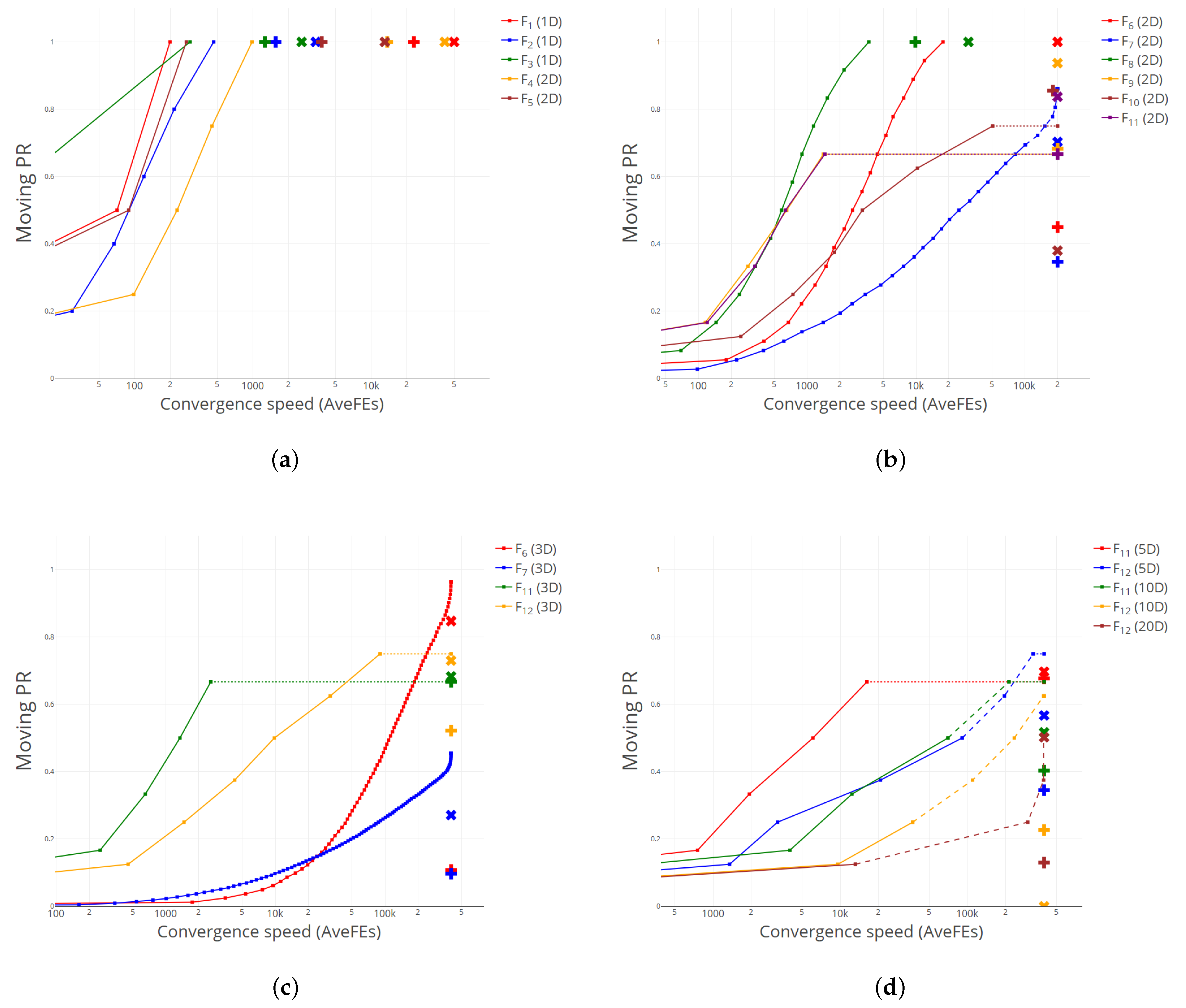
We can provide further insight into the good performance of CS compared to the baseline niching algorithms examining the values of the two new metrics mPR and mSR defined in Section 3.1. The available information in [34] for DE1 and DE2 is the average PR attained and the average number of FEs spent, computed over the NR = 50 runs and for an accuracy level $ϵ={10}^{-4}$. We have plotted these values in Figure 1, using plus and cross symbols for DE1 and DE2, respectively. Note that we have used a logarithmic scale on the abscissa axis for a better visualization. For the ease of viewing, we present four different plots, grouping the test functions according to their MaxFEs budget. Specifically, Figure 1a (MaxFEs = 50,000) displays functions $F_1$ to $F_5$; Figure 1b (MaxFEs = 200,000), $F_6$–$F_{11}$ (all 2D); Figure 1c (MaxFEs = 400,000), $F_6$, $F_7$, $F_{11}$ and $F_{12}$ (all 3D); and Figure 1d (MaxFEs = 400,000), $F_{11}$ (5D and 10D) and $F_{12}$ (5D, 10D and 20D).

As for CS, we have represented the performance curves mPR vs. AveFEs with solid dots for each test function and for the same accuracy level $ϵ={10}^{-4}$.

We also want to keep track of the robustness of our methods, using the moving success rate mSR defined in Section 3.1. To that aim, we have adopted the following graphical convention—particularly well observed in Figure 1d—for the lines joining every two consecutive points within a performance curve: (1) A solid line, when the number of global optima found in every run coincides with the value of $\nu \left(\mathtt{mPR}\right)$ at the endpoint of the segment, i.e., when mSR = 1 in both extremes of the segment. Note, however, that, as long as $\mathtt{mPR}<1$ holds, different sets of global optima may have been found on different runs. (2) A dashed line, when only some runs found the number of global optima associated with $\nu \left(\mathtt{mPR}\right)$ at the endpoint, that is, when 0 < mSR < 1. In such cases, note that the average FE was computed by assigning the maximum value MaxFEs to the unsuccessful runs, as indicated in the competition rules. (3) A horizontal dotted line extending as far as MaxFEs, meaning that no more global optima were found on any run within the available budget, that is mSR = 0. Note that, for the sake of clarity, we have clipped in each graphic the region between $\nu \left(\mathtt{mPR}\right)=0$ and $\nu \left(\mathtt{mPR}\right)=1$.

In consequence, if for a given test function, the associated performance curve lies above the corresponding plus and/or cross symbols, it means that CS has outperformed DE1 and/or DE2, respectively, in terms of PR, and vice versa. In the limiting case when the maximum value of the performance curve coincides with the score of either niching algorithm, the success rate SR and the convergence speed would be used as ancillary criteria, as indicated in [34] and reflected in Table 1.

As we can observe, CS attains a great performance, particularly for the higher-dimensional functions, plotted in Figure 1c,d. For most test functions, the performance curve has a “full” sigmoidal shape, which points at the ability of CS to find new global optima in a steady and relatively fast way, leaving the scores of DE1 and DE2 far behind to its right in the plot. Only for some of the “hardest” functions in Figure 1c,d the performance curve is somehow flattened, exhibiting only the convex part of the sigmoidal trend, something which is indicative of how tough it becomes to find new global optima across convoluted and high-dimensional functions. However, even for these challenging cases, the accomplishment of CS is remarkable, ensuring a consistent discovery rate of new global optima—see, for instance $F_6$ (3D) and $F_7$ (3D)—something that is probably boosted by the suitable random generation strategy chosen in our setting.

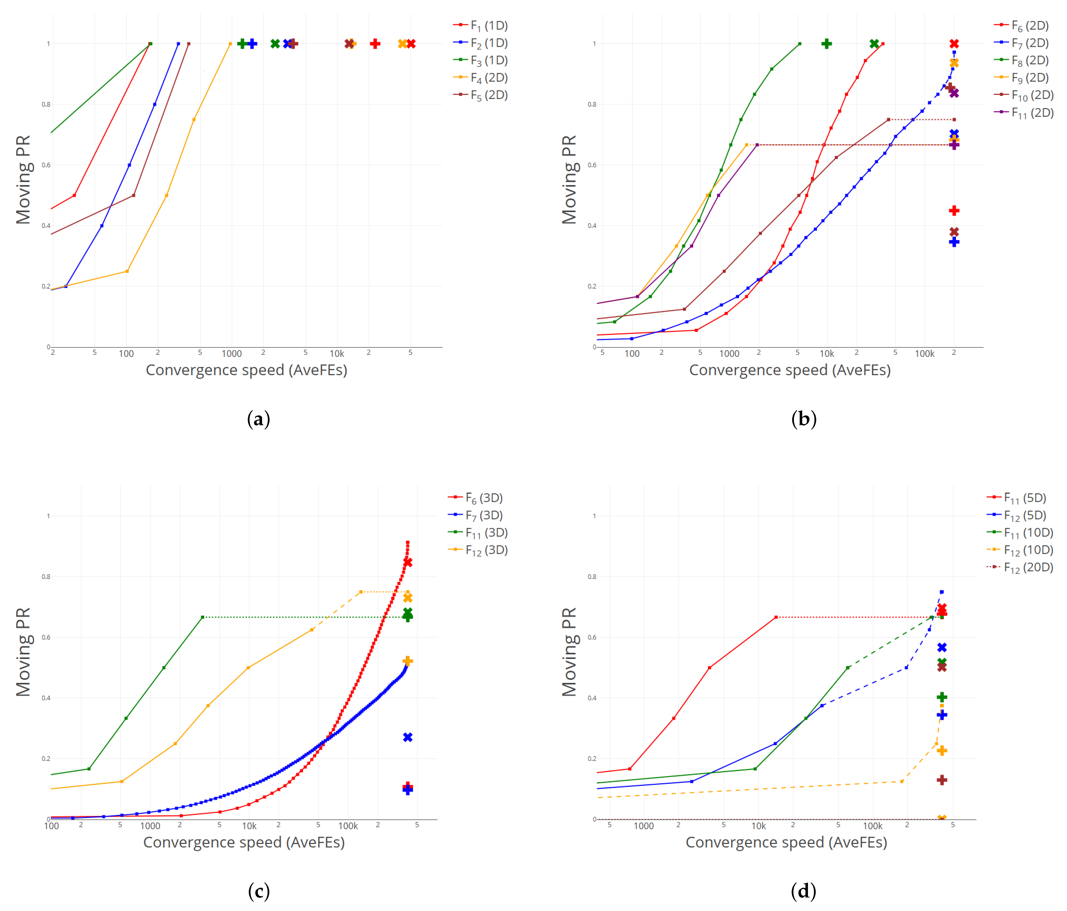
5.2. Simplex Search Methods: Nelder-Mead

We comment now more briefly the results obtained by NM, as a germane example of the performance of simplex search methods, which was implemented using the following parameters: the initial size of the simplex edges was set to 1, whereas the contraction, expansion, and reflection coefficients were set to 0.5, 2 and 1, respectively. We used two termination criteria in the final step: (i) The vector distance moved is fractionally smaller in magnitude than ${10}^{-4}$. (ii) The increase in the function value is fractionally smaller than $ϵ$.

Table 2. PR, SR and convergence speed ($ϵ=$${10}^{-4}$) for NM.

	${\mathit{F}}_1$(1D)		${\mathit{F}}_2$(1D)		${\mathit{F}}_3$(1D)		${\mathit{F}}_4$(2D)		${\mathit{F}}_5$(2D)
Accuracy Level$\mathbf{ϵ}$	PR	SR	PR	SR	PR	SR	PR	SR	PR	SR
${10}^{-1}$	1.000	1.000	1.000	1.000	1.000	1.000	1.000	1.000	1.000	1.000
${10}^{-2}$	0.02	0.000	1.000	1.000	1.000	1.000	1.000	1.000	1.000	1.000
${10}^{-3}$	0.02	0.000	1.000	1.000	1.000	1.000	1.000	1.000	1.000	1.000
${10}^{-4}$	0.05	0.000	1.000	1.000	1.000	1.000	1.000	1.000	1.000	1.000
Convergence speed	50,000.0	0.000	446.0	189.987	370.0	348.013	565.0	249.638	288.0	144.609
${10}^{-5}$	0.004	0.00	1.000	1.000	1.000	1.000	1.000	1.000	1.000	1.000
	${\mathit{F}}_{\mathbf{6}}$(2D)		${\mathit{F}}_{\mathbf{7}}$(2D)		${\mathit{F}}_{\mathbf{6}}$(3D)		${\mathit{F}}_{\mathbf{7}}$(3D)		${\mathit{F}}_{\mathbf{8}}$(2D)
Accuracy Level  $\mathbf{ϵ}$	PR	SR	PR	SR	PR	SR	PR	SR	PR	SR
${10}^{-1}$	0.998	0.960	0.886	0.000	0.385	0.000	0.676	0.000	1.000	1.000
${10}^{-2}$	0.991	0.980	0.882	0.000	0.397	0.000	0.667	0.000	1.000	1.000
${10}^{-3}$	1.000	1.000	0.884	0.000	0.412	0.000	0.679	0.000	1.000	1.000
${10}^{-4}$	0.998	0.960	0.887	0.000	0.389	0.000	0.674	0.000	1.000	1.000
Convergence speed	44,975.0	34,213.793	200,000.0	0.000	400,000.0	0.000	400,000.0	0.000	4935.0	2589.305
${10}^{-5}$	0.997	0.980	0.870	0.000	0.192	0.000	0.680	0.000	1.000	1.000
	${\mathit{F}}_{\mathbf{9}}$(2D)		${\mathit{F}}_{\mathbf{10}}$(2D)		${\mathit{F}}_{\mathbf{11}}$(2D)		${\mathit{F}}_{\mathbf{11}}$(3D)		${\mathit{F}}_{\mathbf{12}}$(3D)
Accuracy Level  $\mathbf{ϵ}$	PR	SR	PR	SR	PR	SR	PR	SR	PR	SR
${10}^{-1}$	1.000	1.000	0.997	0.980	0.997	0.980	0.680	0.000	0.733	0.000
${10}^{-2}$	1.000	1.000	0.000	1.000	0.983	0.900	0.667	0.000	0.733	0.000
${10}^{-3}$	1.000	1.000	1.000	1.000	0.987	0.920	0.667	0.000	0.707	0.000
${10}^{-4}$	1.000	1.000	1.000	1.000	0.993	0.960	0.667	0.000	0.733	0.000
Convergence speed	6877.0	5065.769	65,671.0	46,501.38	65,151.0	54,227.57	400,000.0	0.000	400,000.0	0.000
${10}^{-5}$	1.000	1.000	0.997	0.980	0.977	0.860	0.667	0.000	0.655	0.000
	${\mathit{F}}_{\mathbf{11}}$(5D)		${\mathit{F}}_{\mathbf{12}}$(5D)		${\mathit{F}}_{\mathbf{11}}$(10D)		${\mathit{F}}_{\mathbf{12}}$(10D)		${\mathit{F}}_{\mathbf{12}}$(20D)
Accuracy Level  $\mathbf{ϵ}$	PR	SR	PR	SR	PR	SR	PR	SR	PR	SR
${10}^{-1}$	0.667	0.000	0.502	0.000	0.353	0.000	0.045	0.000	0.000	0.000
${10}^{-2}$	0.667	0.000	0.462	0.000	0.373	0.000	0.052	0.000	0.000	0.000
${10}^{-3}$	0.667	0.000	0.490	0.000	0.370	0.000	0.052	0.000	0.000	0.000
${10}^{-4}$	0.667	0.000	0.465	0.000	0.193	0.000	0.010	0.000	0.000	0.000
Convergence speed	400,000.0	0.000	400,000.0	0.000	400,000.0	0.000	400,000.0	0.000	400,000.0	0.000
${10}^{-5}$	0.317	0.000	0.130	0.000	0.000	0.000	0.000	0.000	0.000	0.000

presents the results for NM. As we can observe, the performance is also remarkable, when compared to the baseline niching algorithms DE1 and DE2, and very close to that of CS. As for the improvement in the number of function evaluations, big reductions are again achieved.

Figure 2 shows the performance curves for NM, compared to the average results obtained by DE1 and DE2 for an accuracy level $ϵ=$10⁻⁴. Again, we can see that most plus and cross symbols lie below and to the right of the corresponding curve, illustrating the excellent results obtained by NM.

It is worth mentioning that CS and NM seem to have a complementary behavior, in the sense that NM obtains better results precisely in those functions where CS finds more difficulties, like $F_9$ (2D), $F_{10}$ (2D) or $F_{11}$ (2D), and vice versa: CS stands out in some of the functions where NM attains its poorest results, e.g., $F_{12}$ (10D or 20D). This is an interesting feature, that could be exploited by e.g., devising some kind of hybrid strategy, where different direct search methods could be used when restarting the algorithm, trying to get advantage of their different abilities to find global optima.

5.3. Rosenbrock’s Method

Finally, we present the results obtained when using RB. The vector of initial steplenghts was set to 20% of the range of each dimension, being multiplied by a factor of 3 in case of a successful step, and by −0.5, otherwise. The minimum steplength was fixed at ${10}^{-4}$.

Table 3. PR, SR and convergence speed ($ϵ=$${10}^{-4}$) for RB.

	${\mathit{F}}_1$(1D)		${\mathit{F}}_2$(1D)		${\mathit{F}}_3$(1D)		${\mathit{F}}_4$(2D)		${\mathit{F}}_5$(2D)
Accuracy Level  $\mathbf{ϵ}$	PR	SR	PR	SR	PR	SR	PR	SR	PR	SR
${10}^{-1}$	1.000	1.000	1.000	1.000	1.000	1.000	1.000	1.000	1.000	1.000
${10}^{-2}$	1.000	1.000	1.000	1.000	1.000	1.000	1.000	1.000	1.000	1.000
${10}^{-3}$	1.000	1.000	1.000	1.000	1.000	1.000	1.000	1.000	1.000	1.000
${10}^{-4}$	1.000	1.000	1.000	1.000	1.000	1.000	1.000	1.000	1.000	1.000
Convergence speed	163.0	126.861	311.0	138.230	170.0	156.255	966.0	541.892	389.0	246.292
${10}^{-5}$	1.000	1.000	1.000	1.000	1.000	1.000	1.000	1.000	1.000	1.000
	${\mathit{F}}_{\mathbf{6}}$(2D)		${\mathit{F}}_{\mathbf{7}}$(2D)		${\mathit{F}}_{\mathbf{6}}$(3D)		${\mathit{F}}_{\mathbf{7}}$(3D)		${\mathit{F}}_{\mathbf{8}}$(2D)
Accuracy Level  $\mathbf{ϵ}$	PR	SR	PR	SR	PR	SR	PR	SR	PR	SR
${10}^{-1}$	1.000	1.000	0.889	0.020	0.896	0.000	0.515	0.000	1.000	1.000
${10}^{-2}$	1.000	1.000	0.856	0.000	0.896	0.000	0.505	0.000	1.000	1.000
${10}^{-3}$	1.000	1.000	0.864	0.000	0.891	0.000	0.503	0.000	1.000	1.000
${10}^{-4}$	1.000	1.000	0.863	0.000	0.832	0.000	0.492	0.000	1.000	1.000
Convergence speed	37,156.0	15,930.223	200,000.0	0.000	400,000.0	0.000	400,000.0	0.000	5223.0	2967.538
${10}^{-5}$	1.000	1.000	0.859	0.000	0.097	0.000	0.482	0.000	1.000	1.000
	${\mathit{F}}_{\mathbf{9}}$(2D)		${\mathit{F}}_{\mathbf{10}}$(2D)		${\mathit{F}}_{\mathbf{11}}$(2D)		${\mathit{F}}_{\mathbf{11}}$(3D)		${\mathit{F}}_{\mathbf{12}}$(3D)
Accuracy Level  $\mathbf{ϵ}$	PR	SR	PR	SR	PR	SR	PR	SR	PR	SR
${10}^{-1}$	0.680	0.000	0.768	0.000	0.667	0.000	0.667	0.000	0.782	0.020
${10}^{-2}$	0.667	0.000	0.750	0.000	0.667	0.000	0.667	0.000	0.750	0.000
${10}^{-3}$	0.667	0.000	0.750	0.000	0.667	0.000	0.667	0.000	0.750	0.000
${10}^{-4}$	0.667	0.000	0.750	0.000	0.667	0.000	0.667	0.000	0.748	0.000
Convergence speed	200,000.0	0.000	200,000.0	0.000	200,000.0	0.000	400,000.0	0.000	400,000.0	0.000
${10}^{-5}$	0.667	0.000	0.680	0.000	0.667	0.000	0.667	0.000	0.432	0.000
	${\mathit{F}}_{\mathbf{11}}$(5D)		${\mathit{F}}_{\mathbf{12}}$(5D)		${\mathit{F}}_{\mathbf{11}}$(10D)		${\mathit{F}}_{\mathbf{12}}$(10D)		${\mathit{F}}_{\mathbf{12}}$(20D)
Accuracy Level  $\mathbf{ϵ}$	PR	SR	PR	SR	PR	SR	PR	SR	PR	SR
${10}^{-1}$	0.907	0.540	0.740	0.120	0.673	0.040	0.182	0.000	0.002	0.000
${10}^{-2}$	0.667	0.000	0.592	0.000	0.593	0.000	0.182	0.000	0.000	0.000
${10}^{-3}$	0.667	0.000	0.585	0.000	0.570	0.000	0.170	0.000	0.000	0.000
${10}^{-4}$	0.667	0.000	0.550	0.000	0.567	0.000	0.140	0.000	0.000	0.000
Convergence speed	400,000.0	0.000	400,000.0	0.000	400,000.0	0.000	400,000.0	0.000	400,000.0	0.000
${10}^{-5}$	0.667	0.000	0.432	0.000	0.587	0.000	0.050	0.000	0.000	0.000

displays the records for PR, SR and FE. As we can observe, RB attains remarkable results in the three metrics. Specifically, it wins (ties) in 35% (42%) of the cases in terms of PR, and in 8% (81%) of them when the measure of interest is SR. As for the convergence speed, the performance is equally good, winning (tying) in 35% (60%) of the cases, with large reductions in the number of FE of up to 99% in $F_1$, outperforming the already excellent results of CS.

Figure 3 shows the performance curves for RB. As we can observe, more often than not, such curves lie above the corresponding points of DE1 and DE2, and/or leave them to their right, meaning that RB is able to achieve better or equal results than DE1/DE2 in terms of PR spending, in approximately one third of the cases, less FE.

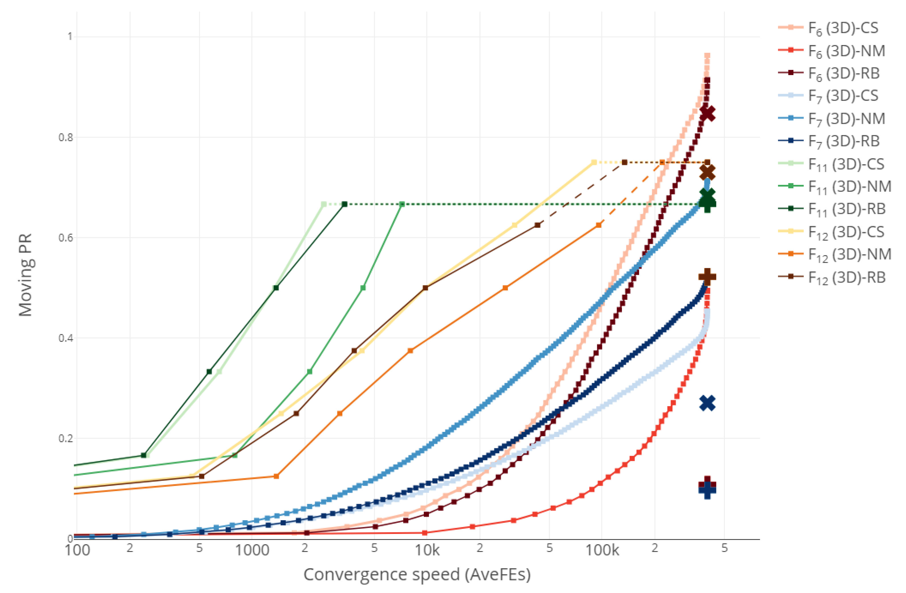
5.4. Comparison between Direct Search Methods

We finish our analysis of the obtained results comparing the performance curves of the three direct methods considered. For the sake of brevity and clarity, we only present the plot for functions $F_6$, $F_7$, $F_{11}$, $F_{12}$ (all 3D) in Figure 4, although graphics for the other functions are given as Supplementary Material at https://www.mdpi.com/article/10.3390/math10091494/s1 (accessed on 20 Janurary 2022). Note that Figure 4 simply merges Figure 1c, Figure 2c and Figure 3c but provides a better visualization. We have grouped the 12 performance curves by color, using the palettes Reds for $F_6$, Blues for $F_7$, Greens for $F_{11}$ and YlOrBr for $F_{12}$, as specified in https://cran.r-project.org/web/packages/RColorBrewer (accessed on 21 Janurary 2022). We have also included the PR values obtained by DE1 (plus) and DE2 (cross).

As it can be seen, CS (plotted with the lighter color in the palette) attains the best results for three of the four functions considered, performing worse than NM or RB only on $F_7$. A similar behavior was observed for the other clusters of functions displayed on subplots (a), (b) and (d) of Figure 1, Figure 2 and Figure 3. This is in accordance with what was already reflected in Table 1, Table 2 and Table 3, where the superiority of CS compared to NM and RB was evident. Nevertheless, rather than comparing direct search methods in an attempt to highlight their differences, we believe it would be more worth it to combine them in some way or another to take advantage of their complementary features and behaviors. That will be the subject of future research.

Finally, we have also compared the performance of the different direct search methods in an attempt to assess whether there are significant differences between them. In other words, we are interested in discerning whether the values of PR and SR might depend on the choice of a particular local search algorithm. To that aim, we performed a one-way ANOVA test on the number of distinct global optima found by each direct search method on each run. The results obtained suggested that there were significant differences between the three direct search methods analyzed, as indicated by their low p-values.

6. Conclusions

Multimodal optimization (MMO) problems, far from being a mathematical extravagance, arise in real-life examples from many areas of sciences and engineering. In these problems, the goal is to find multiple optimal solutions—either global or local—so that a better knowledge about different optimal solutions in the search space can be gained.

Although MMO problems have been attracting attention since the last decade of the 20th century, they are experiencing a revival in recent years. However, the focus has almost exclusively been put on meta-heuristic algorithms, particularly on evolutionary algorithms, evolutionary strategies, particle swarm optimization and differential evolution. These methods have proved notably effective in solving MMO problems—in terms of accurately locate and robustly maintain multiple optima—when equipped with the diversity preserving mechanisms typical of niching methods.

We propose in this paper a radically different approach, based on the exclusive use of local search methods. Among the wealth of such methods, we have chosen direct search methods, in their most basic implementation, as our optimization tool. Unlike more traditional optimization methods that use first- or second-order information to search for local optima, direct search methods investigate a set of points around the current one, looking for improvements in the objective function based purely on function evaluations.

We have tried different methods belonging to the three basic families within direct search methods: (1) pattern search, (2) simplex search, and (3) methods with adaptive sets of directions. We have tested such methods on the set of benchmark functions proposed in the 2013 Competition on Niching Methods for Multimodal Optimization. The results obtained for all the relevant performance metrics described in [34]—peak ratio, success rate and convergence speed—are remarkable when compared to the two baseline niching algorithms provided therein. We have proposed two new performances measures—the so-called moving peak ratio and moving success rate—that study the accomplishment of the different methods in a dynamic way, focusing on how fast and reliably global optima are found as the available budget is depleted.

As far as we are aware, this is a pioneer strategy to solve MMO problems, and leaves the door open to further improvements. To wit, our numerical results suggest that it could be advisable to combine, in some way or another, different direct search methods within an overall restarting strategy, aiming to take advantage of the best of each method. That could be complemented with more advanced random generation techniques for sampling the initial seeds, dynamically detecting if certain regions in the search space are proving fruitless in the seek of new global optima, forcing the algorithm to quickly move away from them. Another promising area is the devise of more sophisticated line search procedures, benefiting from the local properties of the objective function. We are confident that our methods could be successfully used in practical applications.