Genetic Mean Reversion Strategy for Online Portfolio Selection with Transaction Costs

Abstract

Online portfolio selection (OLPS) is a procedure for allocating portfolio assets using only past information to maximize an expected return. There have been successful mean reversion strategies that have achieved large excess returns on the traditional OLPS benchmark datasets. We propose a genetic mean reversion strategy that evolves a population of portfolio vectors using a hybrid genetic algorithm. Each vector represents the proportion of the portfolio assets, and our strategy chooses the best vector in terms of the expected returns on every trading day. To test our strategy, we used the price information of the S&P 500 constituents from 2000 to 2017 and compared various strategies for online portfolio selection. Our hybrid genetic framework successfully evolved the portfolio vectors; therefore, our strategy outperformed the other strategies when explicit or implicit transaction costs were incurred.

1. Introduction

In equity markets, mean reversion assumes that stocks that recently produced higher-than-average returns will tend to generate lower-than-average returns, and vice versa. The overreaction hypothesis states that the mean reversion occurs when stock prices overreact to information [1]. In recent decades, there have been controversial findings on the existence of the mean reversion. Fama and French [2] found the evidence of negative autocorrelations in stock returns, Balvers et al. [3] provided the empirical support for the mean reversion across national stock markets, and Gropp [4] showed that it is possible to earn excess returns by exploiting the mean reversion property. However, Kim et al. [5] reported that evidence of mean reversion in U.S. stock returns was weak, and Booth et al. [6] suggested that mean reversion assumption is not needed because the small-firm effect alone can explain the anomaly.

In contrast to mean reversion, the momentum effect documented in Jegadeesh and Titman [7] states that stocks that have performed well in the past tend to generate better returns at 3 to 12-month horizons than stocks that have performed poorly in the past. Jegadeesh and Titman [8] demonstrated the existence of the momentum effect on the U.S. stock markets from 1965 to 1998, and Fama and French [9] found strong momentum returns in international stock markets. The momentum effect is attributable to investors’ delayed overreactions [8] or underreactions to new information [10].

Online portfolio selection (OLPS) is a procedure of selling stocks with low expected returns and purchasing stocks with high expected returns. OLPS aims to maximize cumulative return by periodically adjusting the weights of stocks in an portfolio using the historical prices of the stocks. There are two representative types of OLPS strategies. The follow-the-leader methods [11,12,13] pursue the best strategy so far, whereas the follow-the-loser methods [14,15,16,17] exploit the mean reversion property. Refer to [18] for a comprehensive survey of he OLPS.

There are three types of mean reversion strategy that outperform other OLPS strategies on traditional benchmark datasets: a passive aggressive mean reversion (PAMR) strategy [15], an online moving average reversion (OLMAR) strategy [16], and a transaction cost optimization (TCO) strategy [17]. The PAMR uses the daily prices of a stock to determine if the stock is mean-revertible, whereas OLMAR utilizes the moving average of daily prices. The TCO can use either the daily prices or the moving average of daily prices to exploit the mean reversion property.

Investors pay transaction costs when they trade securities. Explicit transaction costs include taxes and commissions, and implicit transaction costs include price-impact costs and bid–ask spreads. Based on institutional trading data, Keim and Madhavan [19] found that explicit and implicit transaction costs were at least 0.13% and 0.11%, respectively. They also reported that the total transaction costs incurred by the transaction initiators were at least 0.26% on the New York Stock Exchange (NYSE) and NYSE American. As transaction costs depend on the trading volume, it is desirable to avoid unnecessary transactions.

The genetic algorithm (GA) is a metaheuristic inspired by biological evolution. To simulate natural selection, the GA evolves a population of candidate solutions through selection, crossover, mutation, and replacement operations. The behavior of GA is determined by the exploration and exploitation relationship [20]. Here, exploration is the process of visiting entirely new regions of a search space, and exploitation is the process of visiting the neighborhood of previously visited regions [21]. The GA has many successful real-world applications, including bioinformatics [22,23], operational research [24,25], medical image processing [26,27], and financial engineering [28,29,30].

The GA has been used extensively to solve the Markowitz mean-variance portfolio optimization problem [31], which maximizes expected return while minimizing risk. For example, Chang et al. [32] used GA to find the cardinality constrained efficient frontier, Skolpadungket et al. [33] compared various multi-objective GAs for solving portfolio optimization with multiple constraints, Chen et al. [34] proposed a non-dominated sorting and local search based multi-objective evolutionary framework to solve cardinality constrained portfolio optimization, and Kalayci et al. [35] used a hybrid metaheuristic that embeds GAs to find the cardinality-constrained efficient frontier.

A GA hybridized with a local search heuristic is called a hybrid GA (HGA). Using an HGA, we propose a mean reversion strategy for an OLPS. The HGA uses historical price information to evolve a population of portfolio vectors representing proportions of portfolio assets, and our strategy selects the most prominent mean-revertible vector on every trading day. We tested our strategy using 10 datasets from S&P 500, and compared the results with those obtained using state-of-the-art mean reversion strategies from other researches [15,16,17]. We believe that this is the first application of GA to OLPS.

The rest of this paper is organized as follows: In Section 2, we present some preliminaries on OLPS. In Section 3, we provide the details of the genetic mean reversion strategy. In Section 4, we present the experimental setup and results. Finally, in Section 5, we draw some concluding remarks and discuss future research directions.

2. Preliminaries

Let m be the number of securities in a portfolio, and n be the number of total trading days. On the $t^{\mathrm{th}}$ day, the closing prices of the securities are represented by ${\mathbf{p}}_t=(p_t\left(1\right),p_t\left(2\right),...,p_t\left(m\right))\in {\mathbb{R}}_{+}^m$, where $p_t\left(i\right)$ is the closing price of the $i^{\mathrm{th}}$ security. The daily returns of the securities are represented by a price relative vector, ${\mathbf{x}}_t=(x_t\left(1\right),x_t\left(2\right),...,x_t\left(m\right))\in {\mathbb{R}}_{+}^m$, where $x_t\left(i\right)=p_t\left(i\right)/p_{t-1}\left(i\right)$. Before the start of the $t^{\mathrm{th}}$ trading day, we decide a portfolio vector, ${\mathbf{b}}_t=(b_t\left(1\right),b_t\left(2\right),...,b_t\left(m\right))\in {\mathbb{R}}_{+}^m$, where $b_t\left(i\right)$ denotes the weight of the $i^{\mathrm{th}}$ security and ${\sum }_{i=1}^m{b}_t\left(i\right)=1$. After the $t^{\mathrm{th}}$ trading day, the daily return is calculated as ${\mathbf{b}}_t·{\mathbf{x}}_t$, and the cumulative return for the n trading days is calculated as ${\prod }_{t=1}^n{\mathbf{b}}_t·{\mathbf{x}}_t$.

The objective of OLPS is to maximize the cumulative return for investors. We assume that all securities can be divided into fractional shares that can be traded at their closing prices on every trading day. These notation and assumptions are common in OLPS studies [11,13,15,16,17,36].

A buy-and-hold strategy (${\mathrm{BAH}}_{\mathbf{b}}$) is a passive strategy in which an investor buys stocks according to the portfolio vector $\mathbf{b}$ on the first day and holds them for the entire period. The uniform BAH is denoted by ${\mathrm{BAH}}_{\mathbf{U}}$, where $\mathbf{U}=(1/m,...,1/m)$. A constant rebalanced portfolio (${\mathrm{CRP}}_{\mathbf{b}}$) is a strategy that reallocates the wealth of the investor according to the portfolio vector $\mathbf{b}$ on every trading day. In hindsight, the best portfolio vector ${\mathbf{b}}^{*}$ for CRP can be determined as follows:

$$\begin{array}{c}\hfill \begin{array}{cc}\hfill {\mathbf{b}}^{*}& =\underset{\mathbf{b}\in {\mathbb{R}}_{+}^m}{arg\; max}\prod _{t=1}^n\mathbf{b}·{\mathbf{x}}_t\hfill \\ \hfill & {\mathrm{subject}\mathrm{to}\parallel \mathbf{b}\parallel }_1=1.\hfill \end{array}\end{array}$$

(1)

Universal portfolios (UPs) [11] asymptotically achieve the performance of ${\mathbf{b}}^{*}$ by dividing its initial wealth among all possible CRPs. Good approximation algorithms can efficiently implement a UP [37,38]. In this study, ${\mathrm{BAH}}_{\mathbf{U}}$ and a UP were used as benchmark measures of performance.

Passive aggressive mean reversion (PAMR) [15] exploits the single-period mean reversion because it generates the next portfolio vector using ${\mathbf{x}}_t$, the daily returns of stocks in the portfolio. The PAMR utilizes the passive aggressive online learning algorithm [39] to generate the next portfolio vector that is mean-revertible and close to the current portfolio vector; that is,

$$\begin{array}{c}\hfill \begin{array}{cc}\hfill {\mathbf{b}}_{t+1}& =\underset{\mathbf{b}\in {\mathbb{R}}_{+}^m}{arg\; min}\frac{1}{2}{\parallel \mathbf{b}-{\mathbf{b}}_t\parallel }^2\hfill \\ \hfill & \mathrm{subject}\mathrm{to}\mathbf{b}·{\mathbf{x}}_t\le ϵ\hfill \\ \hfill & {\parallel \mathbf{b}\parallel }_1=1.\hfill \end{array}\end{array}$$

(2)

To benefit from the single-period reversion ($\mathbf{b}·{\mathbf{x}}_t\le ϵ$), this strategy seeks a portfolio vector whose latest return is confined to $ϵ$. We set $ϵ$ to 0.5 as in Li et al. [15].

Another state-of-the-art mean reversion strategy is online moving average reversion (OLMAR) [16], which is a multi-period mean reversion strategy. Unlike PAMR, the OLMAR uses a simple moving average (SMA) to generate the next portfolio vector. The SMA is the arithmetic average of the closing prices. Here, ${\mathbf{SMA}}_t\left(w\right)\in {\mathbb{R}}_{+}^m$ denotes the SMA on the $t^{\mathrm{th}}$ day; that is,

$$\begin{array}{c}\hfill \begin{array}{c}\hfill {\mathbf{SMA}}_t\left(w\right)=\frac{1}{w}\sum _{i=t-w+1}^t{\mathbf{p}}_i,\end{array}\end{array}$$

(3)

where $w\in {\mathbb{Z}}_{+}$ is the window length. The OLMAR produces the next portfolio vector that is mean-revertible and close to the current portfolio vector; that is,

$$\begin{array}{c}\hfill \begin{array}{cc}\hfill {\mathbf{b}}_{t+1}=& \underset{\mathbf{b}\in {\mathbb{R}}_{+}^m}{arg\; min}\frac{1}{2}{\parallel \mathbf{b}-{\mathbf{b}}_t\parallel }^2\hfill \\ \hfill \mathrm{subject}\mathrm{to}& \mathbf{b}·{\tilde{\mathbf{x}}}_{t+1}\ge ϵ\mathrm{and}{\parallel \mathbf{b}\parallel }_1=1,\hfill \end{array}\end{array}$$

(4)

where $ϵ\in {\mathbb{R}}_{+}$ is the reversion threshold, and ${\tilde{\mathbf{x}}}_{t+1}\in {\mathbb{R}}_{+}^m$ is the predicted relative price; that is,

$$\begin{array}{c}\hfill \begin{array}{c}\hfill {\tilde{\mathbf{x}}}_{t+1}\left(w\right)={\mathbf{SMA}}_t\left(w\right)\oslash {\mathbf{p}}_t,\end{array}\end{array}$$

(5)

where ⊘ represents the Hadamard (element-wise) division. As in Li et al. [16], we set $ϵ$ to 10 and w to 5.

The other state-of-the-art mean reversion strategy is the transaction cost optimization (TCO) [17], which aims to perform well even in the presence of non-zero transaction costs. The TCO does not allow trivial trades to reduce transaction costs. Let $\widehat{{\mathbf{b}}_t}\in {\mathbb{R}}_{+}^m$ be the closing price adjusted portfolio vector on the the $t^{\mathrm{th}}$ day, and ${\tilde{\mathbf{b}}}_{t+\frac{1}{2}}\in {\mathbb{R}}^m$ be the proportions to be reallocated after the $t^{\mathrm{th}}$ day. The TCO then uses the predicted relative price to calculate ${\tilde{\mathbf{b}}}_{t+\frac{1}{2}}$; that is,

$$\begin{array}{c}\hfill {\tilde{\mathbf{b}}}_{t+\frac{1}{2}}=\eta \left(\frac{{\tilde{\mathbf{x}}}_{t+1}}{\widehat{{\mathbf{b}}_t}·{\tilde{\mathbf{x}}}_{t+1}}-\frac{1}{m}\mathbf{1}·\frac{{\tilde{\mathbf{x}}}_{t+1}}{\widehat{{\mathbf{b}}_t}·{\tilde{\mathbf{x}}}_{t+1}}\right),\end{array}$$

(6)

where ${\widehat{\mathbf{b}}}_t=({\mathbf{b}}_t\odot {\mathbf{x}}_t)/\left({\mathbf{b}}_t·{\mathbf{x}}_t\right)$, ⊙ denotes the Hadamard (element-wise) product, and $\eta \in {\mathbb{R}}_{+}$ is a smoothing parameter. The positive elements of ${\tilde{\mathbf{b}}}_{t+\frac{1}{2}}$ have above-average expected returns, and thus their weights will be increased on the ${(t+1)}^{\mathrm{th}}$ day day, and vice versa; that is,

$$\begin{array}{c}\hfill b_{t+1}\left(i\right)={\widehat{b}}_t\left(i\right)+\left(\mathbb{I}\left[{\tilde{b}}_{t+\frac{1}{2}}\left(i\right)\ge 0\right]-\mathbb{I}\left[{\tilde{b}}_{t+\frac{1}{2}}\left(i\right)<0\right]\right)·max\left(\left|{\tilde{b}}_{t+\frac{1}{2}}\left(i\right)\right|-\lambda ,0\right),\end{array}$$

(7)

for all $1\le i\le m$, where $\lambda \in {\mathbb{R}}_{+}$ is a trade-off parameter. Only changes larger than $\lambda$ are used to determine the next portfolio vector. We set $\eta$ to 10 and $\lambda$ to $10\times \eta \times \gamma$, where $\gamma$ is the transaction cost rate. (Li et al. [17] stated that they set $\lambda$ to $10\times \gamma$. However, their implementation set $\lambda$ to $10\times \eta \times \gamma$, which produces better results than $10\times \gamma$ and coincides with the results of their study.) As the elements of ${\mathbf{b}}_{t+1}$ may not summed to 1, ${\mathbf{b}}_{t+1}$ needs to be normalized; that is,

$$\begin{array}{c}\hfill \begin{array}{cc}\hfill {\mathbf{b}}_{t+1}& =\underset{\mathbf{b}\in {\mathbb{R}}_{+}^m}{arg\; min}{\parallel \mathbf{b}-{\mathbf{b}}_{t+1}\parallel }^2\hfill \\ \hfill & {\mathrm{subject}\mathrm{to}\parallel \mathbf{b}\parallel }_1=1.\hfill \end{array}\end{array}$$

(8)

The TCO calculates the predictive relative prices using either the single-period or the multi-period mean reversion property. The TCO-1 uses the daily returns, whereas TCO-2 utilizes the moving average of closing prices; that is,

$$\begin{array}{c}\hfill {\tilde{\mathbf{x}}}_{t+1}=\left\{\begin{array}{cc}\mathbf{1}\oslash {\mathbf{x}}_t\hfill & \mathrm{in}\mathrm{TCO}-1\hfill \\ {\mathbf{SMA}}_t\left(5\right)\oslash {\mathbf{x}}_t\hfill & \mathrm{in}\mathrm{TCO}-2.\hfill \end{array}\right.\end{array}$$

(9)

3. Methods

We used a steady-state hybrid genetic algorithm (HGA), whose pseudocode is given in Algorithm 1. Each individual is represented by a real-valued chromosome, which is a portfolio vector $\mathbf{b}\in {\mathbb{R}}_{+}^m$. The chromosome is a point in the m-dimensional simplex ${\Delta }_m$, specifying the proportions of a portfolio with m assets. We set the population size to 100 and generated the initial population by sampling 100 chromosomes uniformly from ${\Delta }_m$. The population of candidate portfolio vectors evolved through a hybrid genetic framework.

Algorithm 1 The outline of our HGA.

1: Create an initial population P  2: for$t\leftarrow 2$ to n do                                                                                                        ▷n is the last trading day  3:     FitnessUpdate(P, ${\mathbf{x}}_{t-1}$, ${\mathbf{x}}_t$)  4:     $(\mathbf{parent}\mathbf{1},\mathbf{parent}\mathbf{2})\leftarrow (\mathrm{Select}(P,{\mathbf{x}}_t),\mathrm{Select}(P,{\mathbf{x}}_t$))  5:     $(\mathbf{offspring}\mathbf{1},\mathbf{offspring}\mathbf{2})\leftarrow \mathrm{Crossover}(\mathbf{parent}\mathbf{1},\mathbf{parent}\mathbf{2})$  6:     Mutation($\mathbf{offspring}\mathbf{1},\mathbf{offspring}\mathbf{2}$)  7:     $\mathbf{offspring}\leftarrow$ LocalSearch($\mathbf{offspring}\mathbf{1},\mathbf{offspring}\mathbf{2},{\mathbf{x}}_t$)  8:     Replace(P, $\mathbf{offspring}$)

3.1. Fitness Update

Financial returns are assumed to be log-normal [40], and the objective of the portfolio optimization is often set to maximize the expected log return [18,41]. Therefore, we used the expected relative log return as the fitness of a chromosome. The benchmark of the relative log return is a uniform portfolio vector $\mathbf{u}=(1/m,...,1/m)$, which has the average return of all assets in the portfolio.

The uniform portfolio vector $\mathbf{u}$ also provides a baseline indicating whether each chromosome is mean-revertible on the $t^{\mathrm{th}}$ day. Let $\mathbf{c}\in {\Delta }_m$ be a chromosome and ${\mathbf{x}}_{t-1}$ be the relative price vector on the ${(t-1)}^{\mathrm{th}}$ day. If the return of $\mathbf{c}$ is less than that of $\mathbf{u}$, i.e., $\mathbf{c}·{\mathbf{x}}_{t-1}<\mathbf{u}·{\mathbf{x}}_{t-1}$, $\mathbf{c}$ is mean-revertible on the $t^{\mathrm{th}}$ day because its recent performance is below the benchmark; otherwise, it is trend following on the $t^{\mathrm{th}}$ day.

To effectively exploit the mean reversion property, we maintain two versions of fitness for a chromosome: the mean-revertible fitness and trend-following fitness. Each fitness is the expected relative log return parameterized by the mean and standard deviation, which are initialized to 0. The mean-revertible fitness is used to select a promising individual for a crossover, and the trend-following fitness is used to find an undesirable individual that needs to be replaced.

When ${\mathbf{x}}_t$ is revealed, $log\frac{\mathbf{c}·{\mathbf{x}}_t}{\mathbf{u}·{\mathbf{x}}_t}$ incrementally updates the parameters of the fitness, mean-revertible chromosomes update their own mean-revertible fitness, and trend-following chromosomes update their own trend-following fitness. The pseudocode of the fitness-updating procedure is given in Algorithm 2. Here, ${\mu }_m\left(\mathbf{c}\right)$ and ${\sigma }_m\left(\mathbf{c}\right)$ are the mean and standard deviation of the mean-revertible chromosome $\mathbf{c}$, and ${\mu }_n\left(\mathbf{c}\right)$ and ${\sigma }_n\left(\mathbf{c}\right)$ are those of the trend-following chromosome $\mathbf{c}$.

Algorithm 2 FitnessUpdate $(P,{\mathbf{x}}_{t-1},{\mathbf{x}}_t)$.

1: for each$\mathbf{c}\in P$do  2:     rtn $\leftarrow log\frac{\mathbf{c}·{\mathbf{x}}_t}{\mathbf{u}·{\mathbf{x}}_t}$                                                                                                  ▷ relative log return  3:     if $\mathbf{c}·{\mathbf{x}}_{t-1}<\mathbf{u}·{\mathbf{x}}_{t-1}$ then                                                    ▷ for mean-revertible chromosomes  4:         Update ${\mu }_m\left(\mathbf{c}\right),{\sigma }_m\left(\mathbf{c}\right)$ incrementally using rtn  5:     else                                                                                           ▷ for trend-following chromosomes  6:         Update ${\mu }_n\left(\mathbf{c}\right),{\sigma }_n\left(\mathbf{c}\right)$ incrementally using rtn

3.2. Selection

For the genetic algorithm, the selection is the source of exploitation [42], which is the ability of the algorithm to move toward the direction of desired improvement [43]. After each $t^{\mathrm{th}}$ trading day, we select two prominent mean-revertible chromosomes as parents for later breeding. Only chromosomes that produced below-average returns on the t^th day were considered. The fitness of the chromosome is its expected relative log return when it is mean-revertible. To obtain the mean-revertible fitness of a chromosome $\mathbf{c}$, we sample a relative log return from $\mathcal{N}({\mu }_m\left(\mathbf{c}\right),{\sigma }_m^2\left(\mathbf{c}\right))$, using the Box-Muller transform [44]. The pseudocode of the selection function is given in Algorithm 3.

Algorithm 3 Select $(P,{\mathbf{x}}_t$).

1: $best\leftarrow -\infty$                                                                                                 ▷$best$ stores the best fitness  2: for each $\mathbf{c}\in P$do  3:     if $\mathbf{c}·{\mathbf{x}}_t<\mathbf{u}·{\mathbf{x}}_t$ then                                                                  ▷ test whether $\mathbf{c}$ is mean-revertible  4:         Sample $rtn\sim \mathcal{N}({\mu }_m\left(\mathbf{c}\right),{\sigma }_m^2\left(\mathbf{c}\right))$  5:         if $rtn>best$ then  6:            $(best,\mathbf{b})\leftarrow (rtn,\mathbf{c})$                                                              ▷$\mathbf{b}$ stores the fittest chromosome  7: if$best=-\infty$then  8:     Randomly sample $\mathbf{b}\sim P$                                                     ▷ all chromosomes are trend following  9: return$\mathbf{b}$

3.3. Crossover and Mutation

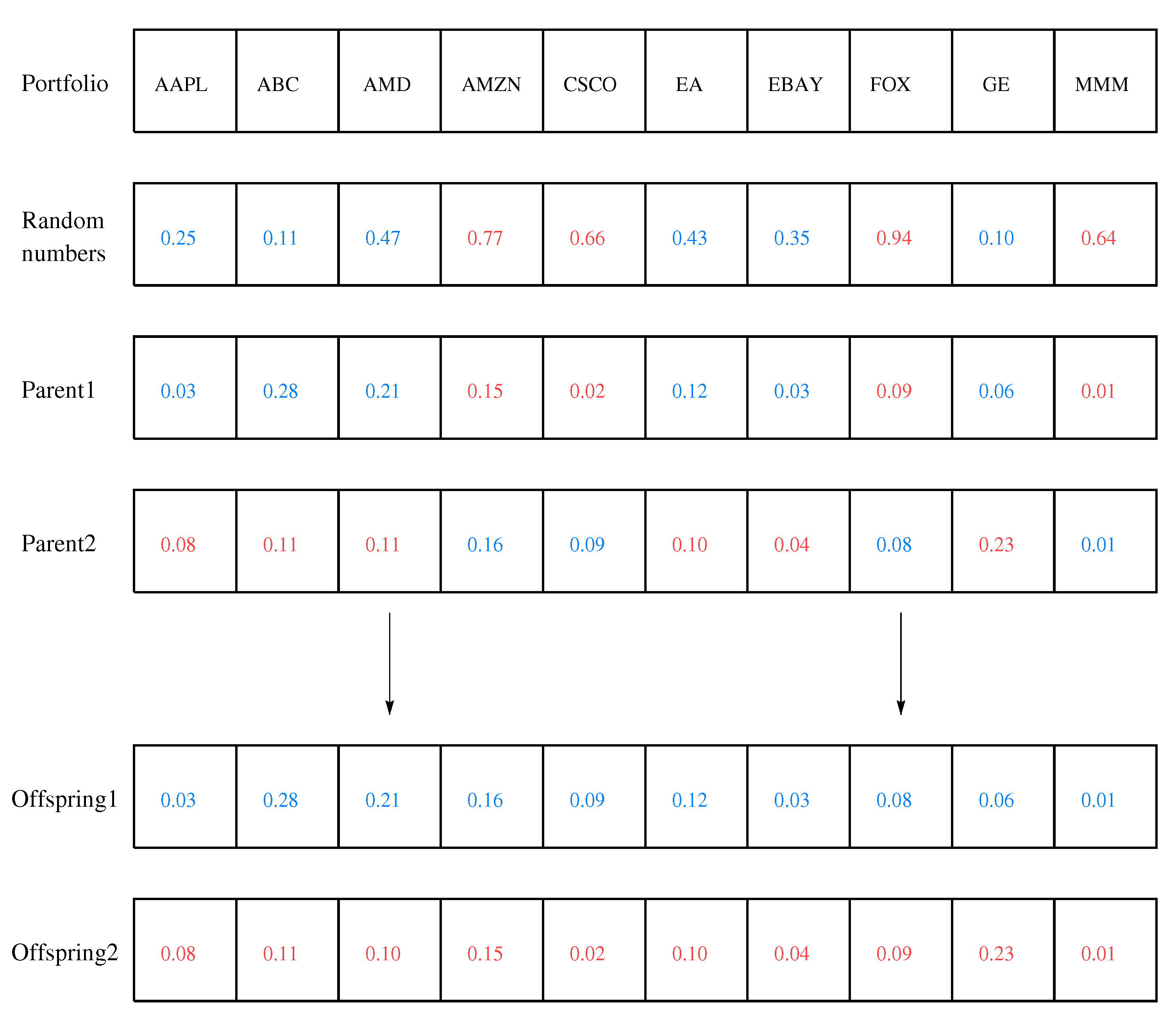
A crossover combines two parents to create new offspring. We used a uniform crossover in which each gene was inherited from either parent with equal probability. Figure 1 shows an example of a uniform crossover, which results in two offspring. The crossover is exploitative because it recombines the material of promising parents; however, it is also explorative because it generates new offspring [42].

After a crossover, each offspring undergoes a mutation. The mutation rate was set to $\mu$, and the mutated gene was multiplied by $(1+\beta )$ or $(1-\beta )$. The multiplicand was randomly selected with the same probability. We set $\mu$ to 0.05 and $\beta$ to 0.5. A mutation can also be seen as both explorative and exploitative because it introduces new offspring in an unbiased manner while conserving most of the original chromosome [42].

3.4. Local Search Heuristic

The GA can explore a wide range of search spaces using explorative operators when the hyperparameters are appropriately set. However, it is weak in fine-tuning capability near the local or global optima, which can be alleviated by HGA [45]. Thus, we incorporated a local search heuristic into the GA to improve the fine-tuning capability.

We first generated two additional chromosomes by taking the inverse of each gene in the two offspring. We then manipulated each gene of the two offspring and the two new chromosomes. On the $t^{\mathrm{th}}$ day, each $i^{\mathrm{th}}$ gene in the four chromosomes is multiplied by $(1+\beta )$ if the return of the $i^{\mathrm{th}}$ stock is below average; otherwise, it is multiplied by $(1-\beta )$. We set $\beta$ to 0.5.

This heuristic makes the chromosomes perform worse on the $t^{\mathrm{th}}$ day, which strengthens the mean reversion property on the next day. Each chromosome $\mathbf{c}$ is normalized such that it belongs to the simplex—that is, $\mathbf{c}=\mathbf{c}/{\parallel \mathbf{c}\parallel }_1$—and the best mean-revertible chromosome is chosen for replacement. The pseudocode of the local search heuristic is given in Algorithm 4.

Algorithm 4 LocalSearch ($\mathbf{offspring}\mathbf{1},\mathbf{offspring}\mathbf{2},{\mathbf{x}}_t$).

1: $avg\leftarrow {\sum }_{i=1}^m{x}_t\left(i\right)/m$                                                                            ▷$avg$ stores the average return  2: for$i\leftarrow 1$ to m do  3:     $chromosome1\left(i\right)\leftarrow offspring1{\left(i\right)}^{-1}$                                                 ▷$c\left(i\right)$ denotes the $i^{\mathrm{th}}$ gene  4:     $chromosome2\left(i\right)\leftarrow offspring2{\left(i\right)}^{-1}$  5: $C\leftarrow \{\mathbf{offspring}\mathbf{1},\mathbf{offspring}\mathbf{2},\mathbf{chromosome}\mathbf{1},\mathbf{chromosome}\mathbf{2}\}$  6: for$i\leftarrow 1$ to m do  7:     if $x_t\left(i\right)<avg$ then  8:         for each $\mathbf{c}\in C$ do  9:            $c\left(i\right)\leftarrow c\left(i\right)*(1+\beta )$  10:     else  11:         for each $\mathbf{c}\in C$ do  12:            $c\left(i\right)\leftarrow c\left(i\right)*(1-\beta )$  13: for each$\mathbf{c}\in C$do  14:     $\mathbf{c}=\mathbf{c}/{\parallel \mathbf{c}\parallel }_1$                                                                                                                      ▷ normalization  15: $\mathbf{b}\leftarrow argmi{n}_{\mathbf{c}\in C}\mathbf{c}·{\mathbf{x}}_t$                                                    ▷ select the best mean-revertible chromosome  16: return$\mathbf{b}$

3.5. Replacement

The mean reversion property expects the current best strategy to fail. Therefore, we replace the best trend-following chromosome with the best mean-revertible chromosome. On the $t^{\mathrm{th}}$ day, we choose an individual only from the chromosomes that produce above-average returns. The fitness of a chromosome is its expected relative log return when it is trend following. To obtain the trend-following fitness of a chromosome $\mathbf{c}$, we sample a relative log return from $\mathcal{N}({\mu }_n\left(\mathbf{c}\right),{\sigma }_n^2\left(\mathbf{c}\right))$. The pseudocode of the replacement procedure is given in Algorithm 5.

Algorithm 5 Replace $(P,\mathbf{offspring}$).

1: $best\leftarrow -\infty$                                                                                                              ▷$best$ stores the best fitness  2: for each$\mathbf{c}\in P$do  3:     if $\mathbf{c}·{\mathbf{x}}_t\ge \mathbf{u}·{\mathbf{x}}_t$ then                                                                   ▷ test whether $\mathbf{c}$ is trend following or not  4:         Sample $rtn\sim \mathcal{N}({\mu }_n\left(\mathbf{c}\right),{\sigma }_n^2\left(\mathbf{c}\right))$  5:         if $rtn>best$ then  6:            $(best,\mathbf{b})\leftarrow (rtn,\mathbf{c})$                                                  ▷$\mathbf{b}$ stores the best trend-following chromosome  7: if$best=-\infty$then  8:     Randomly sample $\mathbf{b}\sim P$                                                                 ▷ all chromosomes are mean-revertible  9: $P\leftarrow (P\setminus \{\mathbf{b}\left\}\right)\cup \left\{\mathbf{offspring}\right\}$

3.6. Genetic Mean Reversion Strategy

Our strategy starts with a uniform portfolio vector—that is, ${\mathbf{b}}_1=(1/m,...,1/m)$. After the $t^{\mathrm{th}}$ day, a new portfolio vector is generated by combining the previous portfolio vector with the most promising mean-revertible vector in the population P; that is,

$$\begin{array}{c}\hfill {\mathbf{b}}_{t+1}=(1-\alpha ){\mathbf{b}}_t+\alpha \underset{\mathbf{c}\in P}{arg\; min}\mathbf{c}·{\mathbf{x}}_t,\end{array}$$

(10)

where $\alpha$ is a user-defined parameter that prevents excessive trading. We set $\alpha$ to $\frac{0.0005}{\gamma \delta }$, where $\gamma$ is the transaction cost rate and $\delta =\parallel {\mathbf{b}}_t{-\mathbf{c}\parallel }_1$. As $\gamma \delta$ is proportional to the actual transaction cost of changing the portfolio vector from ${\mathbf{b}}_t$ to $\mathbf{c}$, $\alpha$ is set adaptively to reduce the transaction costs. We set $\alpha$ to 1 when there is no transaction cost.

Our hybrid genetic framework maintains profitable individuals with the mean reversion property and tries to achieve higher returns than the benchmarks by selecting the most mean-revertible portfolio vector according to the market conditions. The results of our strategy are compared with those of previous state-of-the-art mean reversion strategies [15,16,17].

4. Results

4.1. Data

We used the historical daily prices of the companies in the S&P 500 from 2000 to 2017. This dataset contains 389 stocks with price information for the entire period. The dataset was used in our preliminary study [46], and generated in the following way: the stocks were sorted in alphabetical order based on their ticker symbols, and 10 portfolios were generated sequentially in that order. To the best of our knowledge, this is the largest dataset used in an OLPS study. Our dataset is summarized in

Table 1. Summary of the S&P 500 dataset.

Name	Period	Days	Stocks a	Max (${\mathit{x}}_{\mathit{t}}\left(\mathit{j}\right)$) b	Min (${\mathit{x}}_{\mathit{t}}\left(\mathit{j}\right)$) c
SP500(0)	2000–2017	4527	39	1.6600	0.3921
SP500(1)	2000–2017	4527	39	1.5782	0.5494
SP500(2)	2000–2017	4527	39	1.6296	0.5402
SP500(3)	2000–2017	4527	39	1.6037	0.4133
SP500(4)	2000–2017	4527	39	2.0236	0.4844
SP500(5)	2000–2017	4527	39	1.5425	0.3948
SP500(6)	2000–2017	4527	39	1.8698	0.5873
SP500(7)	2000–2017	4527	39	1.7545	0.3195
SP500(8)	2000–2017	4527	39	1.5605	0.4096
SP500(9)	2000–2017	4527	38	2.0101	0.3811

^a The number of stocks in the portfolio. ^b The highest daily return on a stock in the portfolio. ^c The lowest daily return on a stock in the portfolio.

. (The dataset in .mat and .csv formats is available at the following address: https://github.com/uramoon/mr_dataset (Accessed on: 13 February 2022). A detailed description of the dataset is provided in the README file.) Appendix A presents the experimental results on the single portfolio of all 389 stocks.

We also tested our strategy using traditional datasets, which have been widely used by many researchers [12,14,15,36,47]. However, some of these datasets do not provide the criteria for stock selection [15] and have abnormal patterns that can be easily exploited using mean reversion strategies. Therefore, although we mainly used our own datasets, we also provide the details of traditional datasets and the experimental results using them in Appendix B.

4.2. Experimental Setup

The genetic mean reversion (GMR) strategy was written in C#, and the results of the GMR were averaged over 100 independent runs for all experiments. The averaged results can be implemented in the real market by splitting the initial wealth evenly among the 100 runs and prohibiting the transfer of money between runs [38]. When there are transaction costs, the average performance can be improved by offsetting trades among the runs [37].

For the other strategies, we used the implementations of Li et al. [16,17,48]. Here, ${\mathrm{BAH}}_{\mathbf{U}}$ and UP were used as benchmark measures of performance. We also compared our strategy with the state-of-the-art mean reversion strategies: PAMR, OLMAR, TCO-1, and TCO-2 [15,16,17].

Even if there is no commission, traders incur an implicit cost in the difference between the actual transaction price and the benchmark price [49]. To incorporate all expenses that can be incurred in actual trading, we used the proportional commission model [36] in which an investor pays at a rate of $\gamma \in [0,1]$ for each buy and each sell such that the daily return on the $t^{\mathrm{th}}$ day is $\left({\mathbf{b}}_t·{\mathbf{x}}_t\right)\times (1-\gamma ·\parallel {\mathbf{b}}_t-{\widehat{\mathbf{b}}}_{t-1}{\parallel }_1$). Here, ${\widehat{\mathbf{b}}}_{t-1}$ is the closing price adjusted portfolio vector (i.e., ${\widehat{\mathbf{b}}}_{t-1}=({\mathbf{b}}_{t-1}\odot {\mathbf{x}}_{t-1})/\left({\mathbf{b}}_{t-1}·{\mathbf{x}}_{t-1}\right)$), and $\gamma$ is set to 0%, 0.25%, and 0.5%, which are reasonable transaction cost rates for OLPS [17,50]. The transaction on the t^th day is profitable only when the excess profit from the transaction (${\mathbf{b}}_t·{\mathbf{x}}_t-{\widehat{\mathbf{b}}}_{t-1}·{\mathbf{x}}_t$) outweighs the transaction costs ($\gamma ·\parallel {\mathbf{b}}_t-{\widehat{\mathbf{b}}}_{t-1}{\parallel }_1$).

Cumulative wealth at the end of the trading period is our main performance criterion. The cumulative wealth measures the wealth of a trading strategy with an initial wealth of 1. We also calculated the average daily turnover ratio ($0.5·\parallel {\mathbf{b}}_t-{\widehat{\mathbf{b}}}_{t-1}{\parallel }_1$) for each strategy, which denotes the mean ratio of assets that have been replaced on every trading day. As the transaction costs depend on the turnover ratio, it is desirable to avoid unnecessary transactions.

We also compare the results of GMR with those of ${\mathrm{BAH}}_{\mathbf{U}}$ in terms of annualized percentage yield (APY), annualized standard deviation (ASD), Sharpe ratio (SR), the maximum drawdown (MDD), alpha ($\alpha$), t-statistics, and p-value. The APY is annual compound return, and the ASD is the standard deviation of daily returns multiplied by the squared root of the number of annual trading days. The SR measures the risk-adjusted performance of a trading strategy compared to a risk-free asset, i.e., $\mathrm{SR}=(\mathrm{APY}-{\mathrm{R}}_f)/\mathrm{ASD}$, where ${\mathrm{R}}_f$ is the risk-free return (U.S. Treasury bill rate). The MDD is the maximum observed loss from a peak to a valley, which measures the downside risk over a certain period. $\alpha$ is the intercept from the market model regression [51] that measures the excess daily return of GMR against ${\mathrm{BAH}}_{\mathbf{U}}$. The t-statistic is the test statistic for the null hypothesis that the $\alpha$ is zero [52], and the p-value is computed from the t-statistic. A low p-value indicates that we can reject the null hypothesis.

4.3. Cumulative Wealth without Transaction Costs

We first conducted experiments to test the GMR strategy in the absence of the transaction costs. As transaction costs were not considered, it would be extremely difficult to achieve a similar performance in the real market.

Table 2. Cumulative wealth achieved by various strategies on the S&P 500 datasets. The transaction costs were not considered. The best values are shown in bold.

Data	Benchmarks		Previous Mean Reversion Strategies				GMR
	${\mathbf{BAH}}_{\mathit{U}}$	UP	PAMR	OLMAR	TCO-1	TCO-2
SP500(0)	9.44	13.45	1.52	0.18	2.14	2.29	28.77
SP500(1)	8.31	9.80	5.45	3.96	11.68	4.33	56.51
SP500(2)	6.97	8.54	198.24	176.03	232.07	353.57	62.35
SP500(3)	6.68	9.15	103.52	3564.62	230.16	189.85	46.25
SP500(4)	7.54	8.67	95.58	33.24	93.28	84.79	54.40
SP500(5)	6.39	7.76	162.52	169.98	191.22	316.48	39.86
SP500(6)	24.29	11.15	9.48	4.46	12.80	9.93	55.05
SP500(7)	7.92	11.95	16.24	14.67	40.62	73.39	58.35
SP500(8)	8.90	12.39	154.65	81.66	88.85	22.59	160.27
SP500(9)	6.49	9.16	101.82	103.66	52.32	155.14	103.03
Average	9.29	10.20	84.90	415.25	95.51	121.24	66.48
Turnover *	N/A	0.0159	0.8261	0.6191	0.5496	0.3333	0.5892
Win ratio **	N/A	N/A	0.7	0.7	0.8	0.7	1.0

* Average daily turnover ratio. ** The odds of winning against both benchmarks.

lists the cumulative wealth achieved using various strategies. The results of ${\mathrm{BAH}}_{\mathbf{U}}$ show that there is a strong upward trend in all datasets; the simple ${\mathrm{BAH}}_{\mathbf{U}}$ increased its wealth by over 6-fold on every dataset. The other benchmark UP improved the performance of ${\mathrm{BAH}}_{\mathbf{U}}$ overall with a small turnover ratio, but achieved less than half the wealth of ${\mathrm{BAH}}_{\mathbf{U}}$ on the SP500(6).

Although previous mean reversion strategies largely outperformed the benchmarks on many datasets, they showed a poor performance on the SP500(0), SP500(1), and SP500(6), all of which failed to beat ${\mathrm{BAH}}_{\mathbf{U}}$ on these three datasets, except for TCO-1, which performed better than ${\mathrm{BAH}}_{\mathbf{U}}$ on SP500(1). Although the OLMAR produced the best average performance by achieving tremendous wealth on SP500(3), it lost 82% of its wealth on SP500(0). In general, the multi-period mean reversion strategies (OLMAR and TCO-2) worked better than their single-period counterparts (PAMR and TCO-1) in terms of the average wealth and turnover ratio.

We also tested whether the results from GMR are significantly better than those from ${\mathrm{BAH}}_{\mathbf{U}}$.

Table 3. APY, ASD, SR, MDD, and $\alpha$, t-statistic, and p-value of GMR on the S&P 500 datasets. The transaction costs were not considered, and the p-value less than 0.05 are denoted with an asterisk.

Data	${\mathbf{BAH}}_{\mathit{U}}$				GMR
	APY	ASD	SR	MDD	APY	ASD	SR	MDD	$\mathit{\alpha }$	t-Statistics	p-Value
SP500(0)	0.1328	0.2092	0.5588	0.5503	0.2052	0.3158	0.5994	0.6921	0.0003	1.4095	0.0794
SP500(1)	0.1249	0.1979	0.5506	0.4695	0.2512	0.2875	0.8186	0.5313	0.0004	2.7085	$0.0034$ *
SP500(2)	0.1139	0.1940	0.5050	0.4850	0.2581	0.2601	0.9313	0.4606	0.0005	3.6514	$0.0001$ *
SP500(3)	0.1113	0.2002	0.4766	0.5211	0.2374	0.3030	0.7310	0.6308	0.0005	2.5172	$0.0059$ *
SP500(4)	0.1188	0.2123	0.4847	0.6277	0.2486	0.3013	0.7723	0.5351	0.0005	2.6804	$0.0037$ *
SP500(5)	0.1085	0.2143	0.4321	0.5838	0.2272	0.3169	0.6668	0.6203	0.0004	2.4057	$0.0081$ *
SP500(6)	0.1939	0.2643	0.6735	0.6226	0.2494	0.3460	0.6749	0.6455	0.0004	1.5566	0.0598
SP500(7)	0.1218	0.2067	0.5124	0.5013	0.2535	0.3899	0.6093	0.6403	0.0006	2.0393	$0.0207$ *
SP500(8)	0.1292	0.1911	0.5927	0.4974	0.3258	0.3546	0.8740	0.6797	0.0007	2.8101	$0.0025$ *
SP500(9)	0.1095	0.2007	0.4662	0.5566	0.2937	0.3323	0.8360	0.4898	0.0006	3.1257	$0.0009$ *

presents further details on the performance of both strategies. Although the GMR had higher risks (ASDs and MDDs) than ${\mathrm{BAH}}_{\mathbf{U}}$, it exhibited higher returns (APYs) and risk-adjusted returns (SRs) on all datasets. The p-values indicate that the excess returns ($\alpha$) of GMR against ${\mathrm{BAH}}_{\mathbf{U}}$ are statistically significant on the eight datasets.

Our method produced the best results on the four datasets SP500(0), SP500(1), SP500(6), and SP500(8), and outperformed the benchmarks on all datasets. To work well on unseen datasets, it is desirable to produce stable results on many different datasets. It is also worth noting that it showed the best results on the three datasets where the previous strategies failed to outperform the benchmarks. Although the average performance of GMR was below the previous strategies, its win ratio was the highest among the mean reversion strategies.

4.4. Cumulative Wealth with Transaction Costs

We tested the proposed strategy in the presence of transaction costs. The experimental results with reasonable transaction costs suggest how well each strategy will be applied in the real market.

Table 4. Cumulative wealth achieved by various strategies on the S&P 500 datasets. The transaction cost rate was 0.25%. The best values are shown in bold.

Data	Benchmarks		Previous Mean Reversion Strategies				GMR
	${\mathbf{BAH}}_{\mathit{U}}$	UP	PAMR	OLMAR	TCO-1	TCO-2
SP500(0)	9.41	9.18	0.00	0.00	0.01	0.04	25.73
SP500(1)	8.29	6.88	0.00	0.00	0.05	0.25	18.82
SP500(2)	6.95	5.92	0.00	0.00	1.07	5.19	9.19
SP500(3)	6.66	6.33	0.00	0.00	0.88	4.98	11.41
SP500(4)	7.52	6.04	0.00	0.00	0.43	1.55	13.38
SP500(5)	6.37	5.48	0.00	0.00	0.45	7.22	7.06
SP500(6)	24.23	7.69	0.00	0.00	0.07	0.62	24.00
SP500(7)	7.90	8.23	0.00	0.00	0.15	1.39	23.54
SP500(8)	8.88	8.69	0.00	0.00	0.09	0.19	18.96
SP500(9)	6.47	6.44	0.00	0.00	0.17	13.10	11.07
Average	9.27	7.09	0.00	0.00	0.34	3.45	16.32
Turnover *	N/A	0.0159	0.8271	0.6206	0.2057	0.1396	0.0027
Win ratio **	N/A	N/A	0.0	0.0	0.0	0.2	0.9

* Average daily turnover ratio. ** The odds of winning against both benchmarks.

shows the cumulative wealth achieved by various strategies when the transaction cost rate is 0.25%. The performance of ${\mathrm{BAH}}_{\mathbf{U}}$ barely changed because it pays the transaction costs only on the first day. However, the performance of UP was no better than ${\mathrm{BAH}}_{\mathbf{U}}$ on most datasets; the transaction costs of 0.25% outweighed the benefits of the asset reallocation.

Previous mean reversion strategies also did not perform well with transaction costs of 0.25%. The PAMR and OLMAR spent all their money on transaction costs because they did not consider the transaction costs when changing the portfolio vectors. The TCOs reduced their trading volumes by less than half, but failed to outperform the benchmarks on most datasets; TCO-2 performed the best on two datasets, but failed to outperform the benchmarks on the other eight datasets, and TCO-1 performed worse than the benchmarks on all datasets.

Similar to the previous mean reversion strategies, the transaction costs degraded the performance of the GMR. However, it achieved relatively good results by significantly reducing its turnover ratio and showed the best results on seven datasets, achieving the highest average earning and a win ratio of 0.9.

Table 5. APY, ASD, SR, MDD, and $\alpha$, t-statistic, and p-value of GMR on the S&P 500 datasets. The transaction cost rate was 0.25%, and the p-value less than 0.05 are denoted with an asterisk.

Data	${\mathbf{BAH}}_{\mathit{U}}$				GMR
	APY	ASD	SR	MDD	APY	ASD	SR	MDD	$\mathit{\alpha }$	t-Statistics	p-Value
SP500(0)	0.1326	0.2092	0.5580	0.5503	0.1977	0.2556	0.7113	0.5253	0.0002	2.0164	$0.0219$ *
SP500(1)	0.1247	0.1979	0.5498	0.4695	0.1771	0.2261	0.7129	0.4674	0.0002	2.3986	$0.0082$ *
SP500(2)	0.1137	0.1941	0.5041	0.4850	0.1312	0.2117	0.5444	0.5148	0.0001	0.9636	0.1677
SP500(3)	0.1111	0.2002	0.4757	0.5211	0.1448	0.2392	0.5391	0.6147	0.0001	1.2266	0.1100
SP500(4)	0.1186	0.2123	0.4839	0.6277	0.1550	0.2657	0.5236	0.6349	0.0002	1.1554	0.1240
SP500(5)	0.1084	0.2143	0.4314	0.5838	0.1147	0.2460	0.4016	0.6155	0.0000	0.3240	0.3730
SP500(6)	0.1937	0.2643	0.6728	0.6226	0.1931	0.2595	0.6830	0.6015	0.0001	0.9534	0.1702
SP500(7)	0.1217	0.2067	0.5116	0.5013	0.1918	0.2873	0.6121	0.5069	0.0003	1.6460	$0.0499$ *
SP500(8)	0.1290	0.1911	0.5918	0.4974	0.1776	0.2648	0.6106	0.5424	0.0002	1.1534	0.1244
SP500(9)	0.1093	0.2008	0.4654	0.5566	0.1429	0.2572	0.4937	0.5657	0.0001	0.9977	0.1592

compares GMR with ${\mathrm{BAH}}_{\mathbf{U}}$ when the transaction cost rate was set to 0.25%. Again, GMR had higher risks than ${\mathrm{BAH}}_{\mathbf{U}}$, but produced better annual returns and risk-adjusted returns on all datasets except SP500(5). On the nine datasets, GMR had positive excess daily returns, but they were statistically significant on three datasets in the presence of transaction costs.

We also tested the performance of each strategy with transaction costs of 0.5%.

Table 6. Cumulative wealth achieved by various strategies on the S&P 500 datasets. The transaction cost rate was 0.5%. The best values are shown in bold.

Data	Benchmarks		Previous Mean Reversion Strategies				GMR
	${\mathbf{BAH}}_{\mathit{U}}$	UP	PAMR	OLMAR	TCO-1	TCO-2
SP500(0)	9.39	6.43	0.00	0.00	0.00	0.03	24.14
SP500(1)	8.27	4.83	0.00	0.00	0.09	0.46	17.91
SP500(2)	6.93	4.19	0.00	0.00	0.86	4.60	8.88
SP500(3)	6.65	4.45	0.00	0.00	3.22	4.13	10.29
SP500(4)	7.51	4.24	0.00	0.00	0.36	2.29	12.80
SP500(5)	6.36	3.82	0.00	0.00	0.14	1.99	6.84
SP500(6)	24.17	5.30	0.00	0.00	0.20	1.35	24.82
SP500(7)	7.88	5.78	0.00	0.00	0.11	1.54	23.76
SP500(8)	8.86	6.20	0.00	0.00	0.05	0.11	18.59
SP500(9)	6.46	4.50	0.00	0.00	0.12	4.76	9.65
Average	9.25	4.97	0.00	0.00	0.51	2.13	15.77
Turnover *	N/A	0.0159	0.8281	0.6221	0.0920	0.0609	0.0014
Win ratio **	N/A	N/A	0.0	0.0	0.0	0.0	1.0

* Average daily turnover ratio. ** The odds of winning against both benchmarks.

lists the cumulative wealth achieved by the various strategies. The performance of ${\mathrm{BAH}}_{\mathbf{U}}$ barely changed. At this transaction cost rate, the UP and the previous mean reversion strategies did not exceed ${\mathrm{BAH}}_{\mathbf{U}}$ on all datasets. However, the GMR outperformed the benchmarks on all datasets by maintaining a good population of portfolio vectors and adaptively reducing the turnover ratio.

Table 7. APY, ASD, SR, MDD, and $\alpha$, t-statistic, and p-value of GMR on the S&P 500 datasets. The transaction cost rate was 0.5%, and the p-value less than 0.05 are denoted with an asterisk.

Data	${\mathbf{BAH}}_{\mathit{U}}$				GMR
	APY	ASD	SR	MDD	APY	ASD	SR	MDD	$\mathit{\alpha }$	t-Statistics	p-Value
SP500(0)	0.1325	0.2092	0.5572	0.5503	0.1935	0.2458	0.7225	0.5235	0.0002	2.1368	$0.0163$ *
SP500(1)	0.1245	0.1979	0.5489	0.4695	0.1739	0.2179	0.7249	0.4542	0.0002	2.6515	$0.0040$ *
SP500(2)	0.1136	0.1941	0.5033	0.4850	0.1290	0.2052	0.5512	0.5133	0.0001	1.0541	0.1460
SP500(3)	0.1110	0.2002	0.4749	0.5211	0.1382	0.2307	0.5304	0.5937	0.0001	1.1308	0.1291
SP500(4)	0.1185	0.2123	0.4831	0.6277	0.1522	0.2598	0.5245	0.6290	0.0002	1.1473	0.1257
SP500(5)	0.1082	0.2144	0.4306	0.5838	0.1128	0.2333	0.4152	0.6057	0.0000	0.3376	0.3679
SP500(6)	0.1936	0.2644	0.6721	0.6226	0.1953	0.2546	0.7049	0.6136	0.0001	0.9649	0.1673
SP500(7)	0.1215	0.2068	0.5108	0.5013	0.1924	0.2811	0.6280	0.5003	0.0003	1.7297	$0.0419$ *
SP500(8)	0.1288	0.1911	0.5909	0.4974	0.1763	0.2548	0.6295	0.5469	0.0002	1.2351	0.1084
SP500(9)	0.1092	0.2008	0.4646	0.5566	0.1342	0.2454	0.4823	0.5727	0.0001	0.8436	0.1995

shows that the risk-adjusted returns of GMR are overall higher than those of ${\mathrm{BAH}}_{\mathbf{U}}$ with transaction costs of 0.5%.

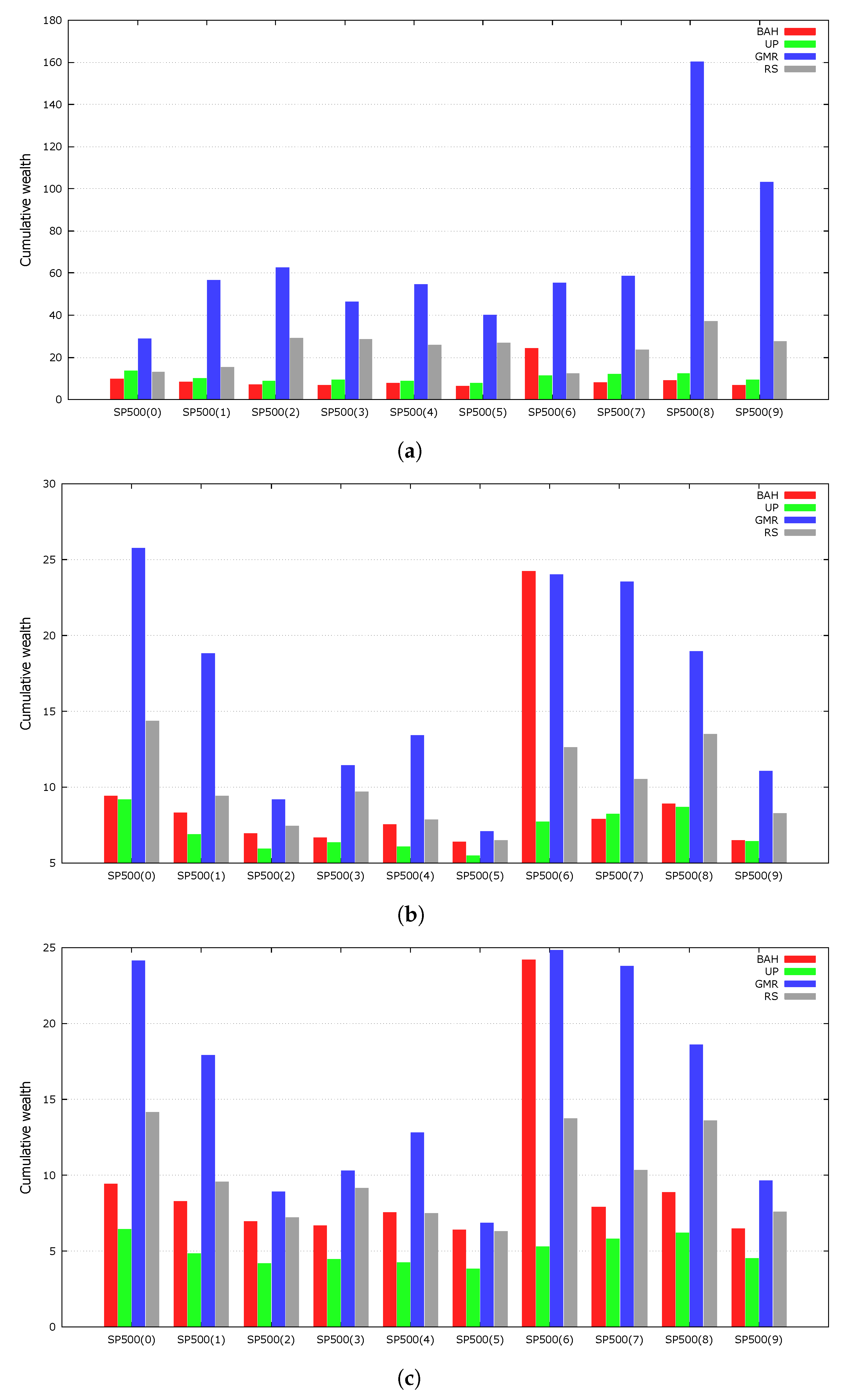
4.5. Comparisons of GA and Random Sampling

We compare a random sampling (RS) with a GA to examine how much the genetic framework contributes to the quality of the solutions. An RS is a population-based heuristic that produces a solution through random sampling. Instead of selecting two promising parents from the population, two individuals were uniformly sampled from the simplex. These individuals are processed through a local search, and the best solution replaces a random individual of the population. The RS results were averaged over 100 independent runs. The RS started with the same initial population as the GMR because it used the same random seed numbers as the GMR. Figure 2 presents the experimental results. The GMR outperformed the RS on every dataset, indicating that the GA successfully evolved the population of portfolio vectors.

4.6. Local Search Heuristic

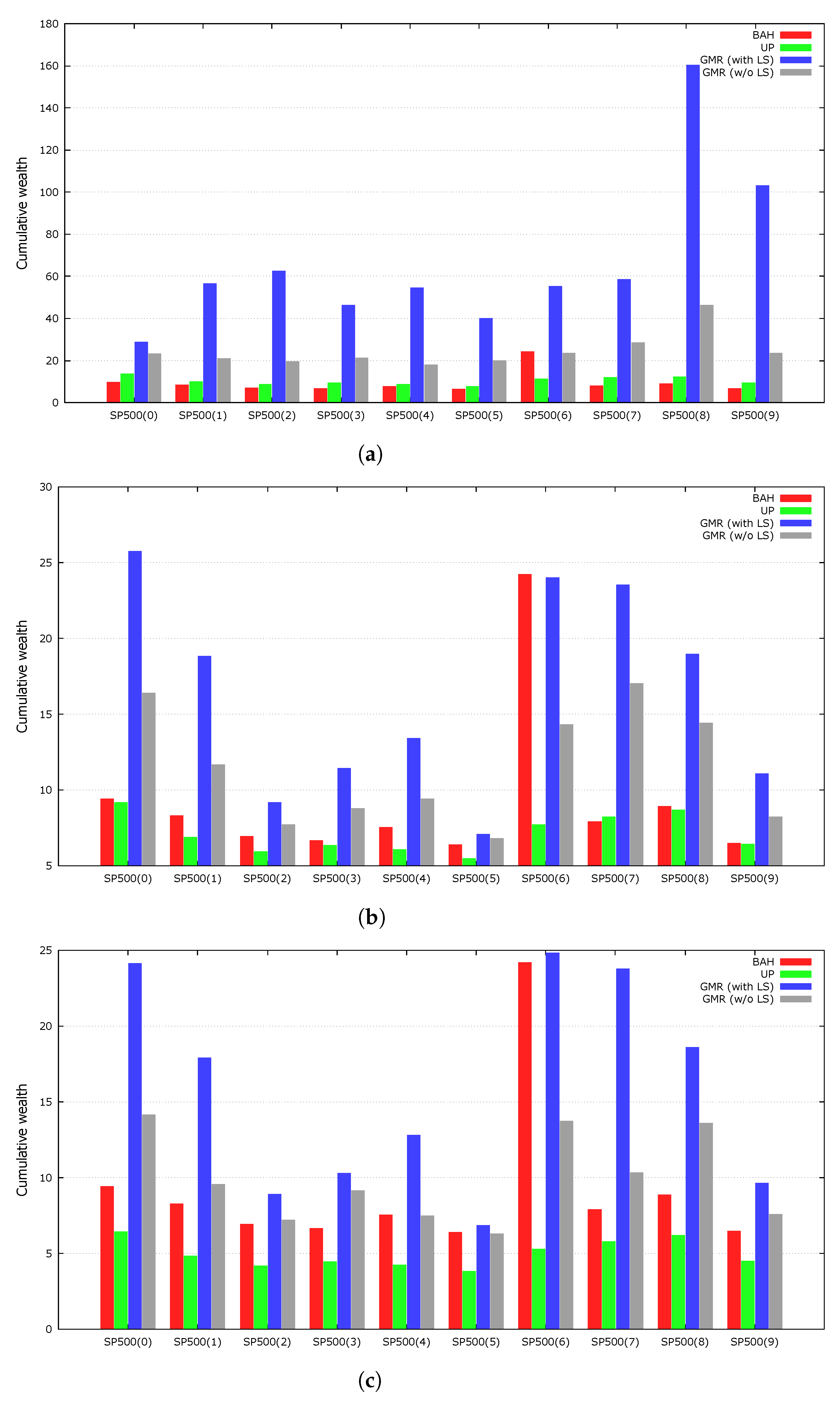
The GMR embeds a local search heuristic to improve the fine-tuning capability of the GA. To determine the effects of the local search, we tested the performance of GMR when not employing the local search heuristic. We averaged the results of the experiments over 100 independent runs using the same random seed numbers as the original GMR. Figure 3 shows the results of the experiments. The local search heuristic improved the performance of our genetic framework for every dataset.

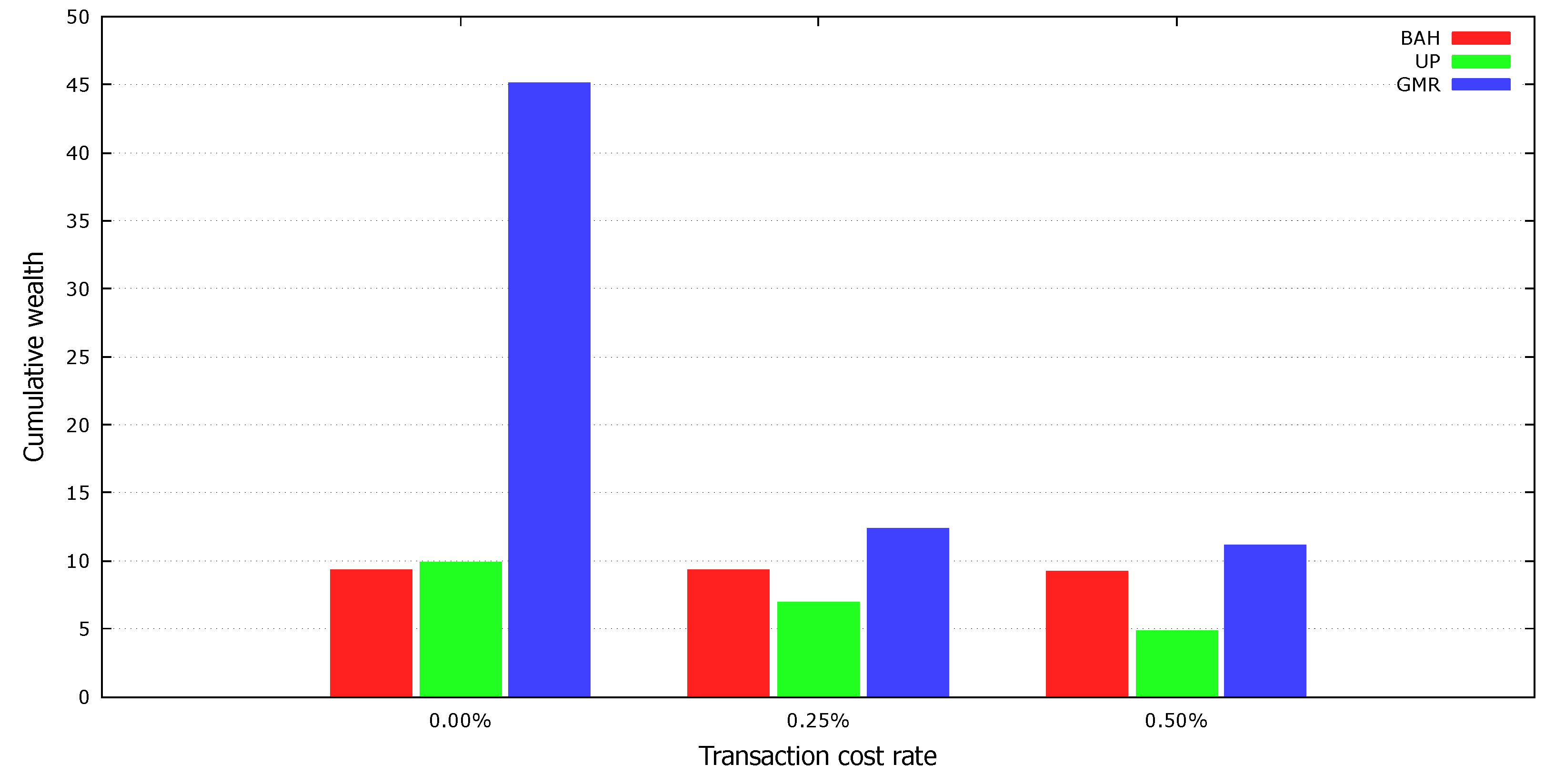
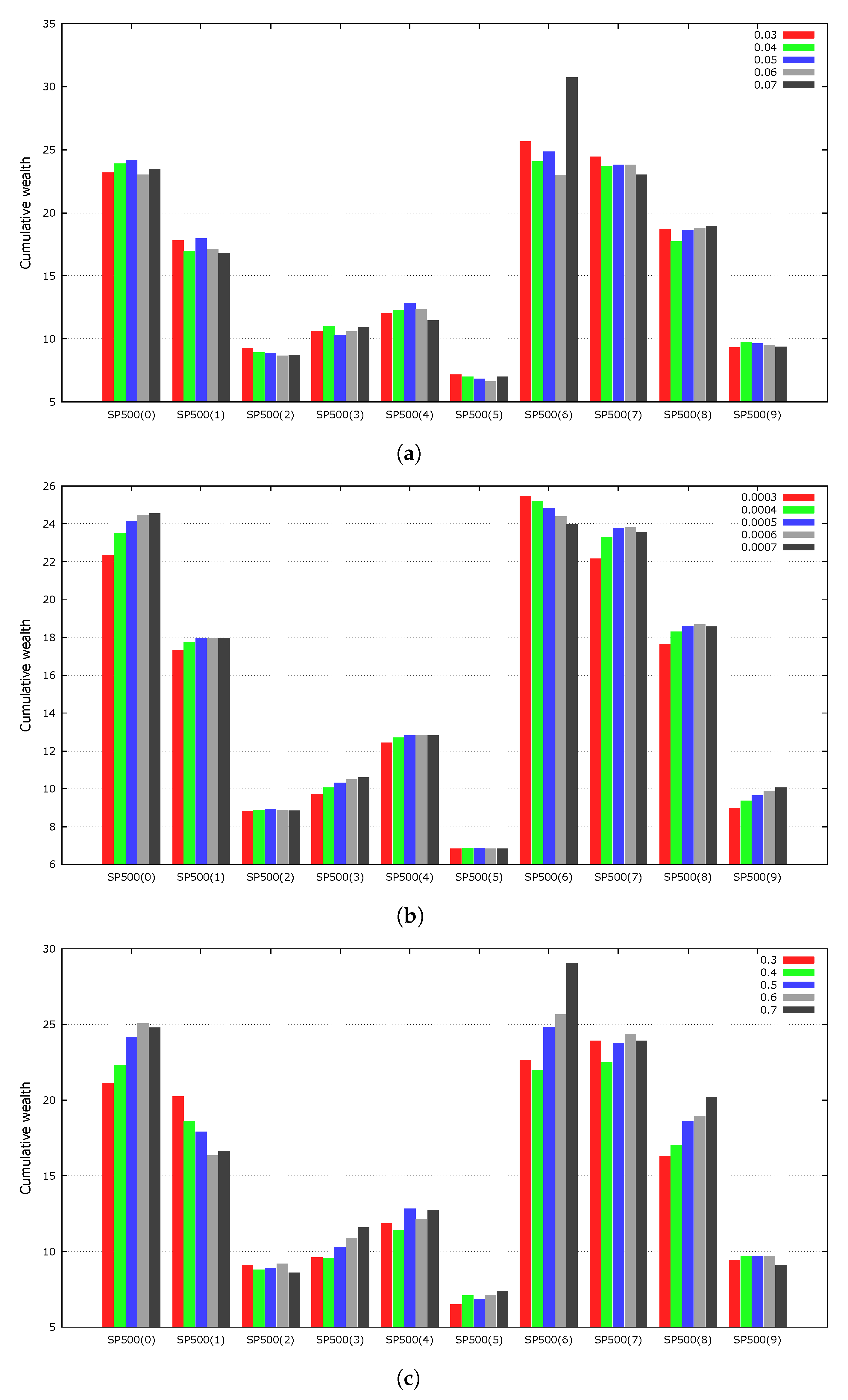
4.7. Parameter Sensitivity

Strategies that are highly sensitive to their parameters are not likely to perform well on unseen data. Experiments were conducted to determine the effect of the GMR parameters on the experimental results. We varied $\mu$, $\alpha$, and $\beta$, which mutation, portfolio vector calculation, and local search, respectively. For simplicity, we fixed the rate of transaction costs to 0.5% and averaged the results of the experiments over 100 independent runs. Figure 4 shows the experimental results. Overall, the value of each parameter did not significantly affect the experimental results. As OLPS is used for online algorithms, we deliberately did not fine-tune the parameters.

5. Conclusions

In this paper, we proposed a mean reversion strategy that evolves a population of portfolio vectors through the HGA. To exploit the mean reversion property, a local search heuristic was devised and embedded in the GA. The experimental results obtained for the S&P500 datasets revealed that our genetic framework and local search heuristic were able to improve the performance of our strategy.

We also investigated the performance of various mean reversion strategies on the S&P500 datasets. When there were no transaction costs, previous mean reversion strategies performed extremely well. However, they showed poor results with respect to the transaction costs. As our strategy limited the turnover ratio to an appropriate level based on the transaction costs, it outperformed the benchmarks on most of the datasets.

In the future, it would be worthwhile to develop a new strategy that incorporates both trend following and mean reversion disciplines. On the SP500(6) dataset, ${\mathrm{BAH}}_{\mathbf{U}}$ outperformed most of the mean reversion strategies; it might therefore, be helpful to adopt a trend following strategy by identifying the market conditions.