
A Dimension Group-Based Comprehensive Elite Learning Swarm Optimizer for Large-Scale Optimization

 , ,
, , 
Abstract
:1. Introduction
- (1)
- A dimension group-based comprehensive elite learning scheme is proposed to guide the update of inferior particles by learning from multiple superior ones. Instead of learning from only at most two exemplars in existing holistic large-scale PSOs [24,25,26,30], the devised learning strategy first randomly divides the dimensions of each inferior particle into several equally sized groups and then employs different superior particles to guide the update of different dimension groups. Moreover, unlike existing elite strategies that only use one elite to direct the evolution of an individual [43,44], it employs a random dimension group-based recombination techniques to try to integrate valuable evolutionary information in multiple elites to guide the update of each non-elite particle. In this way, the learning diversity of particles could be largely promoted, which is beneficial for particles to avoid falling into local traps. Moreover, it is also possible that useful evolutionary information embedded in different superior particles could be integrated to direct the learning of inferior particles, which may be profitable for particles to approach promising areas quickly.
- (2)
- Dynamic adjustment strategies for the control parameters involved in the proposed learning strategy are further designed to cooperate with the learning strategy to help PSO search the large-scale solution space properly. With these dynamic strategies, the developed DGCELSO could appropriately compromise the intensification and diversification of the search process at the swarm level and the particle level.
2. Related Work
2.1. Canonical PSO
2.2. Large-Scale PSO
2.2.1. Cooperative Coevolutionary Large-Scale PSO (CCPSO)
2.2.2. Holistic Large-Scale PSO
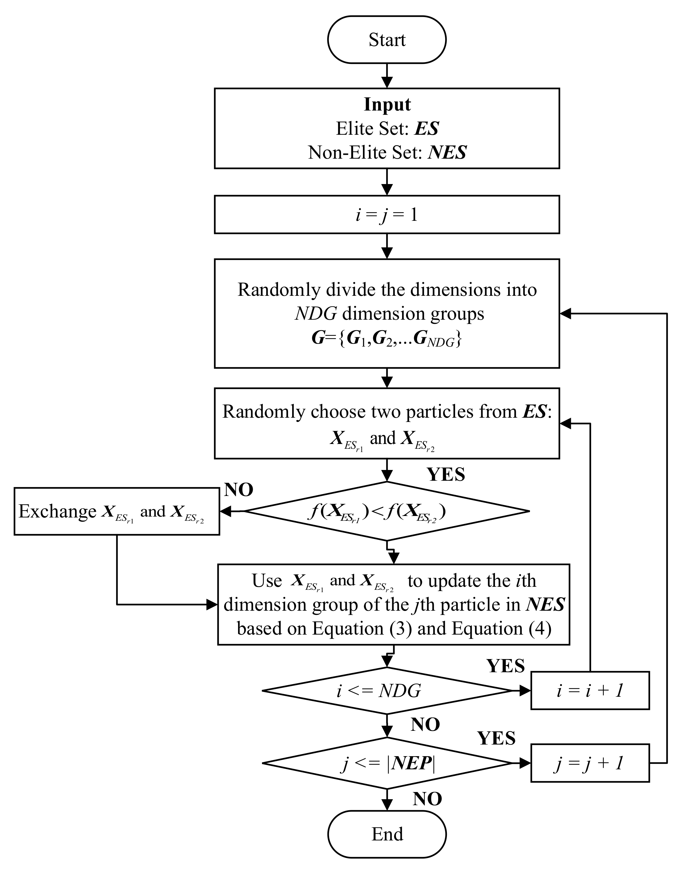
3. Dimension Group-Based Comprehensive Elite Learning Swarm Optimizer
3.1. Dimension Group-Based Comprehensive Elite Learning
- (1)
- As previously mentioned, for each non-elite particle, the dimensions are randomly shuffled. As a result, the partition of dimension groups is different for different non-elite particles.
- (2)
- For each dimension group , two different elite particles and are first randomly selected from ES. Then, the better one between these two elites (suppose it is ) acts as the first exemplar in Equation (4), while the worse one (suppose it is ) acts as the second exemplar to guide the update of the dimension group of the non-elite particle.
- (3)
- The two elite particles guiding the update of each dimension group are both randomly selected. Therefore, they are likely to be different for different dimension groups.
- (1)
- Instead of using historical evolutionary information, such as the historically global best position (gbest), the personal best positions (pbest), and the neighborhood best position (nbest), in traditional PSOs [18,47], the devised DGCEL employs the elite particles in the current swarm to direct the learning of the non-elite particles. In contrast to the historical information, which may remain unchanged for many generations, particles in the swarm are usually updated generation by generation. Therefore, in the proposed DGCEL, the selected two guiding exemplars are not only likely different for different particles but also probably different for the same particle in different generations. This is very beneficial for the promotion of swarm diversity.
- (2)
- Instead of updating each particle with the same exemplars for all dimensions in most existing large-scale PSOs [5,24,25,26,30], the proposed DGCEL updates non-elite particles at the dimension group level. Therefore, for different dimension groups, the two guiding exemplars are likely different. In this way, not only could one non-elite particle learn from multiple different elite ones, but also the useful genes hidden in different elites could be incorporated to direct the evolution of the swarm. As a result, not only the learning diversity of particles could be improved, but also the learning efficiency of particles could be promoted.
- (3)
- In DGCEL, each dimension group of a non-elite particle is guided by two randomly selected elite particles in ES. With the guidance of multiple elites, each non-elite particle is expected to approach promising areas quickly. In addition, since the elite particles in ES are not updated and directly enter the next generation, the useful evolutionary information in the current swarm is protected from being destroyed by uncertain updates. Therefore, the elites in ES become better and better as the evolution iterates, and at last, it is expected that these elites converge to the optimal areas.
Remark
- (1)
- In contrast to the three low-dimensional PSOs [46,47,48], the proposed DGCELSO uses the elite particles in the swarm to comprehensively guide the learning of the non-elite particles at the dimension group level. First, the three low-dimensional PSOs all use the personal best positions (pbests) of particles to construct only one guiding exemplar for each updated particle, whereas DGCELSO leverages the elite particles in the current swarm to construct two different guiding exemplars for each non-elite particle. Second, the three low-dimensional PSOs construct the guiding exemplar dimension by dimension. Nevertheless, DGCELSO constructs the two guiding exemplars group by group. With these two differences, DGCELSO is expected to construct more promising guiding exemplars for the updated particles, and thus the learning effectiveness and efficiency of particles could be largely promoted to explore the large-scale solution space.
- (2)
- In contrast to the large-scale PSO, namely SPLSO [30], DGCELSO uses two different elite particles to direct the update of each dimension group of each non-elite particle. First, the partition of the swarm in DGCELSO is very different from the one in SPLSO. In DGCELSO, the swarm is divided into two exclusive sets according to the fitness of particles, with the best es particles entering ES and the rest entering NES. However, in SPLSO, particles in the swarm are paired together and each paired two particles compete with each other, with the winner entering the relatively good set and the loser entering the relatively poor set. Second, for each non-elite particle, DGCELSO adopts two random elites in ES to guide the update of each dimension group, whereas in SPLSO, each dimension group of a loser is updated by only one random relatively good particle with the other exemplar being the mean position of the relatively good set, which is shared by all updated particles. Therefore, it is expected that the learning effectiveness and efficiency of particles in DGCELSO are higher than in SPLSO. Hence, DGCELSO is expected to explore and exploit the large-scale solution space more appropriately than SPLSO.
3.2. Adaptive Strategies for Control Parameters
3.2.1. Dynamic Adjustment for tp
3.2.2. Dynamic Adjustment for NDG
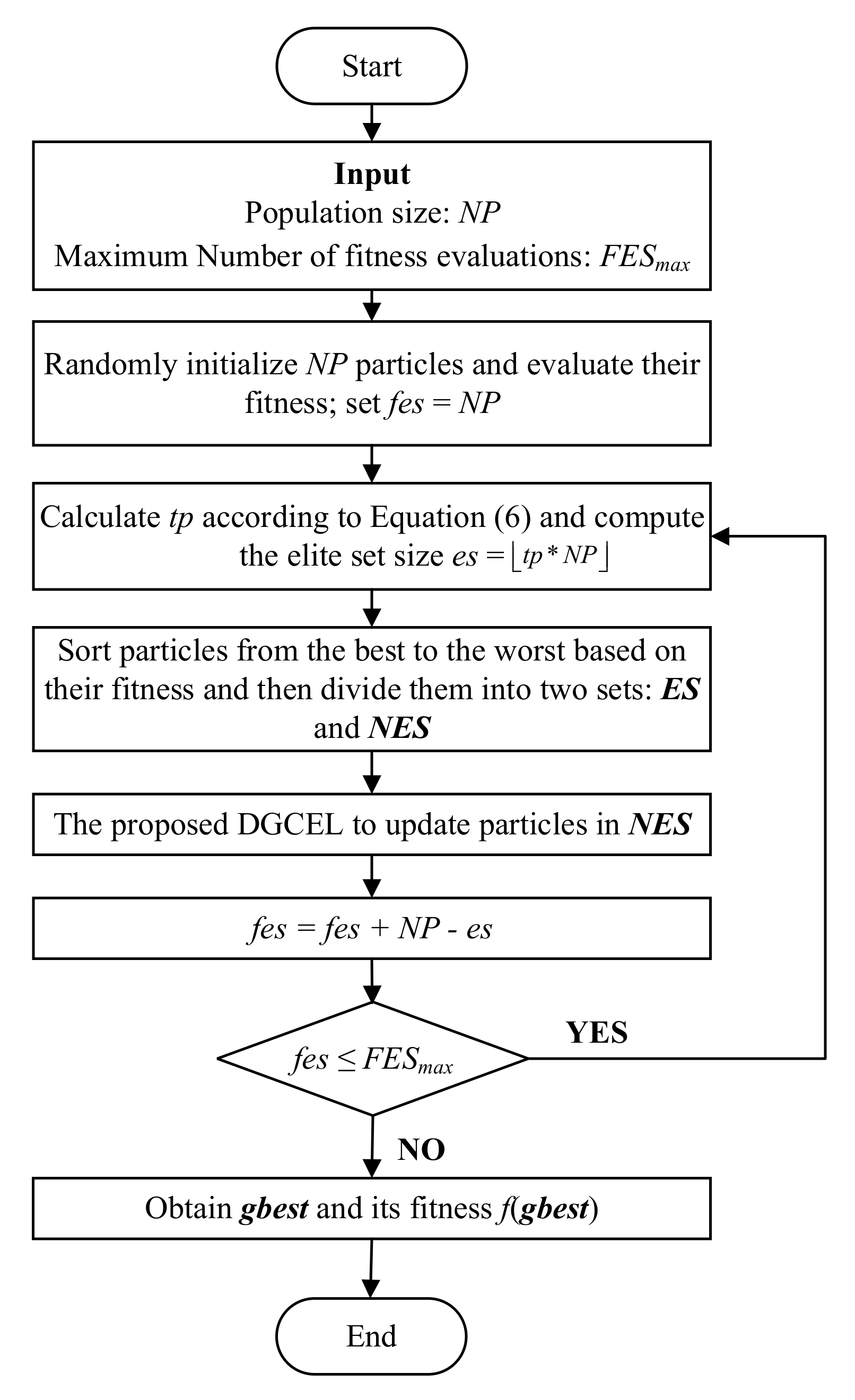
3.3. Overall Procedure of DGCELSO
| Algorithm 1: The Pseudocode of DGCELSO. | |
| Input: | Population size NP, Maximum number of fitness evaluations FESmax, Control parameter ; |
| 1: | Initialize NP particles randomly and calculate their fitness; fes = NP; |
| 2: | While (fes ≤ FESmax) do |
| 3: | Calculate tp according to Equation (6) and obtain the elite set size es = ; |
| 4: | Sort particles based on their fitness and divide them into two sets, namely ES and NES; |
| 5: | For each non-elite particle in NES do |
| 6: | Generate based on Equation (7); |
| 7: | Random shuffle the dimensions and then split the dimensions into groups; |
| 8: | For each dimension group do |
| 9: | Randomly select two different elite particles from ES: ; |
| 10: | If (f() < f()) then |
| 11: | Swap ESr1 and ESr2; |
| 12: | End If |
| 13: | Update the dimension group of according to Equations (3) and (4); |
| 14: | End For |
| 15: | Calculate the fitness of the updated , and fes ++; |
| 16: | End For |
| 17: | End While |
| 18: | Obtain the best solution in the swarm gbest and its fitness f(gbest) |
| Output: f(gbest) and gbest | |
4. Experimental Section
4.1. Parameter Setting
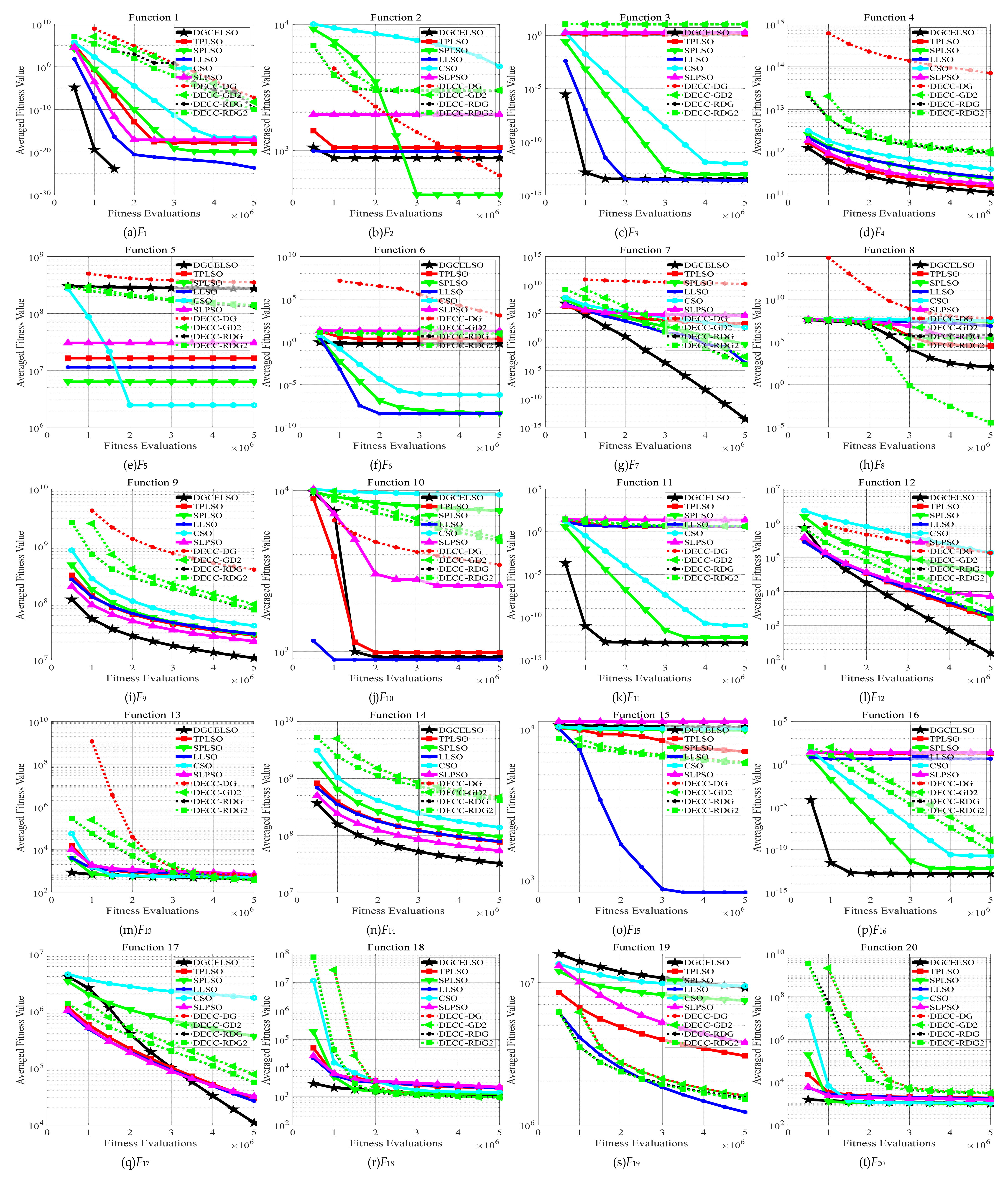
4.2. Comparisons with State-of-the-Art Methods
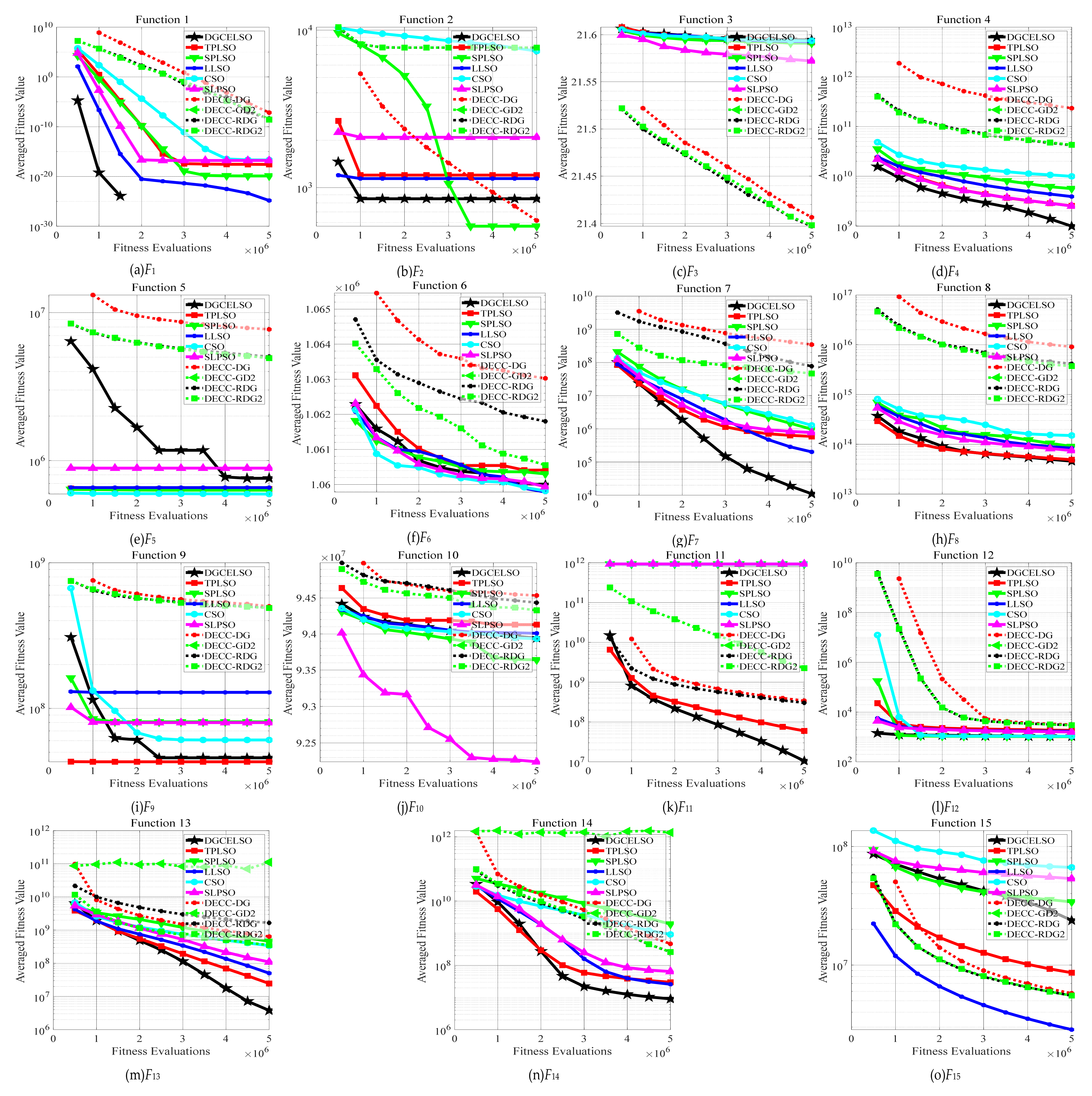
4.3. Deep Investigation on DGCELSO
4.3.1. Effectiveness of the Proposed DGCEL
4.3.2. Effectiveness of the Proposed Dynamic Adjustment Schemes for Parameters
5. Conclusions
Author Contributions
Funding
Institutional Review Board Statement
Informed Consent Statement
Data Availability Statement
Conflicts of Interest
References
- Jia, Y.H.; Mei, Y.; Zhang, M. A Two-Stage Swarm Optimizer with Local Search for Water Distribution Network Optimization. IEEE Trans. Cybern. 2021. [Google Scholar] [CrossRef]
- Cao, K.; Cui, Y.; Liu, Z.; Tan, W.; Weng, J. Edge Intelligent Joint Optimization for Lifetime and Latency in Large-Scale Cyber-Physical Systems. IEEE Internet Things J. 2021. [Google Scholar] [CrossRef]
- Chen, W.N.; Tan, D.Z.; Yang, Q.; Gu, T.; Zhang, J. Ant Colony Optimization for the Control of Pollutant Spreading on Social Networks. IEEE Trans. Cybern. 2020, 50, 4053–4065. [Google Scholar] [CrossRef]
- Zuo, T.; Zhang, Y.; Meng, K.; Tong, Z.; Dong, Z.Y.; Fu, Y. A Two-Layer Hybrid Optimization Approach for Large-Scale Offshore Wind Farm Collector System Planning. IEEE Trans. Ind. Inform. 2021, 17, 7433–7444. [Google Scholar] [CrossRef]
- Yang, Q.; Chen, W.N.; Gu, T.; Jin, H.; Mao, W.; Zhang, J. An Adaptive Stochastic Dominant Learning Swarm Optimizer for High-Dimensional Optimization. IEEE Trans. Cybern. 2020, 52, 1960–1976. [Google Scholar] [CrossRef]
- Omidvar, M.N.; Li, X.; Mei, Y.; Yao, X. Cooperative Co-Evolution with Differential Grouping for Large Scale Optimization. IEEE Trans. Evol. Comput. 2014, 18, 378–393. [Google Scholar] [CrossRef] [Green Version]
- Tang, K.; Li, X.; Suganthan, P.; Yang, Z.; Weise, T. Benchmark Functions for the CEC 2010 Special Session and Competition on Large-Scale Global Optimization; Nature Inspired Computation and Applications Laboratory, University of Science and Technology of China: Hefei, China, 2009. [Google Scholar]
- Li, X.; Tang, K.; Omidvar, M.N.; Yang, Z.; Qin, K.; China, H. Benchmark Functions for the CEC 2013 Special Session and Competition on Large-Scale Global Optimization; Technical Report; Evolutionary Computation and Machine Learning Group, RMIT University: Melbourne, Australia, 2013. [Google Scholar]
- Yang, Q.; Li, Y.; Gao, X.-D.; Ma, Y.-Y.; Lu, Z.-Y.; Jeon, S.-W.; Zhang, J. An Adaptive Covariance Scaling Estimation of Distribution Algorithm. Mathematics 2021, 9, 3207. [Google Scholar] [CrossRef]
- Yang, Q.; Chen, W.N.; Gu, T.; Zhang, H.; Yuan, H.; Kwong, S.; Zhang, J. A Distributed Swarm Optimizer with Adaptive Communication for Large-Scale Optimization. IEEE Trans. Cybern. 2020, 50, 3393–3408. [Google Scholar] [CrossRef]
- Omidvar, M.N.; Li, X.; Yao, X. A Review of Population-Based Metaheuristics for Large-Scale Black-Box Global Optimization: Part A. IEEE Trans. Evol. Comput. 2021. in press. Available online: https://ieeexplore.ieee.org/document/9627116 (accessed on 1 January 2022).
- Omidvar, M.N.; Li, X.; Yao, X. A Review of Population-Based Metaheuristics for Large-Scale Black-Box Global Optimization: Part B. IEEE Trans. Evol. Comput. 2021. in press. Available online: https://ieeexplore.ieee.org/document/9627138 (accessed on 1 January 2022).
- Yang, Q.; Xie, H.; Chen, W.; Zhang, J. Multiple Parents Guided Differential Evolution for Large Scale Optimization. In Proceedings of the IEEE Congress on Evolutionary Computation, Vancouver, BC, Canada, 24–29 July 2016; pp. 3549–3556. [Google Scholar]
- Yang, Q.; Chen, W.N.; Li, Y.; Chen, C.L.P.; Xu, X.M.; Zhang, J. Multimodal Estimation of Distribution Algorithms. IEEE Trans. Cybern. 2017, 47, 636–650. [Google Scholar] [CrossRef] [Green Version]
- Eberhart, R.; Kennedy, J. A New Optimizer Using Particle Swarm Theory. In Proceedings of the International Symposium on Micro Machine and Human Science, Nagoya, Japan, 4–6 October 1995; pp. 39–43. [Google Scholar]
- Shi, Y.; Eberhart, R. A Modified Particle Swarm Optimizer. In Proceedings of the IEEE International Conference on Evolutionary Computation Proceedings: IEEE World Congress on Computational Intelligence, Anchorage, AK, USA, 4–9 May 1998; pp. 69–73. [Google Scholar]
- Tang, J.; Liu, G.; Pan, Q. A Review on Representative Swarm Intelligence Algorithms for Solving Optimization Problems: Applications and Trends. IEEE/CAA J. Autom. Sin. 2021, 8, 1627–1643. [Google Scholar] [CrossRef]
- Ren, Z.; Zhang, A.; Wen, C.; Feng, Z. A Scatter Learning Particle Swarm Optimization Algorithm for Multimodal Problems. IEEE Trans. Cybern. 2014, 44, 1127–1140. [Google Scholar] [CrossRef]
- Zhang, J.; Lu, Y.; Che, L.; Zhou, M. Moving-Distance-Minimized PSO for Mobile Robot Swarm. IEEE Trans. Cybern. 2021. [Google Scholar] [CrossRef]
- Villalón, C.L.C.; Dorigo, M.; Stützle, T. PSO-X: A Component-Based Framework for the Automatic Design of Particle Swarm Optimization Algorithms. IEEE Trans. Evol. Comput. 2021. [Google Scholar] [CrossRef]
- Ding, W.; Lin, C.T.; Cao, Z. Deep Neuro-Cognitive Co-Evolution for Fuzzy Attribute Reduction by Quantum Leaping PSO with Nearest-Neighbor Memeplexes. IEEE Trans. Cybern. 2019, 49, 2744–2757. [Google Scholar] [CrossRef]
- Yang, Q.; Hua, L.; Gao, X.; Xu, D.; Lu, Z.; Jeon, S.-W.; Zhang, J. Stochastic Cognitive Dominance Leading Particle Swarm Optimization for Multimodal Problems. Mathematics 2022, 10, 761. [Google Scholar] [CrossRef]
- Bonavolontà, F.; Noia, L.P.D.; Liccardo, A.; Tessitore, S.; Lauria, D. A PSO-MMA Method for the Parameters Estimation of Interarea Oscillations in Electrical Grids. IEEE Trans. Instrum. Meas. 2020, 69, 8853–8865. [Google Scholar] [CrossRef]
- Lan, R.; Zhu, Y.; Lu, H.; Liu, Z.; Luo, X. A Two-Phase Learning-Based Swarm Optimizer for Large-Scale Optimization. IEEE Trans. Cybern. 2020, 51, 6284–6293. [Google Scholar] [CrossRef]
- Yang, Q.; Chen, W.; Deng, J.D.; Li, Y.; Gu, T.; Zhang, J. A Level-Based Learning Swarm Optimizer for Large-Scale Optimization. IEEE Trans. Evol. Comput. 2018, 22, 578–594. [Google Scholar] [CrossRef]
- Cheng, R.; Jin, Y. A Competitive Swarm Optimizer for Large Scale Optimization. IEEE Trans. Cybern. 2015, 45, 191–204. [Google Scholar] [CrossRef]
- Mahdavi, S.; Shiri, M.E.; Rahnamayan, S. Metaheuristics in Large-Scale Global Continues Optimization: A Survey. Inf. Sci. 2015, 295, 407–428. [Google Scholar] [CrossRef]
- Ma, X.; Li, X.; Zhang, Q.; Tang, K.; Liang, Z.; Xie, W.; Zhu, Z. A Survey on Cooperative Co-Evolutionary Algorithms. IEEE Trans. Evol. Comput. 2018, 23, 421–441. [Google Scholar] [CrossRef]
- Li, X.; Yao, X. Cooperatively Coevolving Particle Swarms for Large Scale Optimization. IEEE Trans. Evol. Comput. 2011, 16, 210–224. [Google Scholar]
- Yang, Q.; Chen, W.; Gu, T.; Zhang, H.; Deng, J.D.; Li, Y.; Zhang, J. Segment-Based Predominant Learning Swarm Optimizer for Large-Scale Optimization. IEEE Trans. Cybern. 2017, 47, 2896–2910. [Google Scholar] [CrossRef] [Green Version]
- Xie, H.Y.; Yang, Q.; Hu, X.M.; Chen, W.N. Cross-Generation Elites Guided Particle Swarm Optimization for Large Scale Optimization. In Proceedings of the IEEE Symposium Series on Computational Intelligence, Athens, Greece, 6–9 December 2016; pp. 1–8. [Google Scholar]
- Song, G.W.; Yang, Q.; Gao, X.D.; Ma, Y.Y.; Lu, Z.Y.; Zhang, J. An Adaptive Level-Based Learning Swarm Optimizer for Large-Scale Optimization. In Proceedings of the IEEE International Conference on Systems, Man, and Cybernetics, Melbourne, Australia, 17–20 October 2021; pp. 152–159. [Google Scholar]
- Potter, M.A.; De Jong, K.A. A Cooperative Co-Evolutionary Approach to Function Optimization. In Proceedings of the International Conference on Parallel Problem Solving from Nature, Berlin, Germany, 22–26 September 1994; pp. 249–257. [Google Scholar]
- Yang, Q.; Chen, W.N.; Zhang, J. Evolution Consistency Based Decomposition for Cooperative Coevolution. IEEE Access 2018, 6, 51084–51097. [Google Scholar] [CrossRef]
- Omidvar, M.N.; Yang, M.; Mei, Y.; Li, X.; Yao, X. DG2: A Faster and More Accurate Differential Grouping for Large-Scale Black-Box Optimization. IEEE Trans. Evol. Comput. 2017, 21, 929–942. [Google Scholar] [CrossRef] [Green Version]
- Sun, Y.; Kirley, M.; Halgamuge, S.K. Extended Differential Grouping for Large Scale Global Optimization with Direct and Indirect Variable Interactions. In Proceedings of the Annual Conference on Genetic and Evolutionary Computation, Madrid, Spain, 11–15 July 2015; pp. 313–320. [Google Scholar]
- Sun, Y.; Kirley, M.; Halgamuge, S.K. A Recursive Decomposition Method for Large Scale Continuous Optimization. IEEE Trans. Evol. Comput. 2017, 22, 647–661. [Google Scholar] [CrossRef]
- Song, A.; Chen, W.N.; Gong, Y.J.; Luo, X.; Zhang, J. A Divide-and-Conquer Evolutionary Algorithm for Large-Scale Virtual Network Embedding. IEEE Trans. Evol. Comput. 2020, 24, 566–580. [Google Scholar] [CrossRef]
- Deng, H.; Peng, L.; Zhang, H.; Yang, B.; Chen, Z. Ranking-Based Biased Learning Swarm Optimizer for Large-Scale Optimization. Inf. Sci. 2019, 493, 120–137. [Google Scholar] [CrossRef]
- Wang, H.; Liang, M.; Sun, C.; Zhang, G.; Xie, L. Multiple-Strategy Learning Particle Swarm Optimization for Large-Scale Optimization Problems. Complex Intell. Syst. 2021, 7, 1–16. [Google Scholar] [CrossRef]
- Jian, J.R.; Chen, Z.G.; Zhan, Z.H.; Zhang, J. Region Encoding Helps Evolutionary Computation Evolve Faster: A New Solution Encoding Scheme in Particle Swarm for Large-Scale Optimization. IEEE Trans. Evol. Comput. 2021, 25, 779–793. [Google Scholar] [CrossRef]
- Kampourakis, K. Understanding Evolution; Cambridge University Press: Cambridge, UK, 2014. [Google Scholar]
- Ju, X.; Liu, F. Wind Farm Layout Optimization Using Self-Informed Genetic Algorithm with Information Guided Exploitation. Appl. Energy 2019, 248, 429–445. [Google Scholar] [CrossRef]
- Ju, X.; Liu, F.; Wang, L.; Lee, W.-J. Wind Farm Layout Optimization Based on Support Vector Regression Guided Genetic Algorithm with Consideration of Participation among Landowners. Energy Convers. Manag. 2019, 196, 1267–1281. [Google Scholar] [CrossRef]
- Xia, X.; Gui, L.; Yu, F.; Wu, H.; Wei, B.; Zhang, Y.L.; Zhan, Z.H. Triple Archives Particle Swarm Optimization. IEEE Trans. Cybern. 2020, 50, 4862–4875. [Google Scholar] [CrossRef]
- Liang, J.J.; Qin, A.K.; Suganthan, P.N.; Baskar, S. Comprehensive Learning Particle Swarm Optimizer for Global Optimization of Multimodal Functions. IEEE Trans. Evol. Comput. 2006, 10, 281–295. [Google Scholar] [CrossRef]
- Gong, Y.; Li, J.; Zhou, Y.; Li, Y.; Chung, H.S.; Shi, Y.; Zhang, J. Genetic Learning Particle Swarm Optimization. IEEE Trans. Cybern. 2016, 46, 2277–2290. [Google Scholar] [CrossRef] [Green Version]
- Zhan, Z.; Zhang, J.; Li, Y.; Shi, Y. Orthogonal Learning Particle Swarm Optimization. IEEE Trans. Evol. Comput. 2011, 15, 832–847. [Google Scholar] [CrossRef] [Green Version]
- Van den Bergh, F.; Engelbrecht, A.P. A Cooperative Approach to Particle Swarm Optimization. IEEE Trans. Evol. Comput. 2004, 8, 225–239. [Google Scholar] [CrossRef]
- Mei, Y.; Omidvar, M.N.; Li, X.; Yao, X. A Competitive Divide-and-Conquer Algorithm for Unconstrained Large-Scale Black-Box Optimization. ACM Trans. Math. Softw. 2016, 42, 1–24. [Google Scholar] [CrossRef]
- Yang, M.; Zhou, A.; Li, C.; Yao, X. An Efficient Recursive Differential Grouping for Large-Scale Continuous Problems. IEEE Trans. Evol. Comput. 2021, 25, 159–171. [Google Scholar] [CrossRef]
- Sun, Y.; Omidvar, M.N.; Kirley, M.; Li, X. Adaptive Threshold Parameter Estimation with Recursive Differential Grouping for Problem Decomposition. In Proceedings of the Genetic and Evolutionary Computation Conference, Kyoto, Japan, 15–19 July 2018. [Google Scholar]
- Ma, X.; Huang, Z.; Li, X.; Wang, L.; Qi, Y.; Zhu, Z. Merged Differential Grouping for Large-scale Global Optimization. IEEE Trans. Evol. Comput. 2022, in press. [Google Scholar] [CrossRef]
- Liu, H.; Wang, Y.; Fan, N. A Hybrid Deep Grouping Algorithm for Large Scale Global Optimization. IEEE Trans. Evol. Comput. 2020, 24, 1112–1124. [Google Scholar] [CrossRef]
- Zhang, X.Y.; Gong, Y.J.; Lin, Y.; Zhang, J.; Kwong, S.; Zhang, J. Dynamic Cooperative Coevolution for Large Scale Optimization. IEEE Trans. Evol. Comput. 2019, 23, 935–948. [Google Scholar] [CrossRef]
- Neshat, M.; Mirjalili, S.; Sergiienko, N.Y.; Esmaeilzadeh, S.; Amini, E.; Heydari, A.; Garcia, D.A. Layout Optimisation of Offshore Wave Energy Converters Using a Novel Multi-swarm Cooperative Algorithm with Backtracking Strategy: A Case Study from Coasts of Australia. Energy 2022, 239, 122463. [Google Scholar] [CrossRef]
- Pan, Q.K.; Gao, L.; Wang, L. An Effective Cooperative Co-Evolutionary Algorithm for Distributed Flowshop Group Scheduling Problems. IEEE Trans. Cybern. 2020. [Google Scholar] [CrossRef]
- Neshat, M.; Alexander, B.; Wagner, M. A Hybrid Cooperative Co-Evolution Algorithm Framework for Optimising Power Take off and Placements of Wave Energy Converters. Inf. Sci. 2020, 534, 218–244. [Google Scholar] [CrossRef]
- Liang, M.; Wang, W.; Dong, C.; Zhao, D. A Cooperative Coevolutionary Optimization Design of Urban Transit Network and Operating Frequencies. Expert Syst. Appl. 2020, 160, 113736. [Google Scholar] [CrossRef]
- Zhao, S.-Z.; Liang, J.J.; Suganthan, P.N.; Tasgetiren, M.F. Dynamic Multi-Swarm Particle Swarm Optimizer with Local Search for Large Scale Global Optimization. In Proceedings of the IEEE Congress on Evolutionary Computation, Hong Kong, China, 1–6 June 2008; pp. 3845–3852. [Google Scholar]
- Cheng, R. A Social Learning Particle Swarm Optimization Algorithm for Scalable Optimization. Inf. Sci. 2015, 291, 43–60. [Google Scholar] [CrossRef]
- Mohapatra, P.; Das, K.N.; Roy, S. A Modified Competitive Swarm Optimizer for Large Scale Optimization Problems. Appl. Soft Comput. 2017, 59, 340–362. [Google Scholar] [CrossRef]
- Li, D.; Guo, W.; Lerch, A.; Li, Y.; Wang, L.; Wu, Q. An Adaptive Particle Swarm Optimizer with Decoupled Exploration and Exploitation for Large Scale Optimization. Swarm Evol. Comput. 2021, 60, 100789. [Google Scholar] [CrossRef]
- Lan, R.; Zhang, L.; Tang, Z.; Liu, Z.; Luo, X. A Hierarchical Sorting Swarm Optimizer for Large-Scale Optimization. IEEE Access 2019, 7, 40625–40635. [Google Scholar] [CrossRef]
- Kong, F.; Jiang, J.; Huang, Y. An Adaptive Multi-Swarm Competition Particle Swarm Optimizer for Large-Scale Optimization. Mathematics 2019, 7, 521. [Google Scholar] [CrossRef] [Green Version]
- Huang, H.; Lv, L.; Ye, S.; Hao, Z. Particle Swarm Optimization with Convergence Speed Controller for Large-Scale Numerical Optimization. Soft Comput. 2019, 23, 4421–4437. [Google Scholar] [CrossRef]
- LaTorre, A.; Muelas, S.; Peña, J.-M. A Comprehensive Comparison of Large Scale Global Optimizers. Inf. Sci. 2015, 316, 517–549. [Google Scholar] [CrossRef]


| F | NP = 100 | NP = 200 | ||||||||||||||||
| ϕ = 0.1 | ϕ = 0.2 | ϕ = 0.3 | ϕ = 0.4 | ϕ = 0.5 | ϕ = 0.6 | ϕ = 0.7 | ϕ = 0.8 | ϕ = 0.9 | ϕ = 0.1 | ϕ = 0.2 | ϕ = 0.3 | ϕ = 0.4 | ϕ = 0.5 | ϕ = 0.6 | ϕ = 0.7 | ϕ = 0.8 | ϕ = 0.9 | |
| F1 | 3.31 × 10² | 5.18 × 10⁷ | 8.23 × 10⁷ | 1.34 × 10⁷ | 1.12 × 10³ | 2.92 × 10⁻²³ | 9.51 × 10⁻²⁰ | 5.27 × 10⁵ | 1.01 × 10⁸ | 5.12 × 10⁻²⁶ | 6.22 × 10⁻²⁹ | 5.73 × 10⁻²⁷ | 0.00 × 100 | 1.10 × 10⁻²⁶ | 2.11 × 10⁻²² | 9.04 × 10² | 5.08 × 10⁷ | 1.22 × 10⁹ |
| F2 | 2.93 × 10³ | 3.58 × 10³ | 3.64 × 10³ | 3.22 × 10³ | 2.50 × 10³ | 1.62 × 10³ | 1.12 × 10³ | 9.12 × 10³ | 1.13 × 10⁴ | 1.16 × 10³ | 1.61 × 10³ | 1.69 × 10³ | 1.40 × 10³ | 8.84 × 10² | 2.95 × 10³ | 1.07 × 10⁴ | 1.14 × 10⁴ | 1.19 × 10⁴ |
| F3 | 5.74 × 100 | 1.13 × 101 | 1.14 × 101 | 8.23 × 100 | 3.24 × 100 | 2.18 × 10⁻¹ | 6.43 × 10⁻¹⁴ | 3.89 × 10⁻¹ | 1.36 × 101 | 3.47 × 10⁻¹⁴ | 2.90 × 10⁻² | 1.19 × 10⁻¹ | 3.42 × 10⁻¹⁴ | 3.81 × 10⁻¹⁴ | 4.88 × 10⁻¹⁴ | 3.63 × 10⁻¹ | 1.27 × 101 | 1.71 × 101 |
| F4 | 4.77 × 10¹¹ | 5.57 × 10¹² | 5.93 × 10¹² | 2.88 × 10¹² | 1.66 × 10¹¹ | 1.14 × 10¹¹ | 1.53 × 10¹¹ | 2.90 × 10¹¹ | 7.08 × 10¹¹ | 1.74 × 10¹¹ | 1.96 × 10¹¹ | 4.21 × 10¹¹ | 1.28 × 10¹¹ | 1.25 × 10¹¹ | 1.67 × 10¹¹ | 2.48 × 10¹¹ | 6.04 × 10¹¹ | 2.14 × 10¹³ |
| F5 | 2.96 × 10⁷ | 3.16 × 10⁷ | 3.01 × 10⁷ | 3.54 × 10⁷ | 1.30 × 10⁸ | 2.75 × 10⁸ | 2.86 × 10⁸ | 2.96 × 10⁸ | 3.05 × 10⁸ | 2.81 × 10⁸ | 2.36 × 10⁸ | 2.24 × 10⁸ | 2.55 × 10⁸ | 2.77 × 10⁸ | 2.84 × 10⁸ | 2.91 × 10⁸ | 3.04 × 10⁸ | 3.09 × 10⁸ |
| F6 | 1.99 × 101 | 2.02 × 101 | 2.02 × 101 | 2.01 × 101 | 1.99 × 101 | 2.01 × 101 | 2.15 × 101 | 2.15 × 101 | 2.03 × 101 | 1.94 × 101 | 1.97 × 101 | 1.97 × 101 | 1.98 × 101 | 1.96 × 101 | 4.00 × 10⁻⁹ | 3.82 × 10⁻¹ | 1.34 × 101 | 1.78 × 101 |
| F7 | 2.94 × 10⁶ | 9.82 × 10⁸ | 1.28 × 10⁹ | 3.37 × 10⁸ | 7.90 × 10⁵ | 7.40 × 10⁵ | 1.17 × 10⁵ | 8.40 × 10⁴ | 7.80 × 10⁵ | 3.34 × 10⁻⁶ | 3.70 × 10⁴ | 1.75 × 10⁶ | 1.40 × 10³ | 8.73 × 10⁻⁶ | 3.14 × 10⁻¹ | 2.51 × 10⁴ | 5.02 × 10⁵ | 1.76 × 10⁷ |
| F8 | 3.39 × 10⁷ | 4.89 × 10⁷ | 4.72 × 10⁷ | 4.42 × 10⁷ | 1.67 × 10⁵ | 6.68 × 10⁴ | 1.58 × 10⁷ | 4.17 × 10⁷ | 4.89 × 10⁷ | 3.33 × 10⁵ | 5.47 × 10⁶ | 2.47 × 10⁷ | 1.86 × 10³ | 3.95 × 10³ | 1.73 × 10⁷ | 3.97 × 10⁷ | 4.52 × 10⁷ | 4.62 × 10⁷ |
| F9 | 8.72 × 10⁷ | 1.03 × 10⁹ | 1.17 × 10⁹ | 6.34 × 10⁸ | 2.80 × 10⁷ | 1.75 × 10⁷ | 4.08 × 10⁷ | 4.70 × 10⁸ | 1.36 × 10¹⁰ | 1.97 × 10⁷ | 3.44 × 10⁷ | 6.48 × 10⁷ | 1.98 × 10⁷ | 1.47 × 10⁷ | 4.03 × 10⁷ | 3.65 × 10⁹ | 2.29 × 10¹⁰ | 4.11 × 10¹⁰ |
| F10 | 3.14 × 10³ | 3.85 × 10³ | 3.97 × 10³ | 3.43 × 10³ | 2.65 × 10³ | 1.69 × 10³ | 2.66 × 10³ | 1.09 × 10⁴ | 1.16 × 10⁴ | 1.20 × 10³ | 1.76 × 10³ | 1.82 × 10³ | 1.48 × 10³ | 9.59 × 10² | 1.01 × 10⁴ | 1.08 × 10⁴ | 1.14 × 10⁴ | 1.20 × 10⁴ |
| F11 | 7.08 × 101 | 9.71 × 101 | 9.38 × 101 | 8.60 × 101 | 5.22 × 101 | 3.03 × 101 | 2.47 × 101 | 2.53 × 101 | 6.32 × 101 | 1.57 × 101 | 2.00 × 101 | 2.03 × 101 | 2.00 × 101 | 1.09 × 101 | 1.85 × 10⁻¹³ | 1.38 × 100 | 5.04 × 101 | 1.41 × 10² |
| F12 | 9.54 × 10⁴ | 1.03 × 10⁶ | 1.13 × 10⁶ | 6.89 × 10⁵ | 4.82 × 10³ | 8.18 × 10² | 6.14 × 10⁴ | 5.07 × 10⁶ | 6.64 × 10⁶ | 2.35 × 10³ | 1.71 × 10⁴ | 7.25 × 10⁴ | 1.72 × 10³ | 1.92 × 10³ | 2.36 × 10⁶ | 5.14 × 10⁶ | 6.61 × 10⁶ | 7.97 × 10⁶ |
| F13 | 5.89 × 10³ | 3.83 × 10⁶ | 4.40 × 10⁶ | 9.77 × 10⁵ | 5.29 × 10³ | 3.06 × 10³ | 2.35 × 10³ | 6.58 × 10⁴ | 1.36 × 10⁸ | 6.55 × 10² | 8.02 × 10² | 1.02 × 10³ | 5.58 × 10² | 4.97 × 10² | 5.48 × 10² | 2.96 × 10³ | 3.95 × 10⁷ | 9.38 × 10⁹ |
| F14 | 2.68 × 10⁸ | 2.11 × 10⁹ | 2.30 × 10⁹ | 1.45 × 10⁹ | 8.31 × 10⁷ | 4.56 × 10⁷ | 1.39 × 10⁸ | 3.47 × 10⁹ | 3.23 × 10¹⁰ | 5.82 × 10⁷ | 1.12 × 10⁸ | 2.20 × 10⁸ | 6.07 × 10⁷ | 4.61 × 10⁷ | 2.11 × 10⁸ | 2.02 × 10¹⁰ | 5.18 × 10¹⁰ | 7.58 × 10¹⁰ |
| F15 | 3.33 × 10³ | 4.07 × 10³ | 4.13 × 10³ | 3.53 × 10³ | 2.81 × 10³ | 1.11 × 10⁴ | 1.09 × 10⁴ | 1.12 × 10⁴ | 1.17 × 10⁴ | 1.07 × 10⁴ | 3.71 × 10³ | 3.33 × 10³ | 1.07 × 10⁴ | 1.05 × 10⁴ | 1.05 × 10⁴ | 1.08 × 10⁴ | 1.14 × 10⁴ | 1.21 × 10⁴ |
| F16 | 1.89 × 10² | 2.56 × 10² | 2.56 × 10² | 2.22 × 10² | 1.47 × 10² | 8.35 × 101 | 5.10 × 101 | 6.61 × 101 | 2.58 × 10² | 6.10 × 10⁻¹ | 1.60 × 101 | 2.71 × 101 | 6.75 × 100 | 3.42 × 10⁻² | 2.93 × 10⁻¹³ | 1.35 × 101 | 2.52 × 10² | 3.39 × 10² |
| F17 | 3.02 × 10⁵ | 1.61 × 10⁶ | 1.71 × 10⁶ | 1.27 × 10⁶ | 3.52 × 10⁴ | 1.06 × 10⁴ | 2.08 × 10⁶ | 9.92 × 10⁶ | 1.40 × 10⁷ | 4.93 × 10⁴ | 9.98 × 10⁴ | 2.77 × 10⁵ | 2.24 × 10⁴ | 1.18 × 10⁵ | 6.85 × 10⁶ | 1.08 × 10⁷ | 1.47 × 10⁷ | 1.80 × 10⁷ |
| F18 | 1.70 × 10⁴ | 7.87 × 10⁸ | 1.16 × 10⁹ | 3.75 × 10⁷ | 2.67 × 10³ | 1.71 × 10³ | 2.72 × 10³ | 6.17 × 10⁶ | 4.49 × 10¹⁰ | 1.95 × 10³ | 2.54 × 10³ | 3.90 × 10³ | 1.66 × 10³ | 1.30 × 10³ | 1.59 × 10³ | 1.71 × 10⁷ | 2.95 × 10¹⁰ | 1.40 × 10¹¹ |
| F19 | 2.34 × 10⁶ | 4.66 × 10⁶ | 4.74 × 10⁶ | 3.92 × 10⁶ | 1.72 × 10⁶ | 6.52 × 10⁶ | 1.48 × 10⁷ | 2.01 × 10⁷ | 2.49 × 10⁷ | 9.10 × 10⁶ | 2.46 × 10⁶ | 2.41 × 10⁶ | 5.98 × 10⁶ | 1.09 × 10⁷ | 1.60 × 10⁷ | 2.09 × 10⁷ | 2.58 × 10⁷ | 3.04 × 10⁷ |
| F20 | 8.41 × 10³ | 1.01 × 10⁹ | 1.39 × 10⁹ | 4.32 × 10⁷ | 2.93 × 10³ | 1.29 × 10³ | 1.25 × 10³ | 7.61 × 10⁶ | 4.93 × 10¹⁰ | 1.41 × 10³ | 2.13 × 10³ | 2.72 × 10³ | 1.51 × 10³ | 1.10 × 10³ | 1.02 × 10³ | 2.27 × 10⁷ | 3.25 × 10¹⁰ | 1.47 × 10¹¹ |
| Rank | 3.75 | 6.35 | 7.05 | 5.30 | 2.80 | 2.45 | 3.25 | 5.75 | 8.30 | 3.25 | 4.25 | 5.25 | 3.15 | 2.45 | 3.95 | 6.25 | 7.70 | 8.75 |
| F | NP = 300 | NP = 400 | ||||||||||||||||
| ϕ = 0.1 | ϕ = 0.2 | ϕ = 0.3 | ϕ = 0.4 | ϕ = 0.5 | ϕ = 0.6 | ϕ = 0.7 | ϕ = 0.8 | ϕ = 0.9 | ϕ = 0.1 | ϕ = 0.2 | ϕ = 0.3 | ϕ = 0.4 | ϕ = 0.5 | ϕ = 0.6 | ϕ = 0.7 | ϕ = 0.8 | ϕ = 0.9 | |
| F1 | 9.78 × 10⁻²⁷ | 0.00 × 100 | 0.00 × 100 | 0.00 × 100 | 0.00 × 100 | 7.97 × 10⁻¹⁰ | 5.83 × 10⁵ | 1.86 × 10⁸ | 2.23 × 10⁹ | 6.50 × 10⁻²⁴ | 0.00 × 100 | 0.00 × 100 | 0.00 × 100 | 8.36 × 10⁻²⁴ | 4.18 × 10⁻³ | 3.39 × 10⁶ | 3.30 × 10⁸ | 3.01 × 10⁹ |
| F2 | 6.93 × 10² | 1.06 × 10³ | 1.15 × 10³ | 8.88 × 10² | 5.90 × 10² | 1.04 × 10⁴ | 1.09 × 10⁴ | 1.15 × 10⁴ | 1.21 × 10⁴ | 5.75 × 10² | 8.12 × 10² | 8.78 × 10² | 6.57 × 10² | 9.82 × 10³ | 1.05 × 10⁴ | 1.10 × 10⁴ | 1.16 × 10⁴ | 1.22 × 10⁴ |
| F3 | 3.36 × 10⁻¹⁴ | 3.05 × 10⁻¹⁴ | 3.15 × 10⁻¹⁴ | 3.18 × 10⁻¹⁴ | 3.88 × 10⁻¹⁴ | 1.15 × 10⁻⁷ | 5.14 × 100 | 1.47 × 101 | 1.77 × 101 | 3.51 × 10⁻¹⁴ | 2.99 × 10⁻¹⁴ | 2.98 × 10⁻¹⁴ | 3.15 × 10⁻¹⁴ | 3.98 × 10⁻¹⁴ | 3.29 × 10⁻⁴ | 7.64 × 100 | 1.54 × 101 | 1.79 × 101 |
| F4 | 2.22 × 10¹¹ | 2.13 × 10¹¹ | 2.00 × 10¹¹ | 1.60 × 10¹¹ | 1.57 × 10¹¹ | 2.06 × 10¹¹ | 3.80 × 10¹¹ | 1.31 × 10¹² | 6.16 × 10¹³ | 2.88 × 10¹¹ | 2.60 × 10¹¹ | 2.27 × 10¹¹ | 1.96 × 10¹¹ | 1.82 × 10¹¹ | 2.48 × 10¹¹ | 5.19 × 10¹¹ | 3.12 × 10¹² | 1.09 × 10¹⁴ |
| F5 | 2.83 × 10⁸ | 2.81 × 10⁸ | 2.76 × 10⁸ | 2.80 × 10⁸ | 2.82 × 10⁸ | 2.86 × 10⁸ | 2.93 × 10⁸ | 3.02 × 10⁸ | 3.18 × 10⁸ | 2.82 × 10⁸ | 2.82 × 10⁸ | 2.81 × 10⁸ | 2.78 × 10⁸ | 2.83 × 10⁸ | 2.89 × 10⁸ | 2.94 × 10⁸ | 3.06 × 10⁸ | 3.16 × 10⁸ |
| F6 | 4.00 × 10⁻⁹ | 6.18 × 100 | 1.86 × 101 | 4.00 × 10⁻⁹ | 4.00 × 10⁻⁹ | 2.08 × 10⁻⁷ | 5.36 × 100 | 1.54 × 101 | 1.84 × 101 | 4.00 × 10⁻⁹ | 3.88 × 10⁻⁹ | 4.00 × 10⁻⁹ | 4.00 × 10⁻⁹ | 4.00 × 10⁻⁹ | 4.72 × 10⁻⁴ | 8.08 × 100 | 1.61 × 101 | 1.86 × 101 |
| F7 | 3.43 × 10⁻³ | 1.20 × 10⁻³ | 3.63 × 10⁻² | 2.15 × 10⁻⁵ | 2.54 × 10⁻³ | 3.60 × 10² | 1.83 × 10⁵ | 9.66 × 10⁵ | 4.68 × 10⁸ | 8.32 × 10⁻¹ | 3.50 × 10⁻² | 3.16 × 10⁻² | 7.06 × 10⁻³ | 1.03 × 100 | 7.18 × 10³ | 3.40 × 10⁵ | 5.23 × 10⁶ | 1.55 × 10⁹ |
| F8 | 1.37 × 10⁷ | 3.51 × 10⁵ | 3.72 × 10⁴ | 4.36 × 10³ | 9.82 × 10⁵ | 3.01 × 10⁷ | 4.30 × 10⁷ | 4.58 × 10⁷ | 4.65 × 10⁷ | 2.23 × 10⁷ | 1.00 × 10⁷ | 3.36 × 10⁶ | 6.67 × 10⁵ | 1.33 × 10⁷ | 3.52 × 10⁷ | 4.41 × 10⁷ | 4.61 × 10⁷ | 4.67 × 10⁷ |
| F9 | 2.47 × 10⁷ | 2.28 × 10⁷ | 2.49 × 10⁷ | 1.77 × 10⁷ | 2.14 × 10⁷ | 1.69 × 10⁸ | 1.40 × 10¹⁰ | 3.19 × 10¹⁰ | 5.08 × 10¹⁰ | 3.12 × 10⁷ | 2.42 × 10⁷ | 2.41 × 10⁷ | 2.01 × 10⁷ | 3.01 × 10⁷ | 1.36 × 10⁹ | 1.92 × 10¹⁰ | 3.70 × 10¹⁰ | 5.55 × 10¹⁰ |
| F10 | 8.49 × 10² | 1.13 × 10³ | 1.22 × 10³ | 9.23 × 10² | 9.75 × 10³ | 1.05 × 10⁴ | 1.09 × 10⁴ | 1.15 × 10⁴ | 1.22 × 10⁴ | 9.74 × 10³ | 8.59 × 10² | 9.25 × 10² | 1.11 × 10³ | 1.02 × 10⁴ | 1.05 × 10⁴ | 1.10 × 10⁴ | 1.16 × 10⁴ | 1.22 × 10⁴ |
| F11 | 1.25 × 10⁻¹³ | 2.23 × 10⁻¹ | 6.68 × 100 | 1.10 × 10⁻¹³ | 1.17 × 10⁻¹³ | 3.45 × 10⁻⁷ | 8.82 × 100 | 7.59 × 101 | 1.59 × 10² | 1.30 × 10⁻¹³ | 1.11 × 10⁻¹³ | 1.05 × 10⁻¹³ | 1.06 × 10⁻¹³ | 1.31 × 10⁻¹³ | 7.60 × 10⁻⁴ | 1.51 × 101 | 9.53 × 101 | 1.67 × 10² |
| F12 | 2.50 × 10⁴ | 4.39 × 10³ | 5.55 × 10³ | 2.55 × 10³ | 8.74 × 10⁴ | 4.13 × 10⁶ | 5.75 × 10⁶ | 7.14 × 10⁶ | 8.45 × 10⁶ | 1.71 × 10⁵ | 9.83 × 10³ | 7.41 × 10³ | 1.18 × 10⁴ | 2.03 × 10⁶ | 4.62 × 10⁶ | 6.16 × 10⁶ | 7.49 × 10⁶ | 8.77 × 10⁶ |
| F13 | 5.69 × 10² | 5.35 × 10² | 5.91 × 10² | 5.15 × 10² | 4.69 × 10² | 4.85 × 10² | 1.08 × 10⁵ | 5.63 × 10⁸ | 1.67 × 10¹⁰ | 5.31 × 10² | 5.36 × 10² | 5.46 × 10² | 4.93 × 10² | 4.50 × 10² | 4.80 × 10² | 3.72 × 10⁵ | 1.46 × 10⁹ | 2.23 × 10¹⁰ |
| F14 | 7.79 × 10⁷ | 6.96 × 10⁷ | 7.62 × 10⁷ | 5.17 × 10⁷ | 7.69 × 10⁷ | 5.73 × 10⁹ | 3.85 × 10¹⁰ | 6.50 × 10¹⁰ | 8.96 × 10¹⁰ | 1.14 × 10⁸ | 7.11 × 10⁷ | 7.20 × 10⁷ | 6.01 × 10⁷ | 1.43 × 10⁸ | 1.68 × 10¹⁰ | 4.63 × 10¹⁰ | 7.22 × 10¹⁰ | 9.64 × 10¹⁰ |
| F15 | 1.04 × 10⁴ | 1.05 × 10⁴ | 1.05 × 10⁴ | 1.04 × 10⁴ | 1.03 × 10⁴ | 1.06 × 10⁴ | 1.10 × 10⁴ | 1.16 × 10⁴ | 1.22 × 10⁴ | 1.04 × 10⁴ | 1.03 × 10⁴ | 1.04 × 10⁴ | 1.03 × 10⁴ | 1.03 × 10⁴ | 1.06 × 10⁴ | 1.11 × 10⁴ | 1.17 × 10⁴ | 1.23 × 10⁴ |
| F16 | 2.15 × 10⁻¹³ | 5.86 × 10⁻² | 9.78 × 10⁻² | 1.55 × 10⁻¹³ | 2.01 × 10⁻¹³ | 2.36 × 10⁻⁶ | 1.02 × 10² | 2.92 × 10² | 3.52 × 10² | 2.39 × 10⁻¹³ | 1.61 × 10⁻¹³ | 1.53 × 10⁻¹³ | 1.60 × 10⁻¹³ | 2.44 × 10⁻¹³ | 7.14 × 10⁻³ | 1.52 × 10² | 3.07 × 10² | 3.57 × 10² |
| F17 | 1.53 × 10⁶ | 5.71 × 10⁴ | 5.65 × 10⁴ | 6.57 × 10⁴ | 4.44 × 10⁶ | 8.75 × 10⁶ | 1.28 × 10⁷ | 1.65 × 10⁷ | 1.98 × 10⁷ | 4.81 × 10⁶ | 1.72 × 10⁵ | 1.03 × 10⁵ | 7.07 × 10⁵ | 6.20 × 10⁶ | 1.02 × 10⁷ | 1.37 × 10⁷ | 1.72 × 10⁷ | 2.06 × 10⁷ |
| F18 | 1.56 × 10³ | 1.65 × 10³ | 1.56 × 10³ | 1.31 × 10³ | 1.13 × 10³ | 1.26 × 10³ | 1.57 × 10⁹ | 5.42 × 10¹⁰ | 1.76 × 10¹¹ | 1.31 × 10³ | 1.31 × 10³ | 1.33 × 10³ | 1.25 × 10³ | 1.12 × 10³ | 3.88 × 10³ | 4.92 × 10⁹ | 6.87 × 10¹⁰ | 1.94 × 10¹¹ |
| F19 | 1.33 × 10⁷ | 8.92 × 10⁶ | 8.14 × 10⁶ | 1.02 × 10⁷ | 1.43 × 10⁷ | 1.88 × 10⁷ | 2.25 × 10⁷ | 2.75 × 10⁷ | 3.21 × 10⁷ | 1.45 × 10⁷ | 1.09 × 10⁷ | 1.02 × 10⁷ | 1.21 × 10⁷ | 1.53 × 10⁷ | 1.94 × 10⁷ | 2.47 × 10⁷ | 2.87 × 10⁷ | 3.36 × 10⁷ |
| F20 | 1.12 × 10³ | 1.32 × 10³ | 1.40 × 10³ | 1.08 × 10³ | 9.79 × 10² | 1.00 × 10³ | 1.88 × 10⁹ | 5.74 × 10¹⁰ | 1.82 × 10¹¹ | 9.89 × 10² | 1.15 × 10³ | 1.10 × 10³ | 9.85 × 10² | 9.82 × 10² | 1.72 × 10³ | 5.69 × 10⁹ | 7.40 × 10¹⁰ | 2.03 × 10¹¹ |
| Rank | 3.80 | 3.48 | 4.03 | 2.03 | 2.88 | 5.00 | 6.90 | 7.95 | 8.95 | 3.90 | 2.90 | 2.50 | 2.05 | 3.95 | 5.70 | 7.00 | 8.00 | 9.00 |
| F | NP = 500 | NP = 600 | ||||||||||||||||
| ϕ = 0.1 | ϕ = 0.2 | ϕ = 0.3 | ϕ = 0.4 | ϕ = 0.5 | ϕ = 0.6 | ϕ = 0.7 | ϕ = 0.8 | ϕ = 0.9 | ϕ = 0.1 | ϕ = 0.2 | ϕ = 0.3 | ϕ = 0.4 | ϕ = 0.5 | ϕ = 0.6 | ϕ = 0.7 | ϕ = 0.8 | ϕ = 0.9 | |
| F1 | 8.02 × 10⁻²² | 0.00 × 100 | 0.00 × 100 | 0.00 × 100 | 6.91 × 10⁻²¹ | 4.51 × 100 | 8.52 × 10⁶ | 4.72 × 10⁸ | 3.65 × 10⁹ | 2.72 × 10⁻¹⁹ | 2.86 × 10⁻²⁶ | 0.00 × 100 | 5.33 × 10⁻²⁶ | 9.43 × 10⁻¹⁶ | 1.90 × 10² | 1.57 × 10⁷ | 6.02 × 10⁸ | 4.18 × 10⁹ |
| F2 | 8.73 × 10³ | 6.81 × 10² | 7.34 × 10² | 5.74 × 10² | 1.01 × 10⁴ | 1.06 × 10⁴ | 1.11 × 10⁴ | 1.16 × 10⁴ | 1.23 × 10⁴ | 9.87 × 10³ | 6.03 × 10² | 6.59 × 10² | 4.15 × 10³ | 1.02 × 10⁴ | 1.06 × 10⁴ | 1.11 × 10⁴ | 1.17 × 10⁴ | 1.23 × 10⁴ |
| F3 | 3.92 × 10⁻¹⁴ | 2.96 × 10⁻¹⁴ | 2.90 × 10⁻¹⁴ | 3.12 × 10⁻¹⁴ | 8.55 × 10⁻¹⁴ | 1.24 × 10⁻² | 9.15 × 100 | 1.58 × 101 | 1.80 × 101 | 8.00 × 10⁻¹³ | 2.97 × 10⁻¹⁴ | 2.90 × 10⁻¹⁴ | 3.16 × 10⁻¹⁴ | 6.07 × 10⁻¹¹ | 1.06 × 10⁻¹ | 1.02 × 101 | 1.61 × 101 | 1.82 × 101 |
| F4 | 3.35 × 10¹¹ | 3.11 × 10¹¹ | 2.86 × 10¹¹ | 2.49 × 10¹¹ | 2.16 × 10¹¹ | 3.21 × 10¹¹ | 6.31 × 10¹¹ | 1.05 × 10¹³ | 1.22 × 10¹⁴ | 4.16 × 10¹¹ | 3.83 × 10¹¹ | 3.30 × 10¹¹ | 2.84 × 10¹¹ | 2.67 × 10¹¹ | 3.79 × 10¹¹ | 7.59 × 10¹¹ | 1.73 × 10¹³ | 1.39 × 10¹⁴ |
| F5 | 2.80 × 10⁸ | 2.76 × 10⁸ | 2.78 × 10⁸ | 2.77 × 10⁸ | 2.77 × 10⁸ | 2.90 × 10⁸ | 2.95 × 10⁸ | 3.06 × 10⁸ | 3.20 × 10⁸ | 2.80 × 10⁸ | 2.79 × 10⁸ | 2.76 × 10⁸ | 2.79 × 10⁸ | 2.84 × 10⁸ | 2.87 × 10⁸ | 2.99 × 10⁸ | 3.03 × 10⁸ | 3.18 × 10⁸ |
| F6 | 4.00 × 10⁻⁹ | 4.00 × 10⁻⁹ | 4.00 × 10⁻⁹ | 4.00 × 10⁻⁹ | 4.00 × 10⁻⁹ | 1.69 × 10⁻² | 9.72 × 100 | 1.66 × 101 | 1.88 × 101 | 4.09 × 10⁻⁹ | 3.88 × 10⁻⁹ | 3.88 × 10⁻⁹ | 4.00 × 10⁻⁹ | 6.07 × 10⁻⁹ | 1.45 × 10⁻¹ | 1.08 × 101 | 1.68 × 101 | 1.89 × 101 |
| F7 | 2.61 × 101 | 1.21 × 100 | 7.81 × 10⁻¹ | 4.75 × 10⁻¹ | 3.43 × 101 | 3.08 × 10⁴ | 4.80 × 10⁵ | 3.01 × 10⁷ | 2.65 × 10⁹ | 2.63 × 10² | 1.79 × 101 | 1.21 × 101 | 8.88 × 100 | 3.52 × 10² | 7.34 × 10⁴ | 6.46 × 10⁵ | 1.15 × 10⁸ | 3.95 × 10⁹ |
| F8 | 2.74 × 10⁷ | 1.73 × 10⁷ | 1.16 × 10⁷ | 9.50 × 10⁶ | 2.05 × 10⁷ | 3.79 × 10⁷ | 4.47 × 10⁷ | 4.63 × 10⁷ | 4.68 × 10⁷ | 3.08 × 10⁷ | 2.23 × 10⁷ | 1.74 × 10⁷ | 1.59 × 10⁷ | 2.52 × 10⁷ | 3.96 × 10⁷ | 4.50 × 10⁷ | 4.64 × 10⁷ | 4.69 × 10⁷ |
| F9 | 3.94 × 10⁷ | 2.71 × 10⁷ | 2.62 × 10⁷ | 2.33 × 10⁷ | 4.11 × 10⁷ | 4.17 × 10⁹ | 2.23 × 10¹⁰ | 4.01 × 10¹⁰ | 5.87 × 10¹⁰ | 4.84 × 10⁷ | 3.01 × 10⁷ | 2.85 × 10⁷ | 2.62 × 10⁷ | 5.78 × 10⁷ | 6.49 × 10⁹ | 2.49 × 10¹⁰ | 4.26 × 10¹⁰ | 6.14 × 10¹⁰ |
| F10 | 1.00 × 10⁴ | 1.35 × 10³ | 7.94 × 10² | 9.73 × 10³ | 1.02 × 10⁴ | 1.06 × 10⁴ | 1.11 × 10⁴ | 1.17 × 10⁴ | 1.23 × 10⁴ | 1.02 × 10⁴ | 9.45 × 10³ | 6.43 × 10³ | 9.99 × 10³ | 1.03 × 10⁴ | 1.06 × 10⁴ | 1.11 × 10⁴ | 1.17 × 10⁴ | 1.24 × 10⁴ |
| F11 | 1.67 × 10⁻¹³ | 1.11 × 10⁻¹³ | 1.04 × 10⁻¹³ | 1.10 × 10⁻¹³ | 5.51 × 10⁻¹³ | 2.59 × 10⁻² | 1.94 × 101 | 1.08 × 10² | 1.72 × 10² | 6.69 × 10⁻¹² | 1.12 × 10⁻¹³ | 1.05 × 10⁻¹³ | 1.13 × 10⁻¹³ | 4.00 × 10⁻¹⁰ | 1.90 × 10⁻¹ | 2.66 × 101 | 1.17 × 10² | 1.75 × 10² |
| F12 | 1.54 × 10⁶ | 2.34 × 10⁴ | 1.47 × 10⁴ | 4.12 × 10⁴ | 3.02 × 10⁶ | 4.87 × 10⁶ | 6.37 × 10⁶ | 7.75 × 10⁶ | 9.01 × 10⁶ | 2.65 × 10⁶ | 4.99 × 10⁴ | 2.82 × 10⁴ | 1.18 × 10⁵ | 3.37 × 10⁶ | 5.07 × 10⁶ | 6.50 × 10⁶ | 7.83 × 10⁶ | 9.11 × 10⁶ |
| F13 | 5.27 × 10² | 4.92 × 10² | 4.67 × 10² | 4.65 × 10² | 4.69 × 10² | 4.80 × 10² | 1.08 × 10⁶ | 2.45 × 10⁹ | 2.62 × 10¹⁰ | 4.82 × 10² | 5.44 × 10² | 5.20 × 10² | 4.56 × 10² | 4.42 × 10² | 5.63 × 10² | 3.15 × 10⁶ | 3.37 × 10⁹ | 2.90 × 10¹⁰ |
| F14 | 1.66 × 10⁸ | 8.14 × 10⁷ | 7.67 × 10⁷ | 7.21 × 10⁷ | 3.28 × 10⁸ | 2.36 × 10¹⁰ | 5.14 × 10¹⁰ | 7.78 × 10¹⁰ | 1.30 × 10¹¹ | 2.61 × 10⁸ | 9.02 × 10⁷ | 8.54 × 10⁷ | 8.71 × 10⁷ | 8.67 × 10⁸ | 2.77 × 10¹⁰ | 5.44 × 10¹⁰ | 7.81 × 10¹⁰ | 1.03 × 10¹¹ |
| F15 | 1.03 × 10⁴ | 1.03 × 10⁴ | 1.03 × 10⁴ | 1.03 × 10⁴ | 1.03 × 10⁴ | 1.07 × 10⁴ | 1.11 × 10⁴ | 1.17 × 10⁴ | 1.24 × 10⁴ | 1.03 × 10⁴ | 1.03 × 10⁴ | 1.03 × 10⁴ | 1.03 × 10⁴ | 1.03 × 10⁴ | 1.07 × 10⁴ | 1.12 × 10⁴ | 1.17 × 10⁴ | 1.24 × 10⁴ |
| F16 | 2.83 × 10⁻¹³ | 1.65 × 10⁻¹³ | 1.55 × 10⁻¹³ | 1.66 × 10⁻¹³ | 1.34 × 10⁻¹² | 2.74 × 10⁻¹ | 1.83 × 10² | 3.16 × 10² | 3.61 × 10² | 1.54 × 10⁻¹¹ | 1.74 × 10⁻¹³ | 1.58 × 10⁻¹³ | 1.80 × 10⁻¹³ | 1.18 × 10⁻⁹ | 2.41 × 100 | 2.05 × 10² | 3.22 × 10² | 3.63 × 10² |
| F17 | 5.98 × 10⁶ | 7.91 × 10⁵ | 2.80 × 10⁵ | 3.07 × 10⁶ | 7.05 × 10⁶ | 1.07 × 10⁷ | 1.43 × 10⁷ | 1.76 × 10⁷ | 2.10 × 10⁷ | 6.68 × 10⁶ | 2.56 × 10⁶ | 1.14 × 10⁶ | 4.24 × 10⁶ | 7.51 × 10⁶ | 1.11 × 10⁷ | 1.44 × 10⁷ | 1.81 × 10⁷ | 2.12 × 10⁷ |
| F18 | 1.18 × 10³ | 1.26 × 10³ | 1.18 × 10³ | 1.13 × 10³ | 1.00 × 10³ | 1.10 × 10⁵ | 8.30 × 10⁹ | 7.98 × 10¹⁰ | 2.08 × 10¹¹ | 1.08 × 10³ | 1.22 × 10³ | 1.22 × 10³ | 1.05 × 10³ | 9.59 × 10² | 1.41 × 10⁶ | 1.12 × 10¹⁰ | 8.67 × 10¹⁰ | 2.19 × 10¹¹ |
| F19 | 1.55 × 10⁷ | 1.23 × 10⁷ | 1.15 × 10⁷ | 1.31 × 10⁷ | 1.64 × 10⁷ | 2.02 × 10⁷ | 2.50 × 10⁷ | 2.92 × 10⁷ | 3.32 × 10⁷ | 1.62 × 10⁷ | 1.31 × 10⁷ | 1.23 × 10⁷ | 1.40 × 10⁷ | 1.72 × 10⁷ | 2.06 × 10⁷ | 2.48 × 10⁷ | 2.97 × 10⁷ | 3.49 × 10⁷ |
| F20 | 9.94 × 10² | 1.02 × 10³ | 1.06 × 10³ | 9.70 × 10² | 9.78 × 10² | 1.10 × 10 | 9.17 × 10⁹ | 8.52 × 10¹⁰ | 2.20 × 10¹¹ | 9.91 × 10² | 9.85 × 10² | 9.94 × 10² | 9.77 × 10² | 9.86 × 10² | 1.53 × 10⁶ | 1.28 × 10¹⁰ | 9.33 × 10¹⁰ | 2.30 × 10¹¹ |
| Rank | 4.25 | 2.75 | 2.00 | 2.00 | 4.15 | 5.85 | 7.00 | 8.00 | 9.00 | 4.10 | 2.65 | 1.85 | 2.30 | 4.20 | 5.90 | 7.00 | 8.00 | 9.00 |
| F | Quality | DGCELSO | TPLSO | SPLSO | LLSO | CSO | SLPSO | DECC-GDG | DECC-DG2 | DECC-RDG | DECC-RDG2 |
|---|---|---|---|---|---|---|---|---|---|---|---|
| F1 | Median | 0.00 × 100 | 1.98 × 10⁻¹⁸ | 7.70 × 10⁻²⁰ | 2.97 × 10⁻²² | 4.64 × 10⁻¹² | 7.65 × 10⁻¹⁸ | 6.53 × 100 | 1.95 × 10⁻¹ | 2.60 × 10⁻³ | 1.05 × 10⁻³ |
| Mean | 0.00 × 100 | 1.93 × 10⁻¹⁸ | 7.73 × 10⁻²⁰ | 3.13 × 10⁻²² | 4.75 × 10⁻¹² | 7.73 × 10⁻¹⁸ | 6.54 × 100 | 7.34 × 10⁻¹ | 6.42 × 100 | 8.08 × 10⁻³ | |
| Std | 0.00 × 100 | 3.04 × 10⁻¹⁹ | 6.95 × 10⁻²¹ | 6.93 × 10⁻²³ | 7.77 × 10⁻¹³ | 8.84 × 10⁻¹⁹ | 9.35 × 10⁻¹ | 1.61 × 100 | 3.41 × 101 | 3.28 × 10⁻² | |
| p-value | - | 4.32 × 10⁻⁸+ | 4.32 × 10⁻⁸+ | 4.32 × 10⁻⁸+ | 4.32 × 10⁻⁸+ | 4.32 × 10⁻⁸+ | 4.32 × 10⁻⁸+ | 4.32 × 10⁻⁸+ | 4.32 × 10⁻⁸+ | 4.32 × 10⁻⁸+ | |
| F2 | Median | 8.85 × 10² | 1.13 × 10³ | 4.45 × 10² | 9.71 × 10² | 7.52 × 10³ | 1.94 × 10³ | 1.40 × 10³ | 3.00 × 10³ | 2.98 × 10³ | 2.99 × 10³ |
| Mean | 8.88 × 10² | 1.11 × 10³ | 4.45 × 10² | 9.78 × 10² | 7.48 × 10³ | 1.93 × 10³ | 1.40 × 10³ | 3.00 × 10³ | 2.98 × 10³ | 3.00 × 10³ | |
| Std | 4.13 × 101 | 8.28 × 101 | 1.63 × 101 | 5.17 × 101 | 2.60 × 10² | 8.05 × 101 | 2.67 × 101 | 1.34 × 10² | 1.16 × 10² | 1.35 × 10² | |
| p-value | - | 4.32 × 10⁻⁸+ | 4.32 × 10⁻⁸− | 4.32 × 10⁻⁸+ | 4.32 × 10⁻⁸+ | 4.32 × 10⁻⁸+ | 4.32 × 10⁻⁸+ | 4.32 × 10⁻⁸+ | 4.32 × 10⁻⁸+ | 4.32 × 10⁻⁸+ | |
| F3 | Median | 3.24 × 10⁻¹⁴ | 1.44 × 100 | 2.56 × 10⁻¹³ | 2.89 × 10⁻¹⁴ | 2.56 × 10⁻⁹ | 1.88 × 100 | 1.12 × 101 | 1.08 × 101 | 1.12 × 101 | 1.11 × 101 |
| Mean | 3.18 × 10⁻¹⁴ | 1.45 × 100 | 2.52 × 10⁻¹³ | 2.76 × 10⁻¹⁴ | 2.57 × 10⁻⁹ | 1.84 × 100 | 1.11 × 101 | 1.09 × 101 | 1.11 × 101 | 1.10 × 101 | |
| Std | 1.32 × 10⁻¹⁵ | 1.34 × 10⁻¹ | 1.86 × 10⁻¹⁴ | 2.16 × 10⁻¹⁵ | 1.82 × 10⁻¹⁰ | 2.62 × 10⁻¹ | 5.69 × 10⁻¹ | 6.40 × 10⁻¹ | 6.46 × 10⁻¹ | 6.88 × 10⁻¹ | |
| p-value | - | 4.32 × 10⁻⁸+ | 4.32 × 10⁻⁸+ | 4.32 × 10⁻⁸− | 4.32 × 10⁻⁸+ | 4.32 × 10⁻⁸+ | 4.32 × 10⁻⁸+ | 4.32 × 10⁻⁸+ | 4.32 × 10⁻⁸+ | 4.32 × 10⁻⁸+ | |
| F4 | Median | 1.58 × 10¹¹ | 2.77 × 10¹¹ | 4.36 × 10¹¹ | 4.48 × 10¹¹ | 6.92 × 10¹¹ | 2.68 × 10¹¹ | 1.37 × 10¹⁴ | 1.44 × 10¹² | 1.39 × 10¹² | 1.37 × 10¹² |
| Mean | 1.60 × 10¹¹ | 2.89 × 10¹¹ | 4.30 × 10¹¹ | 4.54 × 10¹¹ | 6.87 × 10¹¹ | 2.83 × 10¹¹ | 1.38 × 10¹⁴ | 1.69 × 10¹² | 1.49 × 10¹² | 1.44 × 10¹² | |
| Std | 3.72 × 10¹⁰ | 9.22 × 10¹⁰ | 8.17 × 10¹⁰ | 1.29 × 10¹¹ | 1.76 × 10¹¹ | 8.77 × 10¹⁰ | 2.68 × 10¹³ | 6.16 × 10¹¹ | 6.33 × 10¹¹ | 5.35 × 10¹¹ | |
| p-value | - | 1.00 × 100= | 3.49 × 10⁻³+ | 4.32 × 10⁻⁸+ | 1.02 × 10⁻³+ | 3.19 × 10⁻⁷+ | 4.32 × 10⁻⁸+ | 4.32 × 10⁻⁸+ | 4.32 × 10⁻⁸+ | 3.19 × 10⁻⁷+ | |
| F5 | Median | 2.82 × 10⁸ | 1.63 × 10⁷ | 5.97 × 10⁶ | 1.09 × 10⁷ | 2.00 × 10⁶ | 2.89 × 10⁷ | 3.84 × 10⁸ | 1.72 × 10⁸ | 1.75 × 10⁸ | 1.72 × 10⁸ |
| Mean | 2.80 × 10⁸ | 1.59 × 10⁷ | 6.30 × 10⁶ | 1.16 × 10⁷ | 2.46 × 10⁶ | 3.04 × 10⁷ | 3.82 × 10⁸ | 1.75 × 10⁸ | 1.71 × 10⁸ | 1.73 × 10⁸ | |
| Std | 9.11 × 10⁶ | 4.51 × 10⁶ | 1.73 × 10⁶ | 2.93 × 10⁶ | 1.33 × 10⁶ | 8.42 × 10⁶ | 1.54 × 10⁷ | 1.84 × 10⁷ | 1.84 × 10⁷ | 1.50 × 10⁷ | |
| p-value | - | 4.32 × 10⁻⁸− | 4.32 × 10⁻⁸− | 4.32 × 10⁻⁸− | 4.32 × 10⁻⁸− | 4.32 × 10⁻⁸− | 4.32 × 10⁻⁸+ | 4.32 × 10⁻⁸− | 4.32 × 10⁻⁸− | 4.32 × 10⁻⁸− | |
| F6 | Median | 4.00 × 10⁻⁹ | 2.08 × 100 | 1.00 × 10⁻⁸ | 4.00 × 10⁻⁹ | 8.18 × 10⁻⁷ | 2.14 × 101 | 3.51 × 10⁵ | 8.81 × 100 | 1.07 × 101 | 1.06 × 101 |
| Mean | 4.00 × 10⁻⁹ | 2.20 × 100 | 9.44 × 10⁻⁹ | 4.00 × 10⁻⁹ | 8.16 × 10⁻⁷ | 1.95 × 101 | 3.58 × 10⁵ | 8.90 × 100 | 1.05 × 101 | 1.05 × 101 | |
| Std | 3.73 × 10⁻¹⁵ | 3.74 × 10⁻¹ | 1.18 × 10⁻⁹ | 8.27 × 10⁻²⁵ | 2.57 × 10⁻⁸ | 4.13 × 100 | 4.27 × 10⁴ | 6.50 × 10⁻¹ | 7.02 × 10⁻¹ | 6.84 × 10⁻¹ | |
| p-value | - | 4.32 × 10⁻⁸+ | 4.32 × 10⁻⁸+ | 4.32 × 10⁻⁸− | 4.32 × 10⁻⁸+ | 4.32 × 10⁻⁸+ | 4.32 × 10⁻⁸+ | 4.32 × 10⁻⁸+ | 4.32 × 10⁻⁸+ | 4.32 × 10⁻⁸+ | |
| F7 | Median | 1.89 × 10⁻⁵ | 9.21 × 10² | 4.51 × 10² | 6.58 × 100 | 2.13 × 10⁴ | 6.26 × 10⁴ | 2.98 × 10¹⁰ | 1.80 × 10³ | 4.86 × 101 | 5.18 × 101 |
| Mean | 2.15 × 10⁻⁵ | 5.86 × 10³ | 4.76 × 10² | 2.31 × 101 | 2.13 × 10⁴ | 6.49 × 10⁴ | 3.10 × 10¹⁰ | 1.98 × 10³ | 6.40 × 101 | 5.87 × 101 | |
| Std | 1.55 × 10⁻⁵ | 1.03 × 10⁴ | 1.29 × 10² | 7.45 × 101 | 4.53 × 10³ | 3.81 × 10⁴ | 4.19 × 10⁹ | 9.49 × 10² | 4.67 × 101 | 3.71 × 101 | |
| p-value | - | 2.07 × 10⁻⁶+ | 4.32 × 10⁻⁸+ | 4.32 × 10⁻⁸+ | 4.32 × 10⁻⁸+ | 4.32 × 10⁻⁸+ | 4.32 × 10⁻⁸+ | 4.32 × 10⁻⁸+ | 4.32 × 10⁻⁸+ | 4.32 × 10⁻⁸+ | |
| F8 | Median | 4.28 × 10³ | 4.78 × 10⁵ | 3.11 × 10⁷ | 2.33 × 10⁷ | 3.86 × 10⁷ | 7.51 × 10⁶ | 6.78 × 10⁸ | 6.05 × 10² | 6.57 × 10⁻¹ | 3.68 × 10⁻¹ |
| Mean | 4.36 × 10³ | 4.98 × 10⁵ | 3.11 × 10⁷ | 2.33 × 10⁷ | 3.87 × 10⁷ | 7.57 × 10⁶ | 8.05 × 10⁸ | 2.71 × 10⁵ | 6.65 × 10⁵ | 7.43 × 10⁻¹ | |
| Std | 4.17 × 10² | 1.43 × 10⁵ | 9.43 × 10⁴ | 2.96 × 10⁵ | 8.47 × 10⁴ | 2.44 × 10⁶ | 4.70 × 10⁸ | 9.94 × 10⁵ | 1.49 × 10⁶ | 1.24 × 100 | |
| p-value | - | 4.32 × 10⁻⁸+ | 4.32 × 10⁻⁸+ | 4.32 × 10⁻⁸+ | 4.32 × 10⁻⁸+ | 4.32 × 10⁻⁸+ | 4.32 × 10⁻⁸+ | 4.32 × 10⁻⁸+ | 4.32 × 10⁻⁸+ | 4.32 × 10⁻⁸+ | |
| F9 | Median | 1.76 × 10⁷ | 4.25 × 10⁷ | 4.57 × 10⁷ | 4.64 × 10⁷ | 6.65 × 10⁷ | 3.31 × 10⁷ | 7.45 × 10⁸ | 2.15 × 10⁸ | 1.76 × 10⁸ | 1.77 × 10⁸ |
| Mean | 1.77 × 10⁷ | 4.32 × 10⁷ | 4.59 × 10⁷ | 4.48 × 10⁷ | 6.68 × 10⁷ | 3.35 × 10⁷ | 7.43 × 10⁸ | 2.18 × 10⁸ | 1.73 × 10⁸ | 1.77 × 10⁸ | |
| Std | 1.69 × 10⁶ | 4.10 × 10⁶ | 2.99 × 10⁶ | 4.16 × 10⁶ | 4.38 × 10⁶ | 3.63 × 10⁶ | 3.71 × 10⁷ | 1.73 × 10⁷ | 1.22 × 10⁷ | 1.66 × 10⁷ | |
| p-value | - | 4.32 × 10⁻⁸+ | 1.00 × 100= | 4.32 × 10⁻⁸+ | 4.32 × 10⁻⁸+ | 4.32 × 10⁻⁸+ | 4.32 × 10⁻⁸+ | 4.32 × 10⁻⁸+ | 4.32 × 10⁻⁸+ | 4.32 × 10⁻⁸+ | |
| F10 | Median | 9.18 × 10² | 9.67 × 10² | 7.99 × 10³ | 8.87 × 10² | 9.58 × 10³ | 2.59 × 10³ | 4.16 × 10³ | 6.73 × 10³ | 6.32 × 10³ | 6.27 × 10³ |
| Mean | 9.23 × 10² | 9.84 × 10² | 7.99 × 10³ | 8.88 × 10² | 9.58 × 10³ | 2.79 × 10³ | 4.15 × 10³ | 6.72 × 10³ | 6.32 × 10³ | 6.27 × 10³ | |
| Std | 3.82 × 101 | 8.52 × 101 | 1.25 × 10² | 3.50 × 101 | 6.49 × 101 | 1.28 × 10³ | 5.70 × 101 | 9.30 × 101 | 1.12 × 10² | 1.09 × 10² | |
| p-value | - | 1.06 × 10⁻²+ | 4.32 × 10⁻⁸+ | 4.32 × 10⁻⁸− | 4.32 × 10⁻⁸+ | 4.32 × 10⁻⁸+ | 4.32 × 10⁻⁸+ | 4.32 × 10⁻⁸+ | 4.32 × 10⁻⁸+ | 4.32 × 10⁻⁸+ | |
| F11 | Median | 1.11 × 10⁻¹³ | 3.48 × 100 | 3.02 × 10⁻¹² | 2.90 × 100 | 3.98 × 10⁻⁸ | 2.37 × 101 | 5.58 × 100 | 5.39 × 100 | 4.76 × 100 | 4.86 × 100 |
| Mean | 1.10 × 10⁻¹³ | 3.50 × 100 | 3.05 × 10⁻¹² | 5.51 × 100 | 3.98 × 10⁻⁸ | 2.42 × 101 | 5.53 × 100 | 5.59 × 100 | 4.75 × 100 | 4.86 × 100 | |
| Std | 2.36 × 10⁻¹⁵ | 1.30 × 100 | 2.84 × 10⁻¹³ | 5.43 × 100 | 3.19 × 10⁻⁹ | 3.03 × 100 | 5.49 × 10⁻¹ | 6.12 × 10⁻¹ | 4.79 × 10⁻¹ | 3.88 × 10⁻¹ | |
| p-value | - | 4.32 × 10⁻⁸+ | 4.32 × 10⁻⁸+ | 4.32 × 10⁻⁸+ | 4.32 × 10⁻⁸+ | 4.32 × 10⁻⁸+ | 4.32 × 10⁻⁸+ | 4.32 × 10⁻⁸+ | 4.32 × 10⁻⁸+ | 4.32 × 10⁻⁸+ | |
| F12 | Median | 2.55 × 10³ | 1.23 × 10⁴ | 9.39 × 10⁴ | 1.24 × 10⁴ | 4.25 × 10⁵ | 1.30 × 10⁴ | 2.87 × 10⁵ | 3.99 × 10⁴ | 2.22 × 10⁴ | 2.21 × 10⁴ |
| Mean | 2.55 × 10³ | 1.23 × 10⁴ | 9.53 × 10⁴ | 1.23 × 10⁴ | 4.37 × 10⁵ | 1.54 × 10⁴ | 2.87 × 10⁵ | 3.94 × 10⁴ | 2.21 × 10⁴ | 2.19 × 10⁴ | |
| Std | 2.13 × 10² | 1.30 × 10³ | 6.64 × 10³ | 1.32 × 10³ | 6.49 × 10⁴ | 7.06 × 10³ | 1.10 × 10⁴ | 2.17 × 10³ | 1.28 × 10³ | 1.45 × 10³ | |
| p-value | - | 4.32 × 10⁻⁸+ | 4.32 × 10⁻⁸+ | 4.32 × 10⁻⁸+ | 4.32 × 10⁻⁸+ | 3.19 × 10⁻⁷+ | 4.32 × 10⁻⁸+ | 4.32 × 10⁻⁸+ | 4.32 × 10⁻⁸+ | 4.32 × 10⁻⁸+ | |
| F13 | Median | 4.64 × 10² | 7.29 × 10² | 4.50 × 10² | 7.82 × 10² | 4.68 × 10² | 8.87 × 10² | 1.39 × 10³ | 1.65 × 10³ | 8.25 × 10² | 8.17 × 10² |
| Mean | 5.15 × 10² | 7.54 × 10² | 5.48 × 10² | 7.91 × 10² | 5.53 × 10² | 9.81 × 10² | 1.42 × 10³ | 1.77 × 10³ | 8.24 × 10² | 8.40 × 10² | |
| Std | 1.49 × 10² | 1.07 × 10² | 1.66 × 10² | 2.37 × 10² | 1.75 × 10² | 3.86 × 10² | 3.40 × 10² | 5.06 × 10² | 1.35 × 10² | 1.98 × 10² | |
| p-value | - | 5.90 × 10⁻⁵+ | 3.49 × 10⁻³+ | 4.32 × 10⁻⁸+ | 2.73 × 10−1= | 2.85 × 10⁻²+ | 3.49 × 10⁻³+ | 5.90 × 10⁻⁵+ | 1.18 × 10⁻⁵+ | 2.07 × 10⁻⁶+ | |
| F14 | Median | 5.10 × 10⁷ | 1.29 × 10⁸ | 1.61 × 10⁸ | 1.23 × 10⁸ | 2.46 × 10⁸ | 8.61 × 10⁷ | 8.59 × 10⁸ | 8.71 × 10⁸ | 7.19 × 10⁸ | 7.18 × 10⁸ |
| Mean | 5.17 × 10⁷ | 1.32 × 10⁸ | 1.60 × 10⁸ | 1.22 × 10⁸ | 2.46 × 10⁸ | 8.55 × 10⁷ | 8.64 × 10⁸ | 8.60 × 10⁸ | 7.23 × 10⁸ | 7.25 × 10⁸ | |
| Std | 2.76 × 10⁶ | 9.33 × 10⁶ | 8.42 × 10⁶ | 6.41 × 10⁶ | 1.29 × 10⁷ | 7.57 × 10⁶ | 3.30 × 10⁷ | 4.17 × 10⁷ | 3.65 × 10⁷ | 3.44 × 10⁷ | |
| p-value | - | 4.32 × 10⁻⁸+ | 2.07 × 10⁻⁶+ | 4.32 × 10⁻⁸+ | 4.32 × 10⁻⁸+ | 4.32 × 10⁻⁸+ | 4.32 × 10⁻⁸+ | 4.32 × 10⁻⁸+ | 4.32 × 10⁻⁸+ | 4.32 × 10⁻⁸+ | |
| F15 | Median | 1.04 × 10⁴ | 1.04 × 10⁴ | 9.92 × 10³ | 8.30 × 10² | 1.01 × 10⁴ | 1.12 × 10⁴ | 6.75 × 10³ | 6.73 × 10³ | 6.55 × 10³ | 6.56 × 10³ |
| Mean | 1.04 × 10⁴ | 8.88 × 10³ | 9.91 × 10³ | 8.97 × 10² | 1.01 × 10⁴ | 1.12 × 10⁴ | 6.76 × 10³ | 6.73 × 10³ | 6.55 × 10³ | 6.55 × 10³ | |
| Std | 6.65 × 101 | 3.41 × 10³ | 6.31 × 101 | 3.47 × 10² | 6.48 × 101 | 1.19 × 10² | 8.82 × 101 | 7.27 × 101 | 8.86 × 101 | 8.39 × 101 | |
| p-value | - | 1.44 × 10−1= | 4.32 × 10⁻⁸− | 4.32 × 10⁻⁸− | 1.06 × 10⁻²− | 4.32 × 10⁻⁸+ | 4.32 × 10⁻⁸− | 4.32 × 10⁻⁸− | 4.32 × 10⁻⁸− | 4.32 × 10⁻⁸− | |
| F16 | Median | 1.55 × 10⁻¹³ | 1.78 × 101 | 4.66 × 10⁻¹² | 4.40 × 100 | 5.64 × 10⁻⁸ | 2.12 × 101 | 3.98 × 10⁻⁴ | 3.89 × 10⁻⁴ | 1.92 × 10⁻⁵ | 1.88 × 10⁻⁵ |
| Mean | 1.55 × 10⁻¹³ | 1.89 × 101 | 4.68 × 10⁻¹² | 4.33 × 100 | 5.68 × 10⁻⁸ | 2.36 × 101 | 3.97 × 10⁻⁴ | 3.90 × 10⁻⁴ | 1.93 × 10⁻⁵ | 1.89 × 10⁻⁵ | |
| Std | 2.66 × 10⁻¹⁵ | 7.46 × 100 | 4.41 × 10⁻¹³ | 2.50 × 100 | 6.21 × 10⁻⁹ | 1.11 × 101 | 1.44 × 10⁻⁵ | 1.33 × 10⁻⁵ | 8.87 × 10⁻⁷ | 8.30 × 10⁻⁷ | |
| p-value | - | 4.32 × 10⁻⁸+ | 4.32 × 10⁻⁸+ | 4.32 × 10⁻⁸+ | 4.32 × 10⁻⁸+ | 4.32 × 10⁻⁸+ | 4.32 × 10⁻⁸+ | 4.32 × 10⁻⁸+ | 4.32 × 10⁻⁸+ | 4.32 × 10⁻⁸+ | |
| F17 | Median | 6.70 × 10⁴ | 9.65 × 10⁴ | 6.90 × 10⁵ | 9.17 × 10⁴ | 2.19 × 10⁶ | 8.64 × 10⁴ | 2.64 × 10⁵ | 2.64 × 10⁵ | 1.99 × 10⁵ | 1.97 × 10⁵ |
| Mean | 6.57 × 10⁴ | 9.83 × 10⁴ | 6.84 × 10⁵ | 9.12 × 10⁴ | 2.21 × 10⁶ | 8.74 × 10⁴ | 2.65 × 10⁵ | 2.63 × 10⁵ | 1.98 × 10⁵ | 1.98 × 10⁵ | |
| Std | 7.55 × 10³ | 9.90 × 10³ | 3.57 × 10⁴ | 5.43 × 10³ | 2.07 × 10⁵ | 1.39 × 10⁴ | 7.79 × 10³ | 7.33 × 10³ | 8.75 × 10³ | 9.45 × 10³ | |
| p-value | - | 4.32 × 10⁻⁸+ | 7.15 × 10⁻²+ | 4.32 × 10⁻⁸+ | 4.32 × 10⁻⁸+ | 4.32 × 10⁻⁸+ | 4.32 × 10⁻⁸+ | 4.32 × 10⁻⁸+ | 4.32 × 10⁻⁸+ | 4.32 × 10⁻⁸+ | |
| F18 | Median | 1.25 × 10³ | 2.29 × 10³ | 1.25 × 10³ | 2.49 × 10³ | 1.38 × 10³ | 2.95 × 10³ | 1.15 × 10³ | 1.14 × 10³ | 1.08 × 10³ | 1.11 × 10³ |
| Mean | 1.31 × 10³ | 2.36 × 10³ | 1.35 × 10³ | 2.51 × 10³ | 1.64 × 10³ | 2.92 × 10³ | 1.16 × 10³ | 1.13 × 10³ | 1.07 × 10³ | 1.10 × 10³ | |
| Std | 2.94 × 10² | 4.19 × 10² | 3.81 × 10² | 7.42 × 10² | 8.13 × 10² | 8.08 × 10² | 1.31 × 10² | 1.29 × 10² | 1.08 × 10² | 1.02 × 10² | |
| p-value | - | 5.90 × 10⁻⁵+ | 3.49 × 10⁻³+ | 2.61 × 10⁻⁴+ | 2.73 × 10−1= | 2.85 × 10⁻²+ | 3.19 × 10⁻⁷− | 3.19 × 10⁻⁷− | 3.19 × 10⁻⁷− | 4.32 × 10⁻⁸− | |
| F19 | Median | 1.02 × 10⁷ | 3.94 × 10⁶ | 8.19 × 10⁶ | 1.85 × 10⁶ | 9.78 × 10⁶ | 5.20 × 10⁶ | 2.11 × 10⁶ | 2.09 × 10⁶ | 1.96 × 10⁶ | 1.93 × 10⁶ |
| Mean | 1.02 × 10⁷ | 3.89 × 10⁶ | 8.20 × 10⁶ | 1.82 × 10⁶ | 9.86 × 10⁶ | 5.23 × 10⁶ | 2.12 × 10⁶ | 2.10 × 10⁶ | 1.95 × 10⁶ | 1.92 × 10⁶ | |
| Std | 7.69 × 10⁵ | 2.64 × 10⁵ | 4.61 × 10⁵ | 9.22 × 10⁴ | 5.07 × 10⁵ | 9.15 × 10⁵ | 8.77 × 10⁴ | 9.92 × 10⁴ | 7.80 × 10⁴ | 1.05 × 10⁵ | |
| p-value | - | 4.32 × 10⁻⁸− | 4.32 × 10⁻⁸− | 4.32 × 10⁻⁸− | 4.32 × 10⁻⁸− | 4.32 × 10⁻⁸− | 4.32 × 10⁻⁸− | 4.32 × 10⁻⁸− | 4.32 × 10⁻⁸− | 4.32 × 10⁻⁸− | |
| F20 | Median | 1.06 × 10³ | 2.04 × 10³ | 9.79 × 10² | 1.88 × 10³ | 9.87 × 10² | 1.73 × 10³ | 5.43 × 10³ | 5.33 × 10³ | 4.32 × 10³ | 4.25 × 10³ |
| Mean | 1.08 × 10³ | 2.08 × 10³ | 1.06 × 10³ | 1.92 × 10³ | 1.07 × 10³ | 1.73 × 10³ | 5.45 × 10³ | 5.46 × 10³ | 4.28 × 10³ | 4.34 × 10³ | |
| Std | 7.30 × 101 | 2.00 × 10² | 1.75 × 10² | 3.00 × 10² | 1.70 × 10² | 1.53 × 10² | 3.32 × 10² | 3.37 × 10² | 2.29 × 10² | 3.20 × 10² | |
| p-value | - | 4.32 × 10⁻⁸+ | 5.90 × 10⁻⁵− | 4.32 × 10⁻⁸+ | 5.90 × 10⁻⁵− | 1.18 × 10⁻⁵+ | 4.32 × 10⁻⁸+ | 4.32 × 10⁻⁸+ | 4.32 × 10⁻⁸+ | 4.32 × 10⁻⁸+ | |
| w/t/l | 16/2/2 | 14/1/5 | 15/0/5 | 15/2/3 | 18/0/2 | 17/0/3 | 16/0/4 | 16/0/4 | 16/0/4 | ||
| Rank | 2.75 | 4.80 | 4.65 | 3.70 | 6.25 | 6.05 | 8.20 | 7.10 | 5.85 | 5.65 | |
| F | Quality | DGCELSO | TPLSO | SPLSO | LLSO | CSO | SLPSO | DECC-GDG | DECC-DG2 | DECC-RDG | DECC-RDG2 |
|---|---|---|---|---|---|---|---|---|---|---|---|
| F1 | Median | 0.00 × 100 | 3.21 × 10⁻¹⁸ | 1.17 × 10⁻¹⁹ | 4.02 × 10⁻²² | 7.92 × 10⁻¹² | 1.03 × 10⁻¹⁷ | 7.06 × 100 | 3.46 × 100 | 2.04 × 10⁻² | 2.96 × 10⁻² |
| Mean | 0.00 × 100 | 3.81 × 10⁻¹⁸ | 1.18 × 10⁻¹⁹ | 4.28 × 10⁻²² | 7.88 × 10⁻¹² | 1.65 × 10⁻¹⁷ | 7.43 × 100 | 6.31 × 100 | 3.51 × 10⁻² | 1.08 × 10⁻¹ | |
| Std | 0.00 × 100 | 1.57 × 10⁻¹⁸ | 1.04 × 10⁻²⁰ | 1.29 × 10⁻²² | 1.19 × 10⁻¹² | 3.25 × 10⁻¹⁷ | 9.38 × 10⁻¹ | 7.78 × 100 | 3.88 × 10⁻² | 2.08 × 10⁻¹ | |
| p-value | - | 4.32 × 10⁻⁸+ | 4.32 × 10⁻⁸+ | 9.63 × 10⁻⁷+ | 4.32 × 10⁻⁸+ | 4.32 × 10⁻⁸+ | 4.32 × 10⁻⁸+ | 4.32 × 10⁻⁸+ | 4.32 × 10⁻⁸+ | 4.32 × 10⁻⁸+ | |
| F2 | Median | 8.61 × 10² | 1.30 × 10³ | 9.64 × 10² | 1.14 × 10³ | 8.58 × 10³ | 2.09 × 10³ | 1.43 × 10³ | 7.81 × 10³ | 7.81 × 10³ | 7.69 × 10³ |
| Mean | 8.77 × 10² | 1.34 × 10³ | 1.06 × 10³ | 1.14 × 10³ | 8.58 × 10³ | 2.10 × 10³ | 1.43 × 10³ | 7.88 × 10³ | 7.74 × 10³ | 7.74 × 10³ | |
| Std | 4.28 × 101 | 1.75 × 10² | 4.38 × 10² | 5.00 × 101 | 1.76 × 10² | 1.61 × 10² | 2.43 × 101 | 4.07 × 10² | 3.47 × 10² | 3.56 × 10² | |
| p-value | - | 4.32 × 10⁻⁸+ | 4.32 × 10⁻⁸+ | 4.32 × 10⁻⁸+ | 4.32 × 10⁻⁸+ | 4.32 × 10⁻⁸+ | 4.32 × 10⁻⁸+ | 4.32 × 10⁻⁸+ | 4.32 × 10⁻⁸+ | 4.32 × 10⁻⁸+ | |
| F3 | Median | 2.16 × 101 | 2.22 × 101 | 2.16 × 101 | 2.16 × 101 | 2.16 × 101 | 2.16 × 101 | 2.15 × 101 | 2.15 × 101 | 2.14 × 101 | 2.15 × 101 |
| Mean | 2.16 × 101 | 2.31 × 101 | 2.16 × 101 | 2.16 × 101 | 2.16 × 101 | 2.16 × 101 | 2.15 × 101 | 2.15 × 101 | 2.14 × 101 | 2.15 × 101 | |
| Std | 6.26 × 10⁻³ | 1.72 × 100 | 7.11 × 10⁻¹⁵ | 7.11 × 10⁻¹⁵ | 7.11 × 10⁻¹⁵ | 2.37 × 10⁻¹ | 3.00 × 10⁻² | 4.23 × 10⁻² | 4.82 × 10⁻² | 4.90 × 10⁻² | |
| p-value | - | 3.49 × 10⁻³+ | 2.61 × 10⁻⁴− | 2.61 × 10⁻⁴− | 2.07 × 10⁻⁶− | 7.15 × 10−1= | 4.65 × 10−1= | 4.65 × 10−1= | 7.15 × 10−1= | 7.15 × 10−1= | |
| F4 | Median | 2.55 × 10⁹ | 4.23 × 10⁹ | 9.14 × 10⁹ | 6.40 × 10⁹ | 1.22 × 10¹⁰ | 4.28 × 10⁹ | 4.15 × 10¹¹ | 8.12 × 10¹⁰ | 7.45 × 10¹⁰ | 6.10 × 10¹⁰ |
| Mean | 2.52 × 10⁹ | 4.27 × 10⁹ | 9.41 × 10⁹ | 6.55 × 10⁹ | 1.35 × 10¹⁰ | 4.33 × 10⁹ | 4.20 × 10¹¹ | 7.79 × 10¹⁰ | 7.16 × 10¹⁰ | 6.78 × 10¹⁰ | |
| Std | 6.55 × 10⁸ | 1.03 × 10⁹ | 1.86 × 10⁹ | 1.40 × 10⁹ | 3.12 × 10⁹ | 9.91 × 10⁸ | 7.75 × 10¹⁰ | 2.19 × 10¹⁰ | 1.92 × 10¹⁰ | 2.32 × 10¹⁰ | |
| p-value | - | 1.44 × 10−1= | 1.02 × 10⁻³+ | 1.06 × 10⁻²+ | 4.32 × 10⁻⁸+ | 4.32 × 10⁻⁸+ | 4.32 × 10⁻⁸+ | 4.32 × 10⁻⁸+ | 4.32 × 10⁻⁸+ | 4.32 × 10⁻⁸+ | |
| F5 | Median | 7.83 × 10⁵ | 6.80 × 10⁵ | 6.43 × 10⁵ | 6.51 × 10⁵ | 5.90 × 10⁵ | 8.89 × 10⁵ | 8.62 × 10⁶ | 6.10 × 10⁶ | 5.81 × 10⁶ | 5.72 × 10⁶ |
| Mean | 7.91 × 10⁵ | 6.79 × 10⁵ | 6.30 × 10⁵ | 6.56 × 10⁵ | 5.97 × 10⁵ | 8.90 × 10⁵ | 8.66 × 10⁶ | 6.06 × 10⁶ | 5.72 × 10⁶ | 5.67 × 10⁶ | |
| Std | 1.03 × 10⁵ | 1.10 × 10⁵ | 1.00 × 10⁵ | 1.01 × 10⁵ | 1.03 × 10⁵ | 1.31 × 10⁵ | 2.80 × 10⁵ | 2.40 × 10⁵ | 4.24 × 10⁵ | 3.61 × 10⁵ | |
| p-value | - | 1.06 × 10⁻²− | 1.18 × 10⁻⁵− | 3.49 × 10⁻³− | 2.61 × 10⁻⁴− | 2.85 × 10⁻²+ | 4.32 × 10⁻⁸+ | 4.32 × 10⁻⁸+ | 4.32 × 10⁻⁸+ | 4.32 × 10⁻⁸+ | |
| F6 | Median | 1.06 × 10⁶ | 1.17 × 10⁶ | 1.06 × 10⁶ | 1.06 × 10⁶ | 1.06 × 10⁶ | 1.06 × 10⁶ | 1.06 × 10⁶ | 1.06 × 10⁶ | 1.06 × 10⁶ | 1.06 × 10⁶ |
| Mean | 1.06 × 10⁶ | 1.22 × 10⁶ | 1.06 × 10⁶ | 1.06 × 10⁶ | 1.06 × 10⁶ | 1.06 × 10⁶ | 1.06 × 10⁶ | 1.06 × 10⁶ | 1.06 × 10⁶ | 1.06 × 10⁶ | |
| Std | 1.27 × 10³ | 1.61 × 10⁵ | 0.00 × 100 | 0.00 × 100 | 0.00 × 100 | 0.00 × 100 | 3.00 × 10³ | 0.00 × 100 | 0.00 × 100 | 0.00 × 100 | |
| p-value | - | 5.90 × 10⁻⁵+ | 4.65 × 10−1= | 1.18 × 10⁻⁵− | 2.73 × 10−1= | 2.61 × 10⁻⁴− | 4.65 × 10−1= | 1.44 × 10−1= | 2.73 × 10−1= | 2.85 × 10⁻²− | |
| F7 | Median | 7.93 × 10⁴ | 1.22 × 10⁶ | 5.42 × 10⁶ | 1.70 × 10⁶ | 5.45 × 10⁶ | 1.47 × 10⁶ | 7.45 × 10⁸ | 7.36 × 10⁷ | 2.84 × 10⁸ | 8.36 × 10⁷ |
| Mean | 9.71 × 10⁴ | 1.24 × 10⁶ | 5.50 × 10⁶ | 1.87 × 10⁶ | 5.81 × 10⁶ | 1.58 × 10⁶ | 7.67 × 10⁸ | 7.79 × 10⁷ | 3.65 × 10⁸ | 8.25 × 10⁷ | |
| Std | 5.54 × 10⁴ | 5.05 × 10⁵ | 2.23 × 10⁶ | 1.08 × 10⁶ | 3.04 × 10⁶ | 7.53 × 10⁵ | 1.32 × 10⁸ | 2.73 × 10⁷ | 2.63 × 10⁸ | 2.06 × 10⁷ | |
| p-value | - | 1.18 × 10⁻⁵+ | 1.18 × 10⁻⁵+ | 4.32 × 10⁻⁸+ | 2.61 × 10⁻⁴+ | 3.19 × 10⁻⁷+ | 4.32 × 10⁻⁸+ | 4.32 × 10⁻⁸+ | 4.32 × 10⁻⁸+ | 4.32 × 10⁻⁸+ | |
| F8 | Median | 5.58 × 10¹³ | 7.07 × 10¹³ | 1.56 × 10¹⁴ | 1.37 × 10¹⁴ | 2.43 × 10¹⁴ | 9.65 × 10¹³ | 1.70 × 10¹⁶ | 9.35 × 10¹⁵ | 6.96 × 10¹⁵ | 5.83 × 10¹⁵ |
| Mean | 6.15 × 10¹³ | 7.28 × 10¹³ | 1.55 × 10¹⁴ | 1.36 × 10¹⁴ | 2.46 × 10¹⁴ | 1.09 × 10¹⁴ | 1.65 × 10¹⁶ | 9.32 × 10¹⁵ | 6.95 × 10¹⁵ | 6.38 × 10¹⁵ | |
| Std | 2.08 × 10¹³ | 4.02 × 10¹³ | 2.92 × 10¹³ | 3.39 × 10¹³ | 8.71 × 10¹³ | 5.44 × 10¹³ | 4.49 × 10¹⁵ | 2.71 × 10¹⁵ | 1.64 × 10¹⁵ | 1.99 × 10¹⁵ | |
| p-value | - | 5.90 × 10⁻⁵+ | 1.44 × 10−1= | 2.85 × 10⁻²− | 1.18 × 10⁻⁵− | 3.49 × 10⁻³− | 4.32 × 10⁻⁸− | 4.32 × 10⁻⁸− | 4.32 × 10⁻⁸− | 4.32 × 10⁻⁸− | |
| F9 | Median | 4.67 × 10⁷ | 4.52 × 10⁷ | 7.23 × 10⁷ | 1.11 × 10⁸ | 5.94 × 10⁷ | 8.05 × 10⁷ | 5.62 × 10⁸ | 5.55 × 10⁸ | 5.40 × 10⁸ | 5.32 × 10⁸ |
| Mean | 4.47 × 10⁷ | 4.28 × 10⁷ | 8.08 × 10⁷ | 1.29 × 10⁸ | 6.08 × 10⁷ | 7.99 × 10⁷ | 5.61 × 10⁸ | 5.59 × 10⁸ | 5.38 × 10⁸ | 5.31 × 10⁸ | |
| Std | 1.37 × 10⁷ | 7.49 × 10⁶ | 2.21 × 10⁷ | 8.85 × 10⁷ | 1.29 × 10⁷ | 1.18 × 10⁷ | 3.24 × 10⁷ | 2.93 × 10⁷ | 3.03 × 10⁷ | 2.33 × 10⁷ | |
| p-value | - | 4.65 × 10−1= | 3.19 × 10⁻⁷+ | 4.32 × 10⁻⁸+ | 2.61 × 10⁻⁴+ | 3.19 × 10⁻⁷+ | 4.32 × 10⁻⁸+ | 4.32 × 10⁻⁸+ | 4.32 × 10⁻⁸+ | 4.32 × 10⁻⁸+ | |
| F10 | Median | 9.40 × 10⁷ | 9.44 × 10⁷ | 9.40 × 10⁷ | 9.41 × 10⁷ | 9.41 × 10⁷ | 9.37 × 10⁷ | 9.46 × 10⁷ | 9.46 × 10⁷ | 9.46 × 10⁷ | 9.45 × 10⁷ |
| Mean | 9.40 × 10⁷ | 9.52 × 10⁷ | 9.39 × 10⁷ | 9.41 × 10⁷ | 9.40 × 10⁷ | 9.27 × 10⁷ | 9.46 × 10⁷ | 9.46 × 10⁷ | 9.46 × 10⁷ | 9.45 × 10⁷ | |
| Std | 2.95 × 10⁵ | 1.70 × 10⁶ | 2.18 × 10⁵ | 2.23 × 10⁵ | 2.14 × 10⁵ | 1.99 × 10⁶ | 2.57 × 10⁵ | 2.51 × 10⁵ | 1.98 × 10⁵ | 2.78 × 10⁵ | |
| p-value | - | 1.02 × 10⁻³+ | 6.79 × 10−2= | 1.18 × 10⁻⁵+ | 2.07 × 10⁻⁶+ | 1.02 × 10⁻³− | 3.19 × 10⁻⁷+ | 3.19 × 10⁻⁷+ | 4.32 × 10⁻⁸+ | 2.07 × 10⁻⁶+ | |
| F11 | Median | 6.44 × 10⁷ | 1.88 × 10⁸ | 9.22 × 10¹¹ | 9.23 × 10¹¹ | 9.26 × 10¹¹ | 9.38 × 10¹¹ | 6.80 × 10⁸ | 1.99 × 10¹⁰ | 5.75 × 10⁸ | 1.33 × 10¹⁰ |
| Mean | 7.14 × 10⁷ | 1.83 × 10⁸ | 9.27 × 10¹¹ | 9.28 × 10¹¹ | 9.29 × 10¹¹ | 9.34 × 10¹¹ | 6.84 × 10⁸ | 2.52 × 10¹⁰ | 5.68 × 10⁸ | 1.49 × 10¹⁰ | |
| Std | 2.45 × 10⁷ | 5.62 × 10⁷ | 9.35 × 10⁹ | 9.68 × 10⁹ | 9.63 × 10⁹ | 8.96 × 10⁹ | 1.09 × 10⁸ | 1.38 × 10¹⁰ | 9.23 × 10⁷ | 7.57 × 10⁹ | |
| p-value | - | 3.49 × 10⁻³+ | 4.32 × 10⁻⁸+ | 4.32 × 10⁻⁸+ | 4.32 × 10⁻⁸+ | 4.32 × 10⁻⁸+ | 2.61 × 10⁻⁴+ | 4.32 × 10⁻⁸+ | 3.49 × 10⁻³+ | 4.32 × 10⁻⁸+ | |
| F12 | Median | 1.12 × 10³ | 2.19 × 10³ | 1.03 × 10³ | 1.80 × 10³ | 1.04 × 10³ | 1.76 × 10³ | 5.54 × 10³ | 5.42 × 10³ | 4.28 × 10³ | 4.25 × 10³ |
| Mean | 1.14 × 10³ | 2.13 × 10³ | 1.05 × 10³ | 1.82 × 10³ | 1.08 × 10³ | 1.77 × 10³ | 5.51 × 10³ | 5.59 × 10³ | 4.34 × 10³ | 4.30 × 10³ | |
| Std | 9.96 × 101 | 2.72 × 10² | 5.45 × 101 | 1.52 × 10² | 7.45 × 101 | 1.69 × 10² | 3.67 × 10² | 7.64 × 10² | 3.24 × 10² | 2.48 × 10² | |
| p-value | - | 4.32 × 10⁻⁸+ | 2.85 × 10⁻²− | 4.32 × 10⁻⁸+ | 1.00 × 100= | 4.32 × 10⁻⁸+ | 4.32 × 10⁻⁸+ | 4.32 × 10⁻⁸+ | 4.32 × 10⁻⁸+ | 4.32 × 10⁻⁸+ | |
| F13 | Median | 4.89 × 10⁷ | 2.01 × 10⁸ | 1.20 × 10⁹ | 2.98 × 10⁸ | 7.08 × 10⁸ | 4.01 × 10⁸ | 1.56 × 10⁹ | 1.43 × 10⁹ | 2.87 × 10⁹ | 7.08 × 10⁸ |
| Mean | 6.40 × 10⁷ | 2.21 × 10⁸ | 1.20 × 10⁹ | 3.42 × 10⁸ | 7.48 × 10⁸ | 5.20 × 10⁸ | 1.50 × 10⁹ | 1.47 × 10⁹ | 2.98 × 10⁹ | 7.17 × 10⁸ | |
| Std | 5.35 × 10⁷ | 1.24 × 10⁸ | 4.91 × 10⁸ | 1.42 × 10⁸ | 2.85 × 10⁸ | 4.85 × 10⁸ | 3.35 × 10⁸ | 3.46 × 10⁸ | 7.23 × 10⁸ | 1.57 × 10⁸ | |
| p-value | - | 3.19 × 10⁻⁷+ | 1.00 × 100= | 4.32 × 10⁻⁸+ | 1.02 × 10⁻³+ | 4.32 × 10⁻⁸+ | 1.44 × 10−1= | 2.73 × 10−1= | 4.32 × 10⁻⁸+ | 3.49 × 10⁻³+ | |
| F14 | Median | 1.77 × 10⁷ | 5.86 × 10⁷ | 5.19 × 10⁹ | 8.06 × 10⁷ | 2.90 × 10⁹ | 1.51 × 10⁸ | 4.45 × 10⁹ | 4.54 × 10⁹ | 2.23 × 10⁹ | 2.50 × 10⁹ |
| Mean | 1.78 × 10⁷ | 6.05 × 10⁷ | 8.31 × 10⁹ | 1.59 × 10⁸ | 3.67 × 10⁹ | 2.51 × 10⁸ | 5.28 × 10⁹ | 4.58 × 10⁹ | 2.78 × 10⁹ | 3.33 × 10⁹ | |
| Std | 2.62 × 10⁶ | 1.34 × 10⁷ | 6.56 × 10⁹ | 2.27 × 10⁸ | 3.32 × 10⁹ | 2.25 × 10⁸ | 3.84 × 10⁹ | 1.83 × 10⁹ | 1.85 × 10⁹ | 2.09 × 10⁹ | |
| p-value | - | 4.32 × 10⁻⁸+ | 4.32 × 10⁻⁸+ | 4.32 × 10⁻⁸+ | 2.07 × 10⁻⁶+ | 3.19 × 10⁻⁷+ | 2.85 × 10⁻²+ | 6.79 × 10−2= | 1.00 × 100= | 6.79 × 10−2= | |
| F15 | Median | 3.53 × 10⁷ | 1.29 × 10⁷ | 4.13 × 10⁷ | 4.58 × 10⁶ | 7.60 × 10⁷ | 5.99 × 10⁷ | 8.60 × 10⁶ | 8.82 × 10⁶ | 7.75 × 10⁶ | 8.04 × 10⁶ |
| Mean | 3.54 × 10⁷ | 1.26 × 10⁷ | 4.13 × 10⁷ | 4.59 × 10⁶ | 7.61 × 10⁷ | 6.03 × 10⁷ | 8.98 × 10⁶ | 8.95 × 10⁶ | 7.96 × 10⁶ | 8.07 × 10⁶ | |
| Std | 7.60 × 10⁶ | 1.36 × 10⁶ | 3.05 × 10⁶ | 3.22 × 10⁵ | 6.14 × 10⁶ | 6.54 × 10⁶ | 8.90 × 10⁵ | 9.38 × 10⁵ | 9.30 × 10⁵ | 9.78 × 10⁵ | |
| p-value | - | 4.32 × 10⁻⁸− | 4.32 × 10⁻⁸+ | 4.32 × 10⁻⁸+ | 1.18 × 10⁻⁵+ | 4.65 × 10−1= | 4.32 × 10⁻⁸− | 4.32 × 10⁻⁸− | 4.32 × 10⁻⁸− | 4.32 × 10⁻⁸− | |
| w/t/l | 11/2/2 | 8/4/3 | 12/0/3 | 11/2/2 | 11/2/2 | 11/3/1 | 10/4/1 | 11/3/1 | 11/2/2 | ||
| Rank | 2.73 | 4.47 | 4.87 | 4.13 | 5.80 | 5.00 | 8.13 | 7.40 | 6.47 | 6.00 | |
| F | DGCELSO | DGCELSO-1 | DGCELSO-1000 | DGCELSO-SPL |
|---|---|---|---|---|
| F1 | 0.00 × 100 | 3.85 × 10⁻²⁶ | 0.00 × 100 | 1.81 × 10³ |
| F2 | 8.88 × 10² | 1.98 × 10³ | 8.70 × 10² | 1.54 × 10³ |
| F3 | 3.18 × 10⁻¹⁴ | 1.08 × 100 | 3.16 × 10⁻¹⁴ | 1.97 × 10⁻² |
| F4 | 1.60 × 10¹¹ | 2.15 × 10¹¹ | 1.56 × 10¹¹ | 9.44 × 10¹¹ |
| F5 | 2.80 × 10⁸ | 6.93 × 10⁷ | 2.79 × 10⁸ | 1.07 × 10⁷ |
| F6 | 4.00 × 10⁻⁹ | 1.96 × 101 | 4.00 × 10⁻⁹ | 3.74 × 10⁻¹ |
| F7 | 2.15 × 10⁻⁵ | 4.01 × 10³ | 2.17 × 10⁻⁵ | 6.15 × 10⁶ |
| F8 | 4.36 × 10³ | 6.84 × 10⁵ | 4.26 × 10³ | 3.27 × 10⁷ |
| F9 | 1.77 × 10⁷ | 3.28 × 10⁷ | 1.77 × 10⁷ | 1.05 × 10⁸ |
| F10 | 9.23 × 10² | 2.02 × 10³ | 9.34 × 10² | 3.63 × 10³ |
| F11 | 1.10 × 10⁻¹³ | 2.08 × 101 | 1.10 × 10⁻¹³ | 6.66 × 10⁻¹ |
| F12 | 2.55 × 10³ | 4.60 × 10³ | 2.63 × 10³ | 1.99 × 10⁵ |
| F13 | 5.15 × 10² | 7.69 × 10² | 4.87 × 10² | 1.42 × 10³ |
| F14 | 5.17 × 10⁷ | 9.78 × 10⁷ | 5.13 × 10⁷ | 3.42 × 10⁸ |
| F15 | 1.04 × 10⁴ | 2.04 × 10³ | 1.05 × 10⁴ | 1.00 × 10⁴ |
| F16 | 1.55 × 10⁻¹³ | 2.92 × 101 | 2.93 × 10⁻² | 5.72 × 10⁻¹ |
| F17 | 6.57 × 10⁴ | 4.30 × 10⁴ | 7.12 × 10⁴ | 7.10 × 10⁵ |
| F18 | 1.31 × 10³ | 2.30 × 10³ | 1.33 × 10³ | 2.38 × 10⁴ |
| F19 | 1.02 × 10⁷ | 1.33 × 10⁶ | 1.06 × 10⁷ | 6.52 × 10⁶ |
| F20 | 1.08 × 10³ | 1.98 × 10³ | 1.08 × 10³ | 2.11 × 10⁴ |
| Rank | 1.80 | 2.90 | 1.90 | 3.40 |
| F | tp = 0.1 | tp = 0.2 | tp = 0.3 | tp = 0.4 | tp = 0.5 | tp = 0.6 | tp = 0.7 | tp = 0.8 | tp = 0.9 | Dynamic |
|---|---|---|---|---|---|---|---|---|---|---|
| F1 | 9.55 × 10⁻³ | 0.00 × 100 | 0.00 × 100 | 0.00 × 100 | 0.00 × 100 | 0.00 × 100 | 0.00 × 100 | 0.00 × 100 | 3.31 × 10⁻²⁶ | 0.00 × 100 |
| F2 | 2.33 × 10³ | 1.38 × 10³ | 1.05 × 10³ | 8.21 × 10² | 6.71 × 10² | 1.03 × 10³ | 9.26 × 10³ | 9.83 × 10³ | 1.00 × 10⁴ | 8.88 × 10² |
| F3 | 1.41 × 100 | 3.30 × 10⁻¹⁴ | 3.17 × 10⁻¹⁴ | 3.14 × 10⁻¹⁴ | 2.98 × 10⁻¹⁴ | 2.96 × 10⁻¹⁴ | 2.99 × 10⁻¹⁴ | 2.93 × 10⁻¹⁴ | 2.98 × 10⁻¹⁴ | 3.18 × 10⁻¹⁴ |
| F4 | 6.60 × 10¹¹ | 1.64 × 10¹¹ | 1.80 × 10¹¹ | 1.89 × 10¹¹ | 2.01 × 10¹¹ | 2.24 × 10¹¹ | 2.28 × 10¹¹ | 2.52 × 10¹¹ | 2.53 × 10¹¹ | 1.60 × 10¹¹ |
| F5 | 5.90 × 10⁷ | 2.64 × 10⁸ | 2.75 × 10⁸ | 2.76 × 10⁸ | 2.83 × 10⁸ | 2.79 × 10⁸ | 2.81 × 10⁸ | 2.82 × 10⁸ | 2.83 × 10⁸ | 2.80 × 10⁸ |
| F6 | 1.99 × 101 | 2.00 × 101 | 1.98 × 101 | 4.00 × 10⁻⁹ | 4.00 × 10⁻⁹ | 4.00 × 10⁻⁹ | 4.00 × 10⁻⁹ | 3.88 × 10⁻⁹ | 4.00 × 10⁻⁹ | 4.00 × 10⁻⁹ |
| F7 | 1.15 × 10⁶ | 9.66 × 10⁻⁸ | 5.36 × 10⁻⁵ | 8.46 × 10⁻³ | 3.32 × 10⁻¹ | 2.98 × 100 | 1.56 × 101 | 8.23 × 101 | 3.67 × 10² | 2.15 × 10⁻⁵ |
| F8 | 4.15 × 10⁷ | 1.10 × 10³ | 7.82 × 10³ | 1.19 × 10⁵ | 2.07 × 10⁶ | 6.99 × 10⁶ | 1.07 × 10⁷ | 1.36 × 10⁷ | 1.57 × 10⁷ | 4.36 × 10³ |
| F9 | 1.21 × 10⁸ | 1.93 × 10⁷ | 1.85 × 10⁷ | 1.78 × 10⁷ | 2.05 × 10⁷ | 2.03 × 10⁷ | 2.21 × 10⁷ | 2.17 × 10⁷ | 2.34 × 10⁷ | 1.77 × 10⁷ |
| F10 | 2.44 × 10³ | 1.53 × 10³ | 1.06 × 10³ | 2.19 × 10³ | 9.48 × 10³ | 9.80 × 10³ | 1.01 × 10⁴ | 1.02 × 10⁴ | 1.02 × 10⁴ | 9.23 × 10² |
| F11 | 2.86 × 101 | 2.04 × 101 | 1.05 × 101 | 1.11 × 10⁻¹³ | 1.09 × 10⁻¹³ | 1.11 × 10⁻¹³ | 1.11 × 10⁻¹³ | 1.13 × 10⁻¹³ | 1.15 × 10⁻¹³ | 1.10 × 10⁻¹³ |
| F12 | 1.68 × 10⁵ | 1.12 × 10³ | 2.48 × 10³ | 7.33 × 10³ | 2.81 × 10⁴ | 1.16 × 10⁵ | 5.74 × 10⁵ | 1.53 × 10⁶ | 2.08 × 10⁶ | 2.55 × 10³ |
| F13 | 1.68 × 10³ | 4.27 × 10² | 5.13 × 10² | 4.12 × 10² | 6.18 × 10² | 4.30 × 10² | 4.50 × 10² | 4.88 × 10² | 5.19 × 10² | 5.15 × 10² |
| F14 | 3.74 × 10⁸ | 5.88 × 10⁷ | 5.39 × 10⁷ | 5.68 × 10⁷ | 5.82 × 10⁷ | 6.54 × 10⁷ | 6.97 × 10⁷ | 8.12 × 10⁷ | 8.92 × 10⁷ | 5.17 × 10⁷ |
| F15 | 2.66 × 10³ | 1.08 × 10⁴ | 1.05 × 10⁴ | 1.04 × 10⁴ | 1.04 × 10⁴ | 1.04 × 10⁴ | 1.04 × 10⁴ | 1.04 × 10⁴ | 1.04 × 10⁴ | 1.04 × 10⁴ |
| F16 | 7.57 × 101 | 5.55 × 100 | 1.62 × 10⁻¹³ | 1.64 × 10⁻¹³ | 1.68 × 10⁻¹³ | 1.76 × 10⁻¹³ | 1.79 × 10⁻¹³ | 1.87 × 10⁻¹³ | 1.94 × 10⁻¹³ | 1.55 × 10⁻¹³ |
| F17 | 5.02 × 10⁵ | 2.01 × 10⁴ | 5.70 × 10⁴ | 1.86 × 10⁶ | 3.51 × 10⁶ | 4.29 × 10⁶ | 4.92 × 10⁶ | 5.16 × 10⁶ | 5.46 × 10⁶ | 6.57 × 10⁴ |
| F18 | 4.17 × 10³ | 1.45 × 10³ | 1.35 × 10³ | 1.45 × 10³ | 1.09 × 10³ | 1.43 × 10³ | 1.16 × 10³ | 1.12 × 10³ | 1.16 × 10³ | 1.31 × 10³ |
| F19 | 2.18 × 10⁶ | 6.26 × 10⁶ | 1.05 × 10⁷ | 1.20 × 10⁷ | 1.32 × 10⁷ | 1.39 × 10⁷ | 1.42 × 10⁷ | 1.50 × 10⁷ | 1.53 × 10⁷ | 1.02 × 10⁷ |
| F20 | 3.09 × 10³ | 1.30 × 10³ | 1.19 × 10³ | 1.10 × 10³ | 1.06 × 10³ | 1.03 × 10³ | 1.02 × 10³ | 9.94 × 10² | 9.86 × 10² | 1.08 × 10³ |
| Rank | 7.75 | 4.98 | 4.53 | 4.23 | 4.85 | 5.35 | 5.9 | 6.28 | 7.73 | 3.43 |
| F | NDG = 20 | NDG = 30 | NDG = 40 | NDG = 50 | NDG = 60 | NDG = 70 | NDG = 80 | NDG = 90 | NDG = 100 | Dynamic |
|---|---|---|---|---|---|---|---|---|---|---|
| F1 | 0.00 × 100 | 0.00 × 100 | 0.00 × 100 | 0.00 × 100 | 0.00 × 100 | 0.00 × 100 | 0.00 × 100 | 0.00 × 100 | 0.00 × 100 | 0.00 × 100 |
| F2 | 8.46 × 10² | 8.56 × 10² | 8.49 × 10² | 8.41 × 10² | 8.53 × 10² | 8.48 × 10² | 8.52 × 10² | 8.51 × 10² | 8.44 × 10² | 8.88 × 10² |
| F3 | 3.18 × 10⁻¹⁴ | 3.18 × 10⁻¹⁴ | 3.19 × 10⁻¹⁴ | 3.22 × 10⁻¹⁴ | 3.21 × 10⁻¹⁴ | 3.24 × 10⁻¹⁴ | 3.19 × 10⁻¹⁴ | 3.21 × 10⁻¹⁴ | 3.19 × 10⁻¹⁴ | 3.18 × 10⁻¹⁴ |
| F4 | 1.69 × 10¹¹ | 1.69 × 10¹¹ | 1.68 × 10¹¹ | 1.65 × 10¹¹ | 1.54 × 10¹¹ | 1.56 × 10¹¹ | 1.65 × 10¹¹ | 1.58 × 10¹¹ | 1.65 × 10¹¹ | 1.60 × 10¹¹ |
| F5 | 2.78 × 10⁸ | 2.79 × 10⁸ | 2.80 × 10⁸ | 2.78 × 10⁸ | 2.78 × 10⁸ | 2.78 × 10⁸ | 2.79 × 10⁸ | 2.78 × 10⁸ | 2.79 × 10⁸ | 2.80 × 10⁸ |
| F6 | 4.00 × 10⁻⁹ | 4.00 × 10⁻⁹ | 4.00 × 10⁻⁹ | 4.00 × 10⁻⁹ | 4.00 × 10⁻⁹ | 4.00 × 10⁻⁹ | 4.00 × 10⁻⁹ | 4.00 × 10⁻⁹ | 3.88 × 10⁻⁹ | 4.00 × 10⁻⁹ |
| F7 | 2.36 × 10⁻⁵ | 3.22 × 10⁻⁵ | 2.64 × 10⁻⁵ | 2.58 × 10⁻⁵ | 2.18 × 10⁻⁵ | 1.92 × 10⁻⁵ | 2.22 × 10⁻⁵ | 2.00 × 10⁻⁵ | 2.93 × 10⁻⁵ | 2.15 × 10⁻⁵ |
| F8 | 5.49 × 10³ | 5.20 × 10³ | 5.15 × 10³ | 5.12 × 10³ | 5.14 × 10³ | 4.98 × 10³ | 5.07 × 10³ | 5.01 × 10³ | 5.07 × 10³ | 4.36 × 10³ |
| F9 | 1.80 × 10⁷ | 1.78 × 10⁷ | 1.73 × 10⁷ | 1.81 × 10⁷ | 1.74 × 10⁷ | 1.76 × 10⁷ | 1.78 × 10⁷ | 1.74 × 10⁷ | 1.82 × 10⁷ | 1.77 × 10⁷ |
| F10 | 8.97 × 10² | 8.94 × 10² | 8.94 × 10² | 8.94 × 10² | 8.92 × 10² | 8.92 × 10² | 9.02 × 10² | 9.14 × 10² | 8.89 × 10² | 9.23 × 10² |
| F11 | 1.11 × 10⁻¹³ | 1.11 × 10⁻¹³ | 1.11 × 10⁻¹³ | 1.11 × 10⁻¹³ | 1.11 × 10⁻¹³ | 1.10 × 10⁻¹³ | 1.10 × 10⁻¹³ | 1.11 × 10⁻¹³ | 1.11 × 10⁻¹³ | 1.10 × 10⁻¹³ |
| F12 | 3.13 × 10³ | 3.13 × 10³ | 3.24 × 10³ | 3.18 × 10³ | 3.24 × 10³ | 3.21 × 10³ | 3.11 × 10³ | 3.14 × 10³ | 3.28 × 10³ | 2.55 × 10³ |
| F13 | 4.48 × 10² | 5.03 × 10² | 5.13 × 10² | 4.83 × 10² | 5.30 × 10² | 5.09 × 10² | 4.51 × 10² | 4.64 × 10² | 4.82 × 10² | 5.15 × 10² |
| F14 | 5.26 × 10⁷ | 5.26 × 10⁷ | 5.24 × 10⁷ | 5.16 × 10⁷ | 5.16 × 10⁷ | 5.07 × 10⁷ | 5.23 × 10⁷ | 5.18 × 10⁷ | 5.24 × 10⁷ | 5.17 × 10⁷ |
| F15 | 1.04 × 10⁴ | 1.04 × 10⁴ | 1.04 × 10⁴ | 1.04 × 10⁴ | 1.04 × 10⁴ | 1.04 × 10⁴ | 1.04 × 10⁴ | 1.04 × 10⁴ | 1.04 × 10⁴ | 1.04 × 10⁴ |
| F16 | 1.59 × 10⁻¹³ | 1.57 × 10⁻¹³ | 1.58 × 10⁻¹³ | 1.58 × 10⁻¹³ | 3.85 × 10⁻² | 1.58 × 10⁻¹³ | 2.93 × 10⁻² | 1.59 × 10⁻¹³ | 1.59 × 10⁻¹³ | 1.55 × 10⁻¹³ |
| F17 | 1.19 × 10⁵ | 1.20 × 10⁵ | 1.19 × 10⁵ | 1.20 × 10⁵ | 1.28 × 10⁵ | 1.22 × 10⁵ | 1.28 × 10⁵ | 1.34 × 10⁵ | 1.35 × 10⁵ | 6.57 × 10⁴ |
| F18 | 1.19 × 10³ | 1.21 × 10³ | 1.28 × 10³ | 1.31 × 10³ | 1.24 × 10³ | 1.18 × 10³ | 1.31 × 10³ | 1.31 × 10³ | 1.28 × 10³ | 1.31 × 10³ |
| F19 | 1.10 × 10⁷ | 1.09 × 10⁷ | 1.12 × 10⁷ | 1.10 × 10⁷ | 1.12 × 10⁷ | 1.13 × 10⁷ | 1.12 × 10⁷ | 1.12 × 10⁷ | 1.11 × 10⁷ | 1.02 × 10⁷ |
| F20 | 1.12 × 10³ | 1.11 × 10³ | 1.09 × 10³ | 1.11 × 10³ | 1.08 × 10³ | 1.11 × 10³ | 1.09 × 10³ | 1.08 × 10³ | 1.10 × 10³ | 1.08 × 10³ |
| Rank | 6.05 | 6.05 | 6.18 | 5.33 | 5.78 | 4.70 | 5.50 | 5.18 | 6.00 | 4.25 |
Publisher’s Note: MDPI stays neutral with regard to jurisdictional claims in published maps and institutional affiliations. |
© 2022 by the authors. Licensee MDPI, Basel, Switzerland. This article is an open access article distributed under the terms and conditions of the Creative Commons Attribution (CC BY) license (https://creativecommons.org/licenses/by/4.0/).
Share and Cite
Yang, Q.; Zhang, K.-X.; Gao, X.-D.; Xu, D.-D.; Lu, Z.-Y.; Jeon, S.-W.; Zhang, J. A Dimension Group-Based Comprehensive Elite Learning Swarm Optimizer for Large-Scale Optimization. Mathematics 2022, 10, 1072. https://doi.org/10.3390/math10071072
Yang Q, Zhang K-X, Gao X-D, Xu D-D, Lu Z-Y, Jeon S-W, Zhang J. A Dimension Group-Based Comprehensive Elite Learning Swarm Optimizer for Large-Scale Optimization. Mathematics. 2022; 10(7):1072. https://doi.org/10.3390/math10071072
Chicago/Turabian StyleYang, Qiang, Kai-Xuan Zhang, Xu-Dong Gao, Dong-Dong Xu, Zhen-Yu Lu, Sang-Woon Jeon, and Jun Zhang. 2022. "A Dimension Group-Based Comprehensive Elite Learning Swarm Optimizer for Large-Scale Optimization" Mathematics 10, no. 7: 1072. https://doi.org/10.3390/math10071072
APA StyleYang, Q., Zhang, K.-X., Gao, X.-D., Xu, D.-D., Lu, Z.-Y., Jeon, S.-W., & Zhang, J. (2022). A Dimension Group-Based Comprehensive Elite Learning Swarm Optimizer for Large-Scale Optimization. Mathematics, 10(7), 1072. https://doi.org/10.3390/math10071072