Abstract
The paper describes an event-triggered nonlinear feedback controller design. Event triggering is a real-time controller implementation technique which reduces embedded system utilization and relaxes task scheduling of the real-time system. In contrast to classic time implementation techniques, the event-triggered execution is validated regarding the introduced triggering policy. The triggering rule is a boundary, where the last task value is preserved until the rule is violated. In the given paper, two different event-triggered strategies are designed for the class of dynamic systems with integral behavior. Both methods are based on sliding mode controller design, where the triggering rule of the first design involves only a partial state vector, which is a direct consequence of the triggering rule derivation throughout the Lyapunov stability analysis. In the second approach, the sliding mode controller is designed upon prior stabilized systems with the additional term, which enables derivation of the triggering rule based on the whole state vector. The second approach offers better closed-loop performance and higher relaxation of the system utilization. The selection of triggering boundary is related closely to the derived minimal inter-event time, which impacts the computational burden of the real-time system and closed-loop performance directly. The derived controllers are compared with the classic sample and hold implementation techniques. The real-time results are presented, and system performances are confirmed regarding embedded system task relaxation, lowering the computational intensity and preserving closed-loop dynamics.
1. Introduction
Real-time systems consist of different real-time operations and tasks. In modern applications, embedded system tasks are deployed mainly among different functionalities, which can be in scheduled or unscheduled operations. A vast amount of the planned operations requires precise execution regarding the preselected rules and priorities and are mostly time-dependent. Well-known time-dependent tasks emerge from digital signal processing and discrete feedback systems, where the schedule is assigned with the preselected sampling time [1]. In a given specific time period, the task request needs to be done, otherwise deterioration and underperformance can occur. Even if the timing of the task and execution is proper, there still remains the question of how to select the sampling period properly regarding the system resources and the sampling theorem [2]. Many rule-of-thumb approaches suggest how designers should choose sampling intervals regarding the Nyquist-Shannon theorem [3], which gives only a sufficient upper boundary of the sampling interval. Such systems are known as sampled data and were studied extensively in the late 1970s, with the first embedded computers and microcontrollers with processing capabilities. The performance of algorithms designed for the sampled-data system is related strongly to the preselected sampling time [4]. Each deviation from the given sampling period can lead to incorrect operation or instability, especially if the actual sampling period is more extensive than prescribed.
In most feedback systems, the sensing and controller execution are periodic events under hard real-time constraints [5]. A hard real-time (HRT) schedule involves several parameters, such as execution time, period, and deadline. Execution time is determined by the processor’s capability to complete the task and is shorter than the period, which is an algorithm parameter known as sampling time. The deadline is the latest time when the task needs to be completed, and is usually shorter than the period and greater than the execution time. All the HRT constraints are crucial for proper operation and safety. Regarding the periodic execution, such controller implementation is also called the time triggering approach (TT). Time triggering means that the controller is updated at equidistant sampling intervals. TT closed-loop systems are more suitable for design due to the vast amount of developed theory and simple implementation [6]. On the other hand, the TT system requires constant processor utilization and excessive usage of resources. In contrast to TT, the event-triggering (ET) technique introduces a triggering mechanism with a triggering rule inferred by the state or the output. The controller is updated when the system indicates or the output violates the triggering rule, which means that the controller is no longer updated periodically within a fixed period. Such an implementation of the controller is more efficient than the TT implementation and requires fewer computational resources, especially when the system equilibrium is reached. Regarding the latter, ET is beneficial for the embedded and networked control system (NCS), where the trigger mechanism reduces the computational effort and network transmission. Suppose ET is implemented as a comparable substitute for TT in the standard feedback structure. In that case, the controller output is updated regarding the triggering condition, which is a function of the system states and desired values. The system usage in the transient phase or disturbance occurrence can be faster and more demanding or slower and more relaxed in the steady-state phase. The resource usage of ET is balanced according to TT. The ET method is reactive to the available system information, and is not directly time-dependent. With proper design of the ET controller and planning of the desired values, higher efficiency can be achieved regarding energy consumption, computational burden relaxation, and communication constraints.
The pioneering work of ET with a comparison regarding classic TT is presented in [7,8], where stochastic and classic PID controllers are analyzed. Subsequent works introduced different controller structures and triggering policies based on the quadratic cost, as in linear-quadratic regulator (LQR) and linear-quadratic-Gaussian (LQG) problems [9,10,11], and others for nonlinear systems [12,13,14,15,16,17]. An essential property of ET is the introduction of nonzero inter-event time (IT). The IT is the time needed between two successive updates. Nonzero IT determines the lower execution time of the controller and can be used as a task scheduler for embedded systems and triggering evaluation.
The presented paper introduces the nonlinear ET controller design for the class of systems with output integral behavior. The controller is based on a variable structure controller paradigm, with a prescribed sliding variable of the system states [16,18]. The sliding mode control (SMC) is an effective technique to ensure the desired system is dynamic and handles uncertainties and disturbances with known upper boundaries. The basic principle of SMC is driving system states to the sliding manifold and remaining there, despite the presence of disturbances and uncertainty. The SMC approach originates in the continuous time domain, where the nonlinear switching term keeps the sliding variable at the sliding manifold. The unwanted side effect of the robust operation is known as the chattering phenomena. The chattering can be reduced with the discrete implementation of SMC. Studies exist of discrete SMC design to preserve the SMC property of continuous domain and alleviate the chattering phenomena. In most techniques, the SMC property is closely related to the preselected sampling time.
This paper deals with the SMC design in the ET framework as an alternative to classic TT implementation. An overview of nonlinear ET approaches and the variety of possible applications are presented in the work [12]. The main advantage of the approach is the introduction of the triggering rule, which exploits the property of the relative triggering policies [7,12,19]. The relative triggering improves the convergence of the reaching phase, ensures system robustness and tracking capabilities, alleviates chattering of the controller output, and relaxes the algorithm execution in the steady-state phase. Regarding the generalized approach in [13], the derived triggering rule is based on the fully connected canonical system (FCCS). For the system with integral output states, the FCCS is not ensured, and the triggering rule is limited only to the internal variables without the output states. This means that the SMC controller with such a triggering policy ensures proper stability of the closed-loop system, with a lack of tracking capability regarding the output states. In such a case, output states do not affect the triggering rule and consequently reduce the tracking accuracy. FCCS for such systems can be ensured by adding additional feedback terms to SMC. The novel derived triggering policy introduces a whole state vector, which subsequently enhances the tracking performance. The added feedback term with SMC also improves the convergence rate of the sliding variables, especially when the states are not in the vicinity of the sliding variable; a similar analysis is presented in [20]. Improved convergence ensures a higher closed-loop dynamic [20]. The selection of the controller parameters and triggering rule is based on the stability analysis of the constructed Lyapunov function. The IT of the presented ET-SMC is derived, and the computational efficiency of the real-time system is analyzed regarding the controller parameters. Comparing the similar TT-SMC approach, the presented ET-SMC ensures comparable performance with less computational effort and a higher level of embedded system task relaxations. All premises are confirmed with the real-time experiment on the positioning system with a servo drive. The results demonstrate the usefulness of the ET-SMC approach and point out the practical limitations, benefits, and trade-offs between accuracy and the computational complexity of the proposed ET-SMC strategies. To sum up, the main objective of the proposed work is an ET-SMC design for the class of nonlinear systems with output integral behavior and improved tracking capability in higher task relaxation on an embedded system.
The structure of the paper is as follows: Section 2 presents the problem formulation and state transformation with error variables introduced into the system. The SMC design with and without additional feedback terms is presented in Section 3. Section 4 introduces the ET approach for two previously designed SMC controllers. Two different triggering rules are suggested and derived lower nonzero TI values are presented. Section 5 presents the results and comparisons of the TT and ET strategies. Section 6 is the conclusion of the paper.
2. Problem Formulation
The event-triggered controller is derived from the class of dynamic systems with output integral behavior. The considered plant is described with the second-order time-varying system (1) given as,
The functions , , , are Lipschitz with respect to their arguments, and are defined as,
where is a state vector and is the input variable. Due to the nonlinearity of (1), the parameters and depend on the operation point of (1). The matched disturbance is presented as , where . All the parameters and the disturbance are assumed to be bound by,
where and are known positive constants. The boundaries of the parameters originate from the system properties. In work [21], the nonlinearities of the positioning system are discussed extensively. The majority of nonlinearities arise from nonlinear magnetization characteristics, shaft position, and velocity. For SMC controller design, the unknown disturbance is assumed to be bound by value . The value is significant by selecting the SMC gain, which influences the chattering phenomena at the controller’s output directly [22,23,24,25,26].
To ensure tracking capability throughout the stability analysis, the new variable is introduced as,
where and are the desired value and its time derivative, respectively. By applying (4) to (1), the transformed system is,
where is a new transformed state vector, is desired value, and is the time derivative of . Where is , and is equal to a Pauli matrix . The disturbance is assumed to be bound,
where is a positive value and holds . Transformed system (5) is used further for the ET-SMC controller design.
3. Sliding Mode Controller Design
The SMC approach is known as a robust and effective technique to ensure closed-loop performance despite the system uncertainty and disturbance [17,27,28,29]. The design considers disturbance and uncertainty boundaries directly as the controller parameters, which force the sliding variable into the sliding manifold, regardless of the occurrence of any of the parameters. The boundaries are mostly overestimated, and are set to the worst possible values. The selection of SMC gains upon such boundaries may cause additional chattering. Proper selection of the controller gains can suppress the phenomena, but cannot be removed completely [30,31]. Many types of research to alleviate the chattering introduce the adaptation techniques of controller parameters [26,32], or the disturbance observer [33]. The chattering can also be alleviated with digital implementation. The selection of the SMC controller gains is related directly to the sampling time [34,35]. Different discrete implementations of SMC are proposed in [34,35,36,37,38], where implicit techniques overperformed explicit integration schemes. Both techniques introduced a fixed sampling period. The paper’s main objective is ET implementation of the SMC, which is also effective in chattering alleviation and does not require a fixed sampling time. The preliminary SMC design for the system (1), (5) is presented before the presentation of the ET. The sliding variable is designed as for and holds . The sliding manifold is defined as,
where is . The derivative of the sliding variable with respect to time is,
The SMC controller, which drives the sliding variable to (7), with respect to (6), can be selected as,
where is . The given controller ensures convergence of a sliding variable (7), where the rate is defined by constant . The SMC controller is extended with an additional feedback term for further ET design. The controller is designed regarding the canonical representation of the system (5), where the stability of the output variable is ensured with the variable . In the sliding phase , the output variable convergence rate is determined with , with the stabilized system . The given controller in (9) ensures the robust stability and tracking capability of the closed-loop system in the TT approach, but, in ET implementation, has a lack of tracking performance due to the reduced triggering rule. The new controller is proposed as,
where , are linear feedback gains. The converging of the sliding manifold is ensured if . The parameter selection regarding the triggering rule will be discussed in the next section. In further analysis, the nominal values of the system parameters (2) are used, given as .
4. Event-Triggered Sliding Mode Control
The ET-SMC approach is discussed in this Section. ET can ensure similar dynamic properties of the closed-loop system as TT, and relaxes the usage of the real-time system. The classic TT implementation updates the controller in a periodic time sequence given with the sampling time , where the update sequence is equal to . In the ET approach, the update time is not constant, and the time between two successive updates is defined as . When the controller is updated at , the last output value is held until the new update is required and holds for all . The induced error between the last update and the current value due to the discrete implementation is defined as , . At the time of update, the error is , where holds. The error variable is crucial for determining the triggering condition of ET. The ideal sliding mode is possible only in theory, where the manifold is ensured with continuous operation of the function. In practice, this cannot be achieved due to the discrete operation of the SMC controller. The variable remains bound, depending on the selected sampling time .
For the same reason, the system trajectory remains bound in ET, where the boundary is defined with controller variables and triggering conditions [39]. The practical sliding mode is defined in ET. The practical sliding mode occurs if a finite time exists for any given constant when the sliding variable reaches the vicinity of (7), and remains there for all time . The region is called a practical sliding band [39,40,41]. As a result of the practical sliding mode, the sliding variable is bound with . The triggering rule and minimum positive inter-event time can be defined. The control law (9), (10) contains the discontinuous term with triggering conditions. The solution of the closed-loop system with (5), (9), or (10) can be understood in the sense of Filippov [42].
4.1. Triggering Condition for the Closed-Loop System with Controller
The triggering condition for the system (5) and controller (9) is derived regarding the reaching phase stability of the sliding variable within the time of two successive updates. The control law (9) between the two consecutive time instants with nominal parameters and is,
We assumed that the desired value is not sampled and is always known, and holds .
Theorem 1.
Consider system (5) with the sliding manifold (7) and controller (9). The parameteris given such that,
for all and , . The event triggering is established with condition (12) if the controller gain is selected as,
Proof.
Regarding given condition (12), the stability of is analyzed for the time interval . The used Lyapunov function , where the derivative with respect to time is,
Substituting (9) to (14) at the timegives,
with respect to (13) is and . The stability of the trajectory is ensured (7) for all . At the update time, the error value is = 0. It needs to be noted that the trajectory converges to (7) as long as it gives, where holds. If the condition is not fulfilled, the stability of is not guaranteed, and cannot be ensured. In such a case, the trajectory diverges from (7) until the following condition (12) occurs. The trajectory remains bound in the vicinity of (7). The boundary is equal to,
regarding and . The parameteris defined as and is an upper limit of the . The boundary is , where the triggering rule is defined upon condition (12) as,
This is the end of the proof. □
The boundary is attractive in the case of , which implies . The boundary is not dependent on sampling time and disturbance. Regarding system (5), which does not have a fully connected canonical form, it needs to be mentioned that the induced triggering rule is founded only on the variable . The variable is an internal variable, and is not the closed-loop objective in the case of output tracking the desired values. For the extension of the triggering condition with the state the controller structure (10) is introduced in the next section.
The stability of the system inside the , with respect to, is given with the analysis of the Lyapunov function . The time derivative of is,
where, regarding (15), stability is preserved with the condition . The condition confirms the discussion about reaching phase stability and boundary attraction. The output variable is bound by,
The boundary of the output variable is proportional to the parameter and coefficient .
4.2. Triggering Condition for the Closed-Loop System with Controller
The stability analysis of the sliding variable with the controller is similar to the previous approach with the controller . The controller m (10) with nominal parameters at the time is given as,
Theorem 2.
Consider system (5) with the sliding manifold (7) and controller (10). The parameter is given such that,
for all
, where
, , and
, . The event triggering is established if the controller gain is selected as,
Proof.
The stability analysis is performed with the Laypunov function . Substituting (10) to (14) with respect to the time derivative of gives,
With the introduction of the sliding variable error and the term gives . Substituting the relation into a stability analysis gives,
where and the stability of is guaranteed for time . Similar to the previous analysis, the is ensured if holds, otherwise a boundary exists, defined as,
where and the triggering rule (12) is defined as,
From the triggering rule (16), the derived triggering condition (23) is verified regarding the whole state vector, which has the benefit of a fully informed system. The stability of the system inside the is based on and . The time derivative of the Lyapunov function is,
where, regarding the condition (22), the stability is ensured with the condition and the output variable is bound by,
In contrast to condition (18), the boundary (25) is proportional to the and inversely proportional to the parameter . The parameter offers additional leeway for boundary reduction of the output variable regarding the condition (18). □
4.3. Admissible Minimum Inter-Event Time of the Closed-Loop System
The inter-event time is the time between two successive updates. The is not fixed and varies according to the system trajectory evolution and the preselected triggering boundary. It is crucial to ensure that the lower value of is limited regarding the real-time system capability and the algorithm execution. As we mentioned, the feedback controllers are implemented on the digital processors and executed in a discrete-time sequence, where the shortest execution time is related to the controller`s bandwidth. If the controller execution time demands faster sampling than the processor`s capability, this leads to the Zeno phenomena, and implementation of the controller is not possible. Today, embedded systems have enough computation power for most industrial applications, but the actual bottleneck of most systems is the integration of multiple tasks, which are executed in a hard or soft real-time manner. The task scheduling of a real-time system plays an important role in the reliability of the embedded application. Suppose the controller algorithm can be executed under the assumption that the required time update is greater than the admissible time of the system and closed-loop performance is still preserved. In that case, task planning can be beneficial. For ET execution, inter-event time is feasible if closed-loop stability and performance are ensured regarding the embedded system resources. It is necessary to prove that a lower boundary of exists for given ET implementation.
The inter-event time of the (9), (10) is determined regarding the error analysis of the two consecutive updates. For the th controller execution, time is equal to the error , that grows from zero to the triggering boundary selected regarding the preselected triggering rule (16), (23).
4.3.1. Inter-Event Time for the Closed-Loop System with Controller
The inter-event time is analyzed regarding preselected controller structure (11) and triggering condition (16), which ensure the stability of the closed-loop system.
Theorem 3.
Consider system (5) with controller structure (11), which is triggered with policy (16). The inter-event time is lower bound with the positive value given, such that,
and holds for all
and triggering sequences
.
Proof.
The inter-event time analysis for the feedback system with controller (9), (11) for system (5) is,
Substitute (11) in (27) and using is,
The matrix is the nominal value of the given in (2), where and are,
The differential equation is solved by comparison lemma [13] with the initial condition . Where the solution is,
Regarding the is,
As soon as the condition (16) is violated, the triggering occurs, which gives,
and the lower bounded inter-event time is,
which ends the proof. It can clearly be seen that the triggering boundary influences time directly. The wider the boundary is, then fewer updates occur and a longer inter-event time is induced. On the other hand, the output boundary (18) is wider. □
4.3.2. Inter-Event Time for the Closed-Loop System with Controller
The inter-event time analysis for controller structure is similar to the previous analysis with the controller . The lower positive boundary is defined as in (27).
Theorem 4.
Consider system (5) with controller structure (19), which is triggered with policy (23). The inter-event time is lower bound with the positive value, given as,
for all
and triggering sequences
.
Proof.
Substitute (11) in (27) and using relation gives,
The matrix is equal to (28) and is,
The solution of a differential equation with is,
Regarding (23) is,
The lower bound inter-event time is,
This is the end of the proof. Similar to the time , the inter-event time depends on the triggering condition given in (23). The triggering boundary and inter-event time are trade-offs between the system relaxation and output variable boundary given in (18) and (25).
In the end, it is necessary to mention that selection does not have a trivial solution for (15), (16), and (18). In such a case, stability is ensured if holds, and the triggering condition can be any arbitrary positive bound based on state variables, which ensure the attraction region of the sliding manifold . Outside of the region, the system is stable inside the region if the condition cannot be preserved. At the time of controller update, the equivalence is ensured, and stability condition is established. □
5. Results
The derived ET technique with a sliding mode controller is assessed and discussed in this Section. The real-time experiment was performed on the positioning system presented in Figure 1. The controllers were implemented on the STMicroelectronics ARM® Cortex®-M7 based STM32F7xx MCU with Digital-Signal Processing and Floating-Point Unit (DSP and FPU) and operating frequency of 216 MHz. For experiment evaluation and closed-loop performance analysis, the sampling time of the TT execution was set up to the . The fast-sampling frequency was selected to ensure proper inter-event time measurements and comparison with the TT approach . The positioning system with the nominal parameters and introduced error variables are given as,
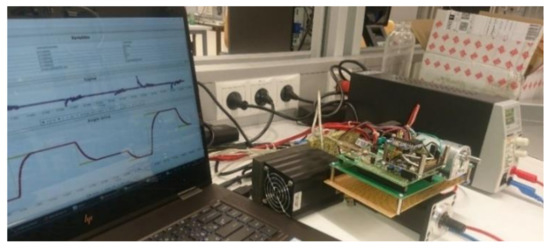
Figure 1.
Position system.
Nominal parameters were selected regarding the nominal operation point of the electro-mechanical system with mechanical constraints. Variables were measured in and , respectively. The desired value derivatives were assumed to be limited . Three different controllers were validated in the real-time experiment. The first controller had the same structure as (9) and was executed with a fixed sampling time .
The controllers and were executed in ET mode. The controller’s output was transformed to a PWM signal with the frequency of and duty-cycle range of , which corresponded to the supply voltage of ±24 V and voltage resolution of . Maximal velocity was . The controller parameters are presented in Table 1.

Table 1.
Controller parameters, , , .
The inter-event time and (26), (34) were estimated assuming that the closed-loop system was stabilized and the error . If an error was small regarding the selected controller parameters in Table 1, the approximate lower bound of the inter-event time was estimated to be 21 ms.
The closed-loop performance was evaluated with indices,
where is the number of triggering events for controllers and . The comparisons among the different techniques are presented in Figure 2, Figure 3, Figure 4 and Figure 5. Figure 2 presents the tracking capability of the step signal for controllers , and , RPM values, and controllers’ output.
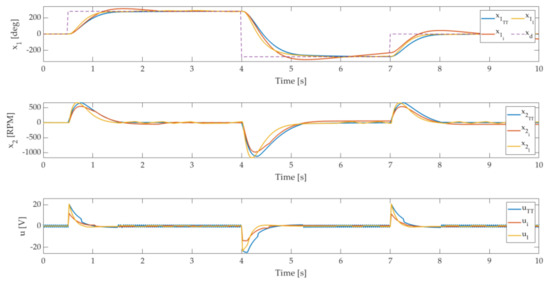
Figure 2.
Tracking capability comparison of TT and ET techniques, with variables , controllers’ output , and .
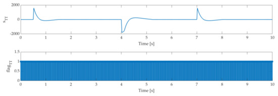
Figure 3.
Sliding variable evolution of the closed-loop system with controller and fixed sa-mpling time .
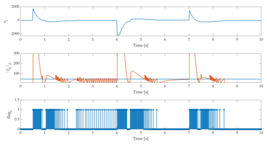
Figure 4.
ET sliding variable evolution with triggering condition and update flagi of the closed-loop system with the controller .
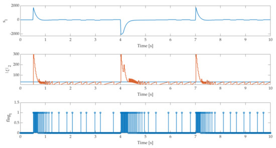
Figure 5.
ET sliding variable evolution with triggering condition and update flags of the closed-loop system with the controller .
Figure 3 presents the sliding variable evolution with update flags in the TT execution mode with a fixed sampling time of . Flag value 1 means that the controller is updated. Otherwise, the last value is preserved, and the flag equals zero.
Figure 4 presents the sliding variable evolution , triggering condition (16) with an error value , and update flags in ET execution mode with the controller .
Figure 5 presents the sliding variable evolution with triggering condition (23) and error value with the controller .
The indices values (36), (37) are presented in Table 2.
Table 2.
Performance indices of different controllers in TT and ET manner.
Figure 2, Figure 3, Figure 4 and Figure 5 compare the different implementation techniques of SMC controllers. It can be seen that the ET approach can be an efficient alternative to classic TT implementation of the controller algorithms. The system tracking capabilities have similar transient responses, especially by the approach with and controller , where the difference is not noticeable. The controller performance has limited tracking capability, which can be noticed in Figure 1 with a small steady-state error. The main reason for lower accuracy is a triggering rule structure (16) based only on a partial state vector for the presented system only on the state . The accuracy can be improved by lowering the parameters , which shortens the inter-event time and increases the demand of the algorithm update.
Both ET implementations reduce the burden of the real-time system significantly, which is evident in Figure 4 and Figure 5 and regarding Figure 3 with TT execution. In both ET approaches, the SMC property is preserved, showing the courses of the sliding variables and comparing . The percent of the update flags for the ET approach was calculated as the ratio of the number of executed flags (flagi, flagl) and experiment time duration regarding the ratio of TT execution flags per experiment time, which was evaluated as 100%. It is clear that both ET approaches overperformed the TT in the manner of the computation burden of the real-time system. The measured lower inter-event times and were much longer than the sampling time , which, regarding the closed-loop performance of the controller , increased the efficiency of the system resource usage drastically and preserved the closed-loop performance.
Table 2 presents the RMS values of the approach. It was expected that the RMS value of TT implementation would have a lower value regarding the ET approaches, which is a consequence of the triggering boundary and extended update time. The real-time data shows that the ET approach’s output variables did not exceed the boundary of 1degree for a system with and 0.4 deg for the system with , where the TT boundary was smaller than 0.1 deg. The real-time experiment confirmed that the ET technique is a trade-off between system accuracy and the computational burden. The efficiency of the ET-SMC with controller regarding is evident in the transient response, tracking capability, and the number of update flags. The proper selection of the coefficient lowers the output boundary and improves the dynamic of the closed-loop system.
Figure 6, Figure 7 and Figure 8 present the tracking capability to the periodic references signal. Figure 6 presents the tracking capability of the sine function for controllers , , , RPM values, and controllers’ output.
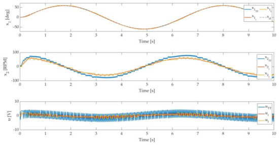
Figure 6.
Tracking capability comparison of TT and ET techniques to the periodic signal .
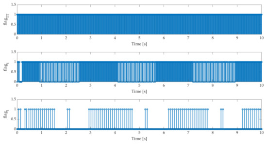
Figure 7.
Update flags of the controllers , and .
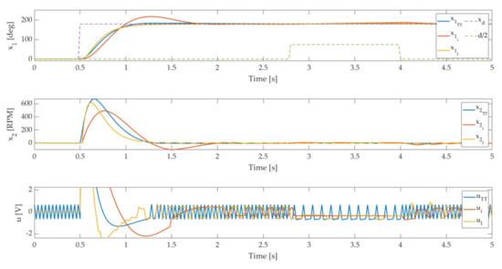
Figure 8.
Disturbance rejection of , and .
Figure 7 presents the update flags of the controllers , and .
The accuracy of the tracking capability to the periodic signal was ensured for all three approaches. In Figure 6 it can be noticed that the controller output produces less alternating voltage, which is beneficial for the positioning system. The chattering phenomena evident in Figure 2 and Figure 7 by the controller are significantly reduced with controllers and . The advantage of the controller is confirmed with results in Figure 7. The sequences of the update flags are longer than by controllers and . Figure 8 presents the responses to the matched disturbance signal. The disturbance is generated inside the embedded system, added to the controller’s output, and set to the value . The value is selected regarding the controller gain .
Figure 9 presents controllers’ updated flags during disturbance presence.
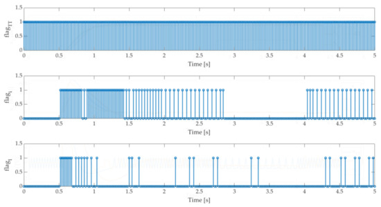
Figure 9.
Update flags of controllers , and during disturbance rejection test.
The disturbance capability of the SMC is ensured with the selection of the nonlinear function gain. The results confirm that the ET-SMC still preserves the SCM property if the disturbance is bound with the known value. The update flags show the advantage of and proposed structure. For the controller , the disturbance value forces the state error into a triggering bound, therefore no update occurs.
6. Conclusions
The paper presents an SMC event-triggered controller design for the class of dynamic systems with output integral behavior. For dynamic systems which do not possess the property of the fully connected canonical form, the induced triggering rule is based on a partial state vector, which does not include the output variable. Additional linear or nonlinear feedback terms in the controller`s structure, which involves the output variable, benefit the triggering rule with the fully informed system and closed-loop performance improvements. As we have presented with the experimental results, the improvements are evident in the closed-loop dynamics, tracking capability, and inter-event time extension. The paper shows the property of the ET approach with a comparison to the classic TT implementation. The trade-off is presented between computational burden and system accuracy. The possibility of embedded system task scheduling is possible. The triggering rule can be validated regarding the estimated inter-event time, where the presented computational complexity of the rule validation is low and does not require a long processing time.
The additional improvements of the presented ET approach can be achieved regarding the integral behavior of the system. When the system approaches the equilibrium point, it is known that the controller output convergence is zero. In this case, an additional proactive adaptation rule can be applied. The triggering rule can be extended with the absolute triggering technique, where the final value of the desired signal regarding the prescribed vicinity of the output variable triggers the update and sets the controller to zero. The system will remain in the attraction region of the sliding manifold until the desired value is changed or disturbance has occurred, and no additional updates of the controller are needed.
Author Contributions
Conceptualization, A.S. and D.G.; methodology, D.G. and A.S.; software, A.S.; validation, A.S.; formal analysis, A.S. and D.G.; investigation, D.G. and A.S.; writing—original draft preparation, A.S.; writing—review and editing, D.G.; visualization, A.S.; supervision, D.G.; funding acquisition, D.G. All authors have read and agreed to the published version of the manuscript.
Funding
This research was funded by the Slovenian Research Agency (ARRS) Grant number P2-0065.
Institutional Review Board Statement
Not applicable.
Informed Consent Statement
Not applicable.
Data Availability Statement
Not applicable.
Conflicts of Interest
The authors declare no conflict of interest.
References
- Franklin, G.F.; Powell, J.D.; Workman, M.L. Digital Control of Dynamic Systems, 3rd ed.; Addison Wesley: Menlo Park, CA, USA, 1997. [Google Scholar]
- Proakis, J.G.; Manolakis, D.G. Digital Signal Processing: Principles, Algorithms, and Applcations; Prentice Hall: Upper Saddle River, NJ, USA, 2007. [Google Scholar]
- Phillips, C.L.; Nagle, H.T.; Chakrabortty, A. Digital Control System Analysis and Design, 4th ed.; Pearson: Essex, UK, 2015. [Google Scholar]
- Kuo, B.C. Digital Control Systems, 2nd ed.; Oxford University Press: Oxford, UK, 1995. [Google Scholar]
- Bemporad, A.; Heemels, H.; Johansson, M. Networked Control Systems; Springer: Berlin/Heidelberg, Germany, 2010. [Google Scholar]
- Murthy, C.S.R.; Manimaran, G. Resource Management in Real-time Systems and Networks; The MIT Press: Cambridge, MA, USA, 2001. [Google Scholar]
- Bernhardsson, B.; Åström, K.J. Comparison of periodic and event-based sampling for first-order stochastic systems. In Proceedings of the 14th IFAC World Congress, Beijing, China, 5–9 July 1999. [Google Scholar]
- Årzén, K.-E. A simple event-based pid controller. In Proceedings of the 14th IFAC World Congress, Beijing, China, 5–9 July 1999. [Google Scholar]
- Antunes, D.; Heemels, W.P.M.H. Rollout event-triggered control: Beyond periodic control performance. IEEE Trans. Autom. Control 2014, 59, 3296–3311. [Google Scholar] [CrossRef]
- Girard, A. Dynamic triggering mechanisms for event-triggered control. IEEE Trans. Autom. Control 2015, 60, 1992–1997. [Google Scholar] [CrossRef] [Green Version]
- Wu, W.; Reimann, S.; Gorges, D.; Liu, S. Suboptimal event-triggered control for time-delayed linear systems. IEEE Trans. Autom. Control 2015, 60, 1386–1391. [Google Scholar] [CrossRef]
- Behera, A.K.; Bandyopadhyay, B.; Cucuzzella, M.; Ferrara, A.; Yu, X. A Survey on Event-Triggered Sliding Mode Control. IEEE J. Emerg. Sel. Top. Ind. Electron. 2021, 2, 206–217. [Google Scholar] [CrossRef]
- Behera, A.K.; Bandyopadhyay, B. Event-triggered sliding mode control for a class of nonlinear systems. Int. J. Control 2016, 89, 1916–1931. [Google Scholar] [CrossRef]
- Behera, A.K.; Bandyopadhyay, B.; Yu, X. Periodic event-triggered sliding mode. Automatica 2018, 96, 1916–1931. [Google Scholar] [CrossRef]
- Incremona, P.G.; Ferrara, A. Adaptive model-based event-triggered sliding mode control. Int. J. Adapt. Control Signal Process. 2016, 30, 1298–1316. [Google Scholar] [CrossRef]
- Hou, H.; Yu, X.; Fu, Z. Sliding Mode Control of Networked Control Systems: An Auxiliary Matrices Based Approach. IEEE Trans. Autom. Control 2021, 51. [Google Scholar] [CrossRef]
- Hou, H.; Yu, X.; Xu, L.; Rsetam, K.; Cao, Z. Finite-Time Continuous Terminal Sliding Mode Control of Servo Motor Systems. IEEE Trans. Ind. Electron. 2020, 67, 5647–5656. [Google Scholar] [CrossRef]
- Shtessel, Y.; Edwards, C.; Fridman, L.; Levant, A. Sliding Mode Control and Observation; Springer: Berlin/Heidelberg, Germany, 2014. [Google Scholar]
- Tabuada, P. Event-triggered real-time scheduling of stabilizing control tasks. IEEE Trans. Autom. Control 2007, 52, 1680–1685. [Google Scholar] [CrossRef] [Green Version]
- Moreno, J.A.; Osorio, M. Strict Lyapunov functions for the super-twisting algorithm. IEEE Trans. Autom. Control 2008, 57, 1035–1040. [Google Scholar] [CrossRef]
- Igrec, D.; Chowdhury, A.; Štunberger, B.; Sarjaš, A. Robust tracking system design for a synchronous reluctance motor—SynRM based on a new modified bat optimization algorithm. Appl. Soft Comput. 2018, 69, 568–584. [Google Scholar] [CrossRef]
- Bartolini, G.; Ferrara, A.; Pisano, A.; Usai, E. Adaptive reduction of the control effort in chattering-free sliding-mode control of uncertain nonlinear systems. Appl. Math. Comput. Sci. 1998, 8, 51–71. [Google Scholar]
- Boiko, I.; Fridman, L. Analysis of chattering in continuous sliding mode controllers. IEEE Trans. Autom. Control 2005, 50, 1442–1446. [Google Scholar] [CrossRef] [Green Version]
- Soriano, L.A.; Rubio, J.D.J.; Orozco, E.; Cordova, D.A.; Ochoa, G.; Balcazar, R.; Cruz, D.R.; Meda-Campaña, J.A.; Zacarias, A.; Gutierrez, G.J. Optimization of Sliding Mode Control to Save Energy in a SCARA Robot. Mathematics 2021, 9, 3160. [Google Scholar] [CrossRef]
- Wang, G.; Wang, B.; Zhang, C. Fixed-Time Third-Order Super-Twisting-like Sliding Mode Motion Control for Piezoelectric Nanopositioning Stage. Mathematics 2021, 9, 1770. [Google Scholar] [CrossRef]
- Obeid, H.; Fridman, L.; Laghrouche, S.; Harmouche, M. Barrier Function-Based Adaptive Sliding Mode Control. Automatica 2018, 93, 540–544. [Google Scholar] [CrossRef]
- Utkin, V.; Guldner, J.S. Sliding Mode Control in Electromechanical Systems; Taylor & Francis Ltd: London, UK, 1999. [Google Scholar]
- Rivera, J.D.; Mora-Soto, C.; Ortega, S.; Raygoza, J.J.; De La Mora, A. Super-twisting control of induction motors with core loss. In Proceedings of the 11th International Workshop on Variable Structure Systems (VSS), Mexico City, Mexico, 26–28 June 2010; pp. 428–433. [Google Scholar]
- Utkin, V. Discussion aspects of high-order sliding mode control. IEEE Trans. Autom. Control 2016, 61, 829–833. [Google Scholar] [CrossRef]
- Ventura, U.P.; Fridman, L. Design of super-twisting control gains: A describing function based methodology. Automatic 2019, 99, 175–180. [Google Scholar] [CrossRef]
- Yu, X.; Feng, Y.; Man, Z. Terminal Sliding Mode Control—An Overview. IEEE Open J. Ind. Electron. Soc. 2021, 2, 36–52. [Google Scholar] [CrossRef]
- Castillo, I.; Freidovich, L. Barrier Sliding Mode Control and On-line Trajectory Generation for the Automation of a Mobile Hydraulic Crane. In Proceedings of the 15th International Workshop on Variable Structure Systems (VSS), Graz, Austria, 9–11 July 2018; pp. 162–167. [Google Scholar] [CrossRef]
- Moreno, J.A.; Osorio, M. A Lyapunov approach to second-order sliding mode controller and observer. In Proceedings of the 47th IEEE Conference on Decision and Control, Cancun, Mexico, 9-11 December 2008; pp. 2856–2861. [Google Scholar]
- Gao, W.; Wang, Y.; Homaifa, A. Discrete-time Variable Structure Control System. IEEE Trans. Ind. Electron. 1995, 42, 117–122. [Google Scholar]
- Bartoszewicz, A. Discrete-time quasi-sliding-mode control strategie. IEEE Trans. Ind. Electron. 1998, 45, 633–637. [Google Scholar] [CrossRef]
- Koch, S.; Reichhartinger, M. Discrete-time equivalents of the super-twisting algorithm. Automatica 2019, 107, 190–199. [Google Scholar] [CrossRef]
- Brogliato, B.; Polyakov, A. Digital implementation of sliding-mode control via the implicit method: A tutorial. Int. J. Robust Nonlinear Control 2021, 31, 3528–3586. [Google Scholar] [CrossRef]
- Mojallizadeh, M.R.; Brogliato, B. Time-discretizations of differentiators: Design of implicit algorithms and comparative analysis. Int. J. Robust Nonlinear Control 2021, 31, 7679–7723. [Google Scholar] [CrossRef]
- Behera, A.K.; Bandyopadhyay, B. Self-triggering based sliding-mode control for linear systems. IET Control Theory Appl. 2015, 9, 2541–2547. [Google Scholar] [CrossRef]
- Behera, A.K.; Bandyopadhyay, B. Steady-state behaviour of discretized terminal sliding mode. Automatica 2015, 54, 176–181. [Google Scholar] [CrossRef]
- Cucuzzella, M.; Ferrara, A. Practical second-order sliding modes in single-loop networked control of nonlinear systems. Automatica 2018, 89, 235–240. [Google Scholar] [CrossRef] [Green Version]
- Filippov, A.F. Differential Equations with Discontinuous Righthand Sides; Springer Science Business Media: Berlin, Germany, 2013. [Google Scholar]
Publisher’s Note: MDPI stays neutral with regard to jurisdictional claims in published maps and institutional affiliations. |
© 2022 by the authors. Licensee MDPI, Basel, Switzerland. This article is an open access article distributed under the terms and conditions of the Creative Commons Attribution (CC BY) license (https://creativecommons.org/licenses/by/4.0/).