Abstract
Even while the scientific community has shown great interest in the analysis of meta-heuristics, the analysis of their parameterization has received little attention. It is the parameterization that will adapt a meta-heuristic to a problem, but it is still performed, mostly, empirically. There are multiple parameterization techniques; however, they are time-consuming, requiring considerable computational effort and they do not take advantage of the meta-heuristics that they parameterize. In order to approach the parameterization of meta-heuristics, in this paper, a self-parameterization framework is proposed. It will automatize the parameterization as an optimization problem, precluding the user from spending too much time on parameterization. The model will automate the parameterization through two meta-heuristics: A meta-heuristic of the solution space and one of the parameter space. To analyze the performance of the framework, a self-parameterization prototype was implemented. The prototype was compared and analyzed in a SP (scheduling problem) and in the TSP (traveling salesman problem). In the SP, the prototype found better solutions than those of the manually parameterized meta-heuristics, although the differences were not statistically significant. In the TSP, the self-parameterization prototype was more effective than the manually parameterized meta-heuristics, this time with statistically significant differences.
1. Introduction
In optimization there are problems that cannot be solved efficiently, that is, it is necessary to enumerate, implicitly or explicitly, the solutions, to find the optimum. The enumeration of solutions is inefficient, laborious and impractical. This is particularly important because most complex optimization problems are COPs (combinatorial optimization problems), susceptible to combinatorial explosion. In other words, susceptible to a rapid increase in the number of solutions with an increase in the size of the problem. One answer to complex COPs is the use of approximate techniques, that is, techniques that do not always find the optimal solutions, but unlike the enumeration techniques, are efficient. Among the approximate techniques, it is important to highlight meta-heuristics. Meta-heuristics are equipped with mechanisms that allow them to overcome the limitations of other approximate techniques.
Even if meta-heuristics can be considered the ideal approximate techniques for complex optimization problems, there are obstacles to their implementation. One obstacle is the impact of parameterization on their performance. One meta-heuristic performance cannot be disassociated from the parameterization procedure, that is, it is impossible to assess the appropriateness of the meta-heuristic to a problem without considering the parameterization. It is the parameterization that allows a meta-heuristic to be adapted to a problem, or even to an instance of the problem. In other words, it is the parameters that tune the meta-heuristic to the desired performance, weighing the intensification/diversification of the exploration of the space of solutions.
Although the parameterization influences the performance of the meta-heuristic, it is still common for the parametrization to be performed empirically, based on the knowledge the user has of a given meta-heuristic. Even though there are multiple parameterization methods, most require considerable effort in parameterization or involve the application of complex parameterization techniques. When faced with a complex problem, one does not only need to implement a meta-heuristic, but spend a lot of time on parameterization, or use a method that can be more complex than the meta-heuristic itself.
In this paper, the authors intend to contribute to the automation of the parameterization of meta-heuristics, reducing the user’s intervention to a minimum. In order not to increase the complexity of the parameterization process, a meta-heuristic will be used in the parameterization procedure. Our self-parametrization framework uses two meta-heuristics, a meta-heuristic of the parameter space and a meta-heuristic of the solutions space. In order to evaluate the framework, a self-parametrization prototype was compared with a well-established parameterization method in the computational study.
This paper is organized as follows: Section 1 is the introduction, Section 2 and Section 3 are literature review. Section 2 is a brief introduction to meta-heuristics and Section 3 an in-depth review of parametrization techniques. Section 4 presents the proposed self-parametrization framework. Section 5 presents the results of computational study and Section 6 examines the results. Section 7 presents the conclusions.
2. Meta-Heuristics
Meta-heuristics are approximate techniques that can be applied to almost all optimization problems, regardless of their size or complexity. In fact, meta-heuristics have been accepted as the only realistic approach for optimization problems that are too complex. For example, in scheduling operations, Xhafa & Abraham [1] claim that “meta-heuristics have become a de facto approach to tackle in practice with the complexity of scheduling problems.”
In [2], meta-heuristics are defined as techniques that control subordinate heuristics in the search of solution space. In other words, approximate techniques, developed to overcome the limitations of other approximate techniques. Even the name “meta-heuristic” is not consensual. In [3], Sean Luke states that the name meta-heuristics is “An unfortunate term, often used to describe a subfield of stochastic optimization.” It is worth mentioning that several authors, including [4], classify local search as a meta-heuristic and neither steepest-descent or first-descent are stochastic. In this paper, meta-heuristics are defined as approximate techniques, equipped with stochastic mechanisms to overcome local optimums. In that context, local search is not considered a meta-heuristic.
In [5], the properties of meta-heuristics are presented: first, meta-heuristics can be applied to almost all problems; second, they incorporate mechanisms to overcome local optimums; third, they use experience to direct the search of the solutions space. In short, they must be applicable to almost all problems with few, if any, modifications, they must be efficient and they must use the information collected to direct their search of the solutions space. In other words, meta-heuristics are flexible techniques that make a compromise between the effectiveness of the solution and the efficiency of search. For problems where it is time consuming to enumerate the solutions, and the other approximate techniques are ineffective, meta-heuristics compromise between effectiveness and efficiency.
It is important to mention the contrast between intensification and diversification, which is essential to understand how a meta-heuristic will approach a problem. Intensification is the comprehensive exploration of the most auspicious areas of the solution space while diversification maintains the overall perspective of the solution space. It is the intensification/diversification balance that allows meta-heuristics to move past local optimums. If a meta-heuristic has too much intensification it will stop on the nearest local optimum. On the other hand, if a meta-heuristic has too much diversification it becomes inefficient and almost identical to a random search [5]. It is the parameterization that balances the intensification/diversification, that is, it is the parameterization that will determine how much intensification/diversification the meta-heuristic has.
Some of the better-known meta-heuristics are: Genetic Algorithms (GA), proposed by Holland [6] in 1975; Simulated Annealing (SA), independently developed by Kirkpatrick et al. [7] and Černý [8] in the 1980s; Tabu Search (TS), proposed by Glover in 1986 [9]; GRASP, proposed by Feo & Resende [10]; the Variable Neighborhood Search (VNS), proposed by Mladenocić & Hansen [11]; the Iterated Local Search (ILS) proposed by Stützle [12]; Dorigo’s Ant Colony Optimization (ACO) [13], Kennedy & Eberhard’s Particle Swarm Optimization (PSO) [14] and the Bacterial Foraging Optimization Algorithm (BFOA), proposed by Passino [15]. Other meta-heuristics include: The Firefly Algorithm (FA), Cuckoo Search (CS) and the Bat Algorithm (BT), developed by Yang [16,17,18]; Grey Wolf Optimizer (GWO) proposed by Mirjalili et al. [19] and later adapted for discrete problems in [20]. Other meta-heuristics have been adapted to better suit specific problems; one example is the recent variation of CS presented in [21].
One recent trend is the development of “hybrid” meta-heuristics. One oldest “hybrid” meta-heuristic is the Memetic Algorithm (MA), proposed in 1989 [22]. It combines an evolutionary meta-heuristic with local search. In addition, the combination of meta-heuristics with mathematical models, math-heuristics, have also been studied [23]. Another trend is the combination of meta-heuristics with other AI (Artificial Intelligence) techniques, particularly, ML (Machine Learning). One unfortunate trend is the focus on the inspiration in natural phenomenon [24], with multiple meta-heuristics with similar procedures. In the meantime, the parametrization continues to be understudied.
While much could be said about the recent developments in meta-heuristics and their applications, since the bulk of the literature review is presented in Section 3 any further expansion of Second 2 would make the paper unnecessarily dense.
Discrete Artificial Bee Colony
Bees have inspired multiple meta-heuristics, including Queen-Bee Evolution (QBE) [25], Marriage in Honey Bees Optimization (MBO) [26], Bee Colony Optimization (BCO) [27], Virtual Bee Algorithm (VBA) [28] and others [29]. One of the best-known is Artificial Bee Colony (ABC), developed by Karaboga [30] and Pham et al. [31]. ABC uses three categories of bees to search for solutions, worker bees, onlooker bees and scout bees. Although ABC was developed for continuous problems, there are adaptations of ABC for discrete problems, including the Discrete Artificial Bee Colony (DABC), proposed in [32].
DABC procedure is similar to the ABC, but bees explore discrete solutions. Food sources represent solutions. Worker bees explore food sources, onlooker bees wait in the hive and choose and explore the most promising food sources, and finally, scout bees look for new food sources. As the most promising food sources will attract more onlooker bees, they will be explored more meticulously than other food sources.
In detail, DABC, and ABC, repeat three phases until the search is interrupted. First, each worker bee is allocated to a food source (s0), then the phases of worker, onlooker and scout bees are repeated. In the worker bee phase, bees explore a solution (si′), in the vicinity of the food source (si) to which they have been allocated. If the candidate solution (si′) is better than the food source, then the new solution replaces the food source (si). In the onlooker bee phase, bees will wait for the performance of each food source (si), before selecting one. After selecting a food source, the bees will explore a solution (si′) in the vicinity of the selected food source (si). If the candidate solution (si′) is better than the food source, then it replaces that food source (si). Finally, the scout bee phase occurs when a food source is abandoned. If a food source is abandoned, then, the worker bee is transformed into a scout bee and searches for a new food source [16].
DABC parameters are the hive size (L) and the limit number (l). Hive size determines how many bees there are, in other words, how many solutions are explored per iteration. An excessive L will make DABC inefficient. On the other hand, the limit number determines when a food source is abandoned, that is, the number of iterations without improvement until a food source is abandoned [16]. DABC is presented in Table 1.

Table 1.
Discrete Artificial Bee Colony.
Other versions of DABC have been developed. In [33,34,35] three versions of the DABC can be examined, with variations in the procedure. In [36], an adapted version of the DABC was used to address the TSP, and in [37], it was used to solve a manufacturing cell design problem (MCDP). The performance of DABC and Simulated Annealing (SA), were compared in a single machine scheduling problem [38]. DABC obtained better solutions than SA, but it needed more computational time.
One of the variations of DABC is related to how onlooker bees choose food sources. In [32], it is proposed that part of the probability is not impacted the by quality of the solution. In other words, the onlooker bees will not only consider the amount of food in a food source, which should increase the diversification.
3. Parametrization of Meta-Heuristics
For meta-heuristics, parameterization can be described as: for an optimization technique A, an instance of problem I, with a performance index C, which parameters of A optimize C in I [39]. In other words, what are the parameters that will result in the best performance of the meta-heuristic in an instance of a problem. It is inexplicable how parametrization has been so understudied, when the performance of meta-heuristics depends so much on it. Manual parametrization is still predominant, with parameters selected empirically, when they are even reported [40]. It is common to report on the performance of a meta-heuristics with “certain” parameters. Why or how were these parameters selected? It is rarely explained [41]. To ensure the best performance from a meta-heuristic, it is necessary to select the correct parameters for the problem, or even, the instance.
Parameterization can be offline or online. Offline is when the parameters of the meta-heuristic are predetermined and online is when the parameters are updated as the meta-heuristic is executed [4]. In other words, offline parametrization, which is the focus of this paper, is performed a priori. It can be divided into: manual parametrization, parametrization by analogy, parametrization by DOE and search-based parametrization [42].
3.1. Manual Parametrization
In manual parameterization the parameters are iteratively tweaked. Manual parameterization does not require a careful plan of experiments but needs a user who is familiar with the meta-heuristic. It is a simple procedure: the user runs the meta-heuristics with some initial parameters, which are tweaked one by one to improve the performance until the user is satisfied with the performance of the meta-heuristic [42]. It is a laborious procedure that depends on the user’s acquaintance with the meta-heuristic. One representation of manual parametrization is presented in Figure 1. Once the initial parameters have been determined (1), the user evaluates the performance (2), the parameters are tweaked (3) and the procedure is repeated (4). Manual parametrization is inconsistent, since it does not consider the interactions between parameters, but it is still the most common parameterization technique [43].
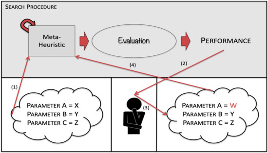
Figure 1.
Manual Parametrization.
3.2. Parametrization by Analogy
In parametrization by analogy users search for successful implementation of the meta-heuristic and replicate the parameters. One representation of parametrization by analogy is presented in Figure 2. Before the user runs the meta-heuristic (1), they will search for successful implementations of the meta-heuristic (2), find what parameters were used (3) and apply those parameters (4).
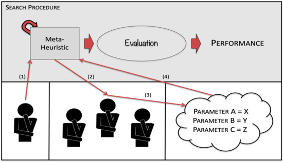
Figure 2.
Parametrization by Analogy.
3.3. Parametrization by DOE
In parametrization by DOE users choose the parameters in multiple experimental trials. One representation of parametrization by DOE is presented in Figure 3. Before the user runs the meta-heuristic, multiple parameterization trials are executed (1), then, the user chooses the parameters with the best performance (2) and applies them to the meta-heuristic (4).
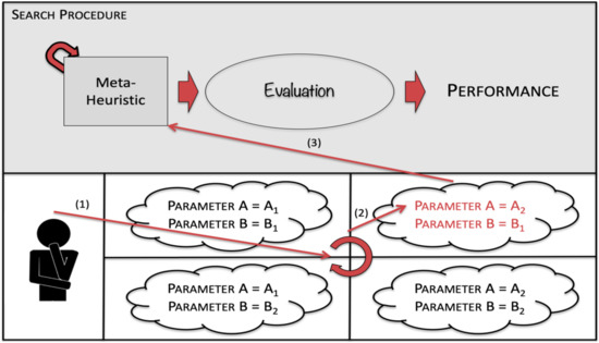
Figure 3.
Parametrization by DOE.
Parametrization DOE is the methodical and statistical examination of experiments [44]. Input variables are tweaked, and the output is evaluated [45]. OFAT (one factor at a time) is when one input variable is tweaked per experiment. It does not consider the interactions between the variables. DOE is the alternative, which examines the interaction between the variables in the output. In [46] DOE is divided into classical experiments, Taguchi experiments or Shainin experiments.
Classical experiments uses the concepts developed by Fisher [47] to evaluate the output sensitivity to the input parameters. Complete factorial experiments, which are only useful when there are few parameters, consider all the interaction between the inputs [46]. In order to reduce the number of experiments, fractional factorial experiments were developed. While complete factorial experiments will examine each combination of parameters, fractional factorial experiments will only perform a fraction of the experiment with orthogonal arrays. Response surface methodology (RSM), developed by Box and Wilson [48], is, for example, a form of classical experiment. On the other hand, Taguchi experiments, which use orthogonal arrays, focus on the reduction in the variance of the outputs [49]. In order to reduce variance in the response to the inputs, they are classified into control and noise inputs [50]. Control inputs are, for example, the parameters of a meta-heuristic, while the noise inputs cannot be controlled, for example, the differences between instances. Taguchi experiments search for the control inputs that allow the meta-heuristic to withstand the uncontrollable variation of the noise inputs. Other parametrization by DOE techniques such as F-Race and Sequential Parameter Optimization (SPO), can be found in [51,52,53,54,55,56,57,58,59,60,61,62,63,64].
3.4. Search based Parametrization
In search-based parametrization, the parameterization is approached as a meta-optimization problem [4]. In other words, the space of the parameters is explored by an approximate technique, such as local search or a meta-heuristic [42]. One representation of search-based parametrization is presented in Figure 4. Before the user runs the meta-heuristics (1), they first use an approximate technique to explore the space of the parameters (2) and then use those parameters in the meta-heuristics (3).
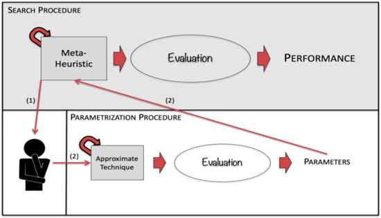
Figure 4.
Search-based Parametrization.
One successful implementation of search-based parametrization was presented in 1986, when a Meta-GA was applied in the parameterization of the Genetic Algorithm (GA). In that case, the Meta-GA was used to explore GA’s parameter space, which, in turn, would explore the solution space [65]. Since the same meta-heuristics was used in the parameterization and optimization, the user did not need to implement a technique developed specifically to solve the parameterization problem. It was a smart solution, which inspired the proposed self-parametrization framework.
One similar approach is relevance estimation and value calibration (REVAC), proposed by Nannen & Eiben [66]. REVAC uses an evolutionary algorithm (EA) to estimate the parameters of another EA. It starts from a population of calibrations and will explore the space of the parameters. Like all EAs, it will use the best solutions, in this case the best calibrations, to find even better calibrations. The REVAC procedure is simple: It starts with a population of parameter vectors, that is, calibrations for the EA used in the optimization problem. REVAC will then improve those vectors iteratively. At the start, the probability distribution is uniform, however, REVAC will increase the probability of the vectors that result in better performance of the EA [67]. At the same time, REVAC will smooth the probability distribution of the vectors, to reduce the variance in the performance of the parameters.
Parameter iterated local search (ParamILS) is a search-based parametrization proposed by Hutter et al. [39]. It is similar to manual parametrization, since it will manipulate the parameters one-by-one, that is, ParamILS does not consider iterations between parameters but uses local search to explore the parameter space [42]. The ParamILS procedure is simple: it will tweak one parameter and see if it results in a better solution for the optimization problem. In order to overcome the local optimums, disturbance mechanisms were introduced. ParamILS will repeat these two phases, local search and disturbances. First it does a local search and once it reaches a local optimum it causes a disturbance to restart the search. It more flexible than REVAC, since ParamILS is not limited to quantitative parameters. In [39], two variations of ParamILS were proposed: BasicILS and FocusedILS.
3.5. Other Parametrization Techniques
As an alternative approach, it is common to “mix” parameterization techniques. For example, when the interruption criteria are determined by manual parametrization and the other parameters are determined by parametrization by analogy. Another common combination is parameterization by analogy with parameterization by DOE, since it is necessary to determine levels for the parameters for the experiments. Even search-based parameterization could need to levels for parameters, which can be selected by manual parametrization or parametrization by analogy.
It is also important to mention Calibra, which is a parameterization technique that combines parameterization by DOE and search-based parametrization [68]. It will refocus the parametrization experiments in the best zones of the parameter space. It determines a parameter interval and performs a complete factorial experiment of the values of the first and third quartile of the parameter interval or it will perform 2k experiments, where k represents the number of parameters. Once those experiments are completed, it will define three levels for each parameter and use local search to decrease the interval of each parameter. One of the limitations of Calibra is the fact that it only calibrates up to four parameters, since it was developed with a L9 orthogonal arrays.
4. Self-Parametrization Framework
In this section, the self-parametrization framework will be presented, but first, what would be the purpose of self-parametrization framework? It should find the appropriate parameters for all meta-heuristics, in all instances of all problems, without user intervention. It would, also, remove the parameterization burden from the user of the meta-heuristic which, in turn, would allow inexperienced users to solve problems that could not be solved otherwise. Even the more experienced users could benefit from a self-parametrization framework and avoid the laborious parametrization procedure. One could run the self-parametrization module and tune the parameters of the meta-heuristic to the problem, or even to the instance, and avoid the all the experiments and the search in literature for recommendations for the values of the parameters. Moreover, if the self-parameterization is implemented it can help in the development of decision support systems (DSS), where the parameters are not pre-defined for a problem, or a specific instance of the problem.
With the self-parametrization framework parameters are tweaked as if the parameterization was an optimization problem. In order to automate the parameterization procedure, the self-parametrization framework will use two meta-heuristics. One is the meta-heuristic of the solution space and the other is the meta-heuristic of the parameter space. It is the second that will search for complete calibrations, which in turn are evaluated with runs of the meta-heuristic of the solution space. In essence, the meta-heuristic of the parameter space searches for solutions for the parametrization problem and the meta-heuristic of the solutions space evaluates the solutions. Solutions from the meta-heuristic of the parameter space are complete calibrations of the meta-heuristic of the solution space, whose performance is used to calculate the quality of those calibrations. Once the meta-heuristic of the solution space receives a calibration, it runs in the optimization problem before returning the solutions to the meta-heuristic of the parameters space, which will tweak the parameters and repeat the whole procedure.
In Figure 5 the procedure of the self-parametrization framework is presented.
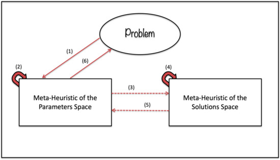
Figure 5.
Self-Parametrization Framework.
First, the problem’s data is sent to the meta-heuristic of the parameter space (1), then, the meta-heuristic of the parameter space will examine the problem’s data and limit the parameter space, before it starts to search for a calibration solution (2). Once it has found a calibration solution, that calibration is sent to the meta-heuristic of the solution space (3), which will search in the solution space with that calibration (4), before it returns the solution of the problem to the meta-heuristic of the parameter space (5). Steps (2), (3), (4) and (5) are repeated until the interruption criterion of the meta-heuristic of the parameter space, and in 6, the meta-heuristic of the parameter space will recommend a calibration for the problem to the user of the self-parametrization framework. In addition, the self-parameterization framework will report the solution for the optimization problem.
One limitation of the self-parametrization framework is the representation of the parameters, since the parameters of a meta-heuristic can be continuous, discrete or a mixture of discrete and continuous. If a discrete meta-heuristic was used as the meta-heuristic of the parameters space, then, continuous parameters would need to be discretized. If a continuous meta-heuristic was used as the meta-heuristic of the parameters space it would be the opposite. Of course, the discretization of parameters represents a decrease in the resolution, but it’s a flexible solution that allows user to implement any meta-heuristic, as the meta-heuristic of the parameter space.
Another limitation of the self-parametrization framework is the evaluation of the calibrations. As mentioned, the meta-heuristic of the parameters space will use the meta-heuristic of the solution space to evaluate the performance of the calibrations, but since meta-heuristics are stochastic, bad calibrations can still result in decent solutions. In order to minimize this, the meta-heuristic of the parameters space needs to evaluate calibrations in multiple runs of the meta-heuristic of the solutions space. The user would need to select if the calibration solution is evaluated by the best, worst or the mean solution for the optimization problem.
In Figure 6 the structure of the self-parametrization prototype is presented. DABC is as both the meta-heuristic of the parameters space and the meta-heuristic of the solutions space.
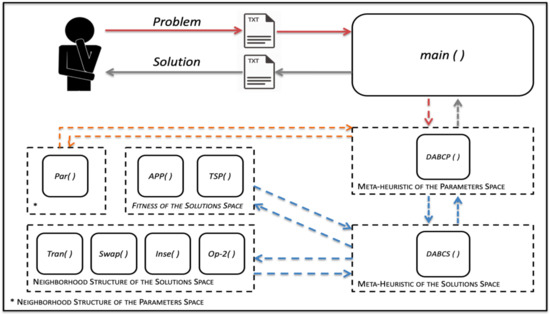
Figure 6.
Self-Parametrization Prototype.
It can be divided into parameterization modules, which are: DABCP (); the neighborhood structure, Par (), which the meta-heuristic of the parameters space uses to manipulate the calibration solutions and the evaluation module, DABCS (). On the other hand, the optimization modules are: DABCS (); four neighborhood structure modules, Tran (), Swap (), Inse () and Op-2 (), which the meta-heuristic of the solution space uses to manipulate the solutions and the two evaluation modules, APP () and TSP (), since it will be tested in two problems. Main reports the calibration to the user, in a txt file.
5. Computational Study
In order to validate the proposed self-parametrization framework, it will be compared to conventionally parametrized frameworks, namely, parameterization by analogy and parametrization by DOE, DABC in two optimization problems. First, the self-parametrization framework will be tested in a scheduling problem (SP), in this case, the minimization of total weighted tardiness (TWT). TWT is often used to evaluate the performance of meta-heuristics. It will, also, be tested in TSP, in the case, a Euclidean/symmetrical-TSP, which is also a well-known problem, often used to evaluate meta-heuristics.
For both TWT and TSP, the instances are from well-known databases of optimization problems. In TWT, the proposed framework will be evaluated in 30 instances of 50 activities problem, available in the ORLibrary [69]. In the TSP, the proposed framework will be evaluated in the instances KroA100, KroB100, KroC100, KroD100 and KroE100, available in TSPLIB [70]. In both problems the proposed framework, will be compared to the performance of a conventionally parametrized DABC. Moreover, in other to ensure both the proposed framework and the conventionally parametrized DABC have found suitable solutions, SA was also included in the computational study. SA’s resilience to subpar parametrization is well-known [71,72,73]. Since SA is included as a baseline and it will not be included in the statistical comparison, its parametrization process will not be described.
In the future, it would be important to compare the proposed framework with other search-based and hybrid parameterization techniques. However, most search-based and hybrid parameterization methods were developed for specific meta-heuristics and were tested in the same instances as our framework. Such comparison would require implementation, and possible adaption of other complex techniques, which fall outside the scope of this paper. Moreover, other search-based and hybrid parameterizations are often inaccessible to users. Our framework does not require a separate parametrization algorithm and can be applied to any meta-heuristic, without much effort.
5.1. Parametrization
Before the parametrization of DABC it is necessary to mention the three parameters that have been proposed but are not used in all implementations of DABC. The first is the number of scout bees. In ABC [30] only one scout bee is allowed per iteration, but in [74] from 10% to 30% of scout bees are recommended per iteration. The second is the number of movements (NuMo) of a scout bee, before it turns back into a worker bee. In [34] at least three movements are recommended. Lastly, another parameter is proposed in this article, inspired by [32]. In [32], 10% of the probability of an onlooker bee selecting one food source is not impacted the quality of the food source. In this article we consider the part not impacted, hence the quality of the solution is 1-α, where α is the elitism percentage.
In the TWT problem the limit number (l), the neighborhood structure, the number of movements (NuMo) and the elitism percentage (α) will be parametrization first by parametrization by analogy and then, fine-tuned with parametrization by DOE, in this case, in three levels, with Taguchi experiments. On the other hand, hive size (L) and the interruption criteria, which will be the number of iterations, in order to ensure the fairness of the comparison between the proposed framework, the conventionally parametrized DABC and the conventionally parametrized SA, will be chosen in manual parametrization, before the other parameters are determined.
In [32], a hive size of 40 was used to solve a TS. In [33,34], a Hive Size of 20 was used to solve a SP. In [75], it is concluded that the ABC is not very sensitive to the hive size. For TWT problem will use a mean of the two values, in this case a hive size of 30. Since DABC will explore 30 solutions per iteration and in order to ensure the fairness of the comparison, DABC will be interrupted after 1000 iterations and SA after 30,000 iterations.
In [32] a metric is presented to calculate the limit number. For a hive size of 30, the levels of 450, 500 and 550 were chosen. For the elitist percentage, in [32], a value of 0.9 is proposed, therefore levels of 0.85, 0.90 and 0.95 were chosen. For the number of movements, in [34] at least three movements are recommended, so the levels of three four and five were chosen. Finally, the neighborhood structures chosen were Transpose, Swap and Insert. The Taguchi experiments, repeated for each of the first five instances of the problem, are presented in Table 2.
Table 2.
Taguchi Experiments for TWT Problem.
S/Ns are presented in Figure 7. It seems the neighborhood structure is the parameter with the most impact in the performance of DABC, due to the poor performance of Transponse, which is unappropriated for instances of this size. The limit number, elitist percentage and number of movements have more uniform results.
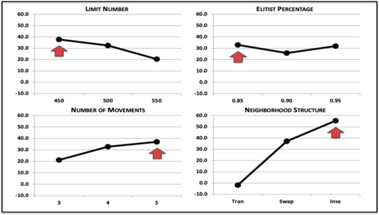
Figure 7.
Parametrization for TWT Problem.
For the TWT problem, SA will use an initial temperature (Tmax) of 45,000, an epoch length (L) of 49, a geometric cooling factor (α) of 0.90, Insert as the neighborhood structure and it will be interrupted after 30,000 iterations.
For the TSP, DABC will also have a hive size of 30. In this case, it will be interrupted after 20,000 iterations and SA after 600,000 iterations. For the other parameters, since the limit number (l) should consider the size of the instance [16], the levels of 900, 1000 and 1100 were chosen. On the other hand, the elitist percentage (α) and the number of movements (NuMo) are independent of the size of the instance, so the values selected are the same used in the TWT problem. In this case, 0.85, 0.90 and 0.95 for the elitist percentage and three, four and five for the number of movements. A common neighborhood structure for TSP was introduced, in this case Op-2, so the choice is between Swap, Insert and Op-2. The Taguchi experiments, repeated for each instance of TSP, are presented in Table 3.
Table 3.
Taguchi Experiments for TSP.
S/Ns are presented in Figure 8, in the TSP it seems the neighborhood structure is the parameter with the most impact in the performance of the DABC, but this time, due to the poor performance of meta-heuristic with Swap. The limit number, elitist percentage and number of movements appear to have a limited impact on the performance.
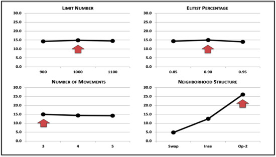
Figure 8.
Parametrization for TSP.
For the TSP, SA will use an initial temperature (Tmax) of 95,000, an epoch length (L) of 4950, a geometric cooling factor (α) of 0.80, Insert as the neighborhood structure and interrupted criterion is 600,000 iterations. For the self-parametrization, the meta-heuristic of the parameters space will use a hive size of 10, a limit number of 50, an elitist percentage of 0.9 and a number of movements of 3. It will be interrupted after 500 iterations. On the other hand, the parameters of the meta-heuristic of the solutions space will be determined automatically, with the exception of the hive size, which will be 30 and the interrupted criterion, which will be 1000 for the TWT and 20,000 for the TSP.
5.2. Results of the Computational Study
For the TWT problem, the conventionally parametrized SA and DABC were run five times, with the best solution reported. For the self-parametrization, each calibration was evaluated in five runs of the meta-heuristic of the solutions space. In this case the min, max and mean values are presented. The results are presented in Table 4.
Table 4.
Results for the TWT Problem.
For the TSP, the results can be examined in Table 5. Once more, the conventionally parametrized SA and DABC were run five times and the best solution is presented. For the self-parametrization, each calibration was evaluated in five runs of the meta-heuristic of the solutions space and the min, max and mean are presented.
Table 5.
Results for the TSP Problem.
In Table 6 computational cost of the conventionally parametrized SA and DABC and the auto-parameterization framework can be analyzed in Table 6 for the TWT problem and in Table 7 for the TSP problem. As expected, the auto-parameterization framework computational cost is much higher than those of the conventionally parametrized SA and DABC, because the auto-parameterization framework performs multiple searches of the solutions space, for each solution of the parameter space, namely, five runs of the meta-heuristic of the solution space for each parameterization solution. It is important to mention that the comparison of the computational cost is not equitable, since time spent in the parameterization cannot be not counted for conventionally parametrized SA and DABC. The difference in the results are reduced when one considers that the parameterization is often a laborious process that requires a considerable know-how and effort by the user.
Table 6.
Computational Cost for the TWT Problem.
Table 7.
Computational Cost for the TSP Problem.
6. Statistical Analyzes
In order to compare the performance of the self-parametrization framework and the conventionally parametrized DABC and SA in the TWT problem and TSP, it is indispensable to normalize the results. For example, a 2134 solution in the first instance of the TWT problem is better than a 2000 solution in the second. Solution from self-parametrization framework and the conventionally parametrized DABC and SA were normalized by the relative deviation to the optimal solution. An alternative would be to normalize by the absolute deviation, but this would not consider the value of the optimal solution. For example, a deviation of 10 is different in a problem where the value of the optimal solution is 2134 or 22. To calculate the relative deviation was used expression (1). F(S)MH represents the solutions of the self-parametrization framework or the conventionally parametrized DABC and SA, and F(S)OTM the optimal solution. Relative deviation to the optimal solution, or when the optimum is unknown, to the best-known solution, is considered the best metric to compare meta-heuristics [76].
6.1. TWT Problem
For the TWT problem the performance of the self-parametrization framework is exceptional, in fact, it presented the user with near optimal solution in all 30 instances. The same was true with the conventionally parametrized DABC, which also found the near optimal solution in all 30 instances. In short, the self-parametrization framework was able to replicate, if not improve on, the conventionally parametrized DABC with complete automatized parametrization procedure. Even the max and mean solutions of the self-parametrization framework are nearly optimal in all instances.
Figure 9 shows the frequency of relative deviation to the optimum of the self-parametrization framework and the conventionally parametrized DABC and SA. It shows the excellent performance of the proposed framework.
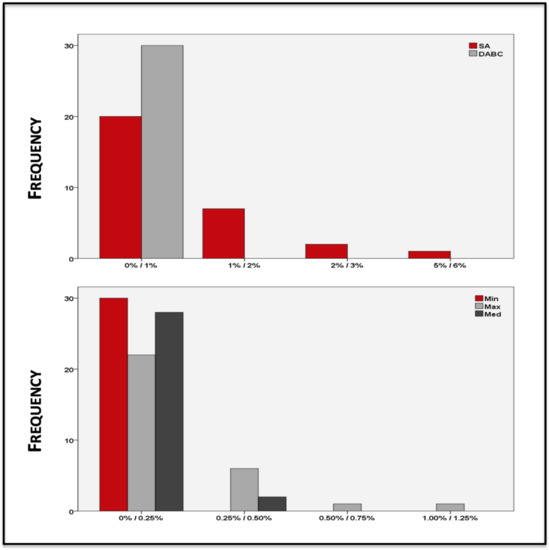
Figure 9.
Relative Deviations for the TWT Problem.
Table 8 shows the values of the mean, median, standard deviation and variance, of the relative deviation to the optimal solution of the self-parametrization framework and the conventionally parametrized DABC and SA. It is clear the proposed framework outperformed the conventionally parametrized DABC.
Table 8.
Statistic of the TWT Problem.
In order to conclude about the performance of the self-parameterization framework, when compared with the conventionally parametrized DABC, a one-way ANOVA (analysis of variance) was used [61]. μMin, μMax and μMed are the mean of the relative deviation from the optimum from the self-parameterization framework and μDABC is the mean of the relative deviation from conventionally parametrized DABC. The ANOVA’s hypotheses are:
- •
- H0:
- •
- H1: Means all not all equal.
In Table 9 it is possible to examine the ANOVA. It found statistical evidence to reject the H0, with 95% confidence. In other words, it is not possible to conclude the performance of the min, max and mean solutions from the self-parameterization framework and the conventionally parametrized DABC are equal (p-Value of 0.000).
Table 9.
ANOVA for TWT Problem.
At least one population did not have an identical performance. In order to identify which, it is necessary to perform the Scheffe test [77]. The Scheffe test is shown in Table 10.
Table 10.
Scheffe Test for TWT Problem.
It is impossible, with 95% confidence, to confirm that the self-parameterization framework performs better than the conventionally parametrized DABC in the TWT problem (p-Value of 0.413). It seems the only difference is between the min and the max solutions of the self-parameterization framework (p-Value of 0.000).
6.2. TSP
In TSP, the self-parametrization framework also outperformed both the conventionally parametrized DABC and SA, but in this case, the disparities between them are noticeable in the examination of Table 5.
Figure 10 shows the frequency of relative deviation to the optimum of the self-parametrization framework and the conventionally parametrized DABC and SA. It shows that proposed framework outperformed DABC and SA.
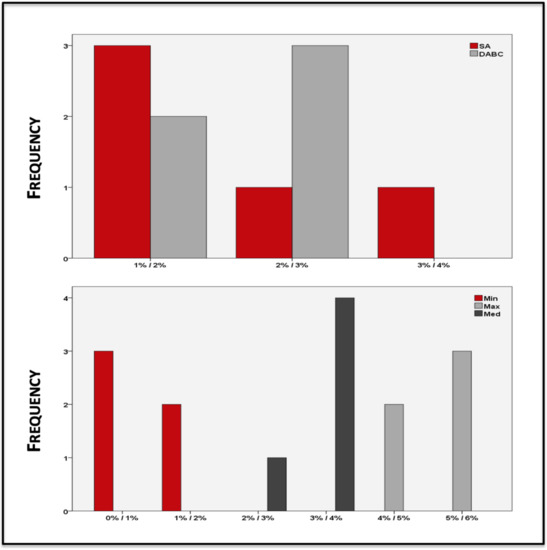
Figure 10.
Relative Deviations for the TSP.
In Table 11 shows the values of the mean, median, standard deviation and variance, of the relative deviation to the optimal solution of the self-parametrization framework and the conventionally parametrized DABC and SA. It is even more obvious the self-parametrization framework outperformed the conventionally parametrized DABC.
Table 11.
Statistic of the TSP.
In order to conclude about the performance of the self-parameterization framework, since it is not possible to assume the normality by the central limit theorem (CLT), it is necessary to use a normality test. The Shapiro–Wilk test will analyze the hypothesis that a sample comes from a normally distributed population when that sample is smaller than 30. Shapiro–Wilk’s hypotheses are:
- •
- H0: The sample is from a population that follows a normal distribution.
- •
- H1: The sample is not from a population that follows a normal distribution.
In Table 12 it possible to examine the Shapiro–Wilk. It found no statistical evidence to discard the H0. In other words, it is not possible to conclude that the sample is not from a normal distributed population (p-value of 0.427).
Table 12.
Shapiro–Wilk for the TSP.
Since it was not possible to demonstrate that the sample does not come from a normal distributed, the self-parametrization framework and conventionally parametrized DABC will be compared with the Student’s. It compares the means of normal distributions samples [61]. Student’s t-test hypotheses are:
- •
- H0:
- •
- H1:
Table 13 shows the Student’s t-test. It found statistical evidence to reject the H0, with 95% confidence. In other words, it is not possible to assume the performance of the self-parameterization framework and the conventionally parametrized DABC are equal for the TSP (p-value of 0.021). Since the sample points to the better performance of the self-parametrization framework, it is possible to conclude it performs better.
Table 13.
Student’s t-test for the TSP.
Since the Shapiro–Wilk test is unprecise for small samples [78], the results were validated with the Mann–Whitney test. The result of the Mann–Whitney was similar to those shown in Table 13, that is, it is not possible to determine the performance of the solutions of the self-parameterization framework and the conventionally parametrized DABC are equal (p-value of 0.032). Since the sample points to the better performance of the self-parametrization framework, it is possible to conclude it performs better.
In short, the statistical inference showed disparities in the performance of the self-parameterization framework and the conventionally parametrized DABC. Even if the self-parameterization framework presented better solutions in both problems, the smaller size of the instances of the TWT problem, ended up mitigating the variance in performance. Overall, the self-parametrization framework, not only found calibrations of the same quality as those found by conventionally parameterization, it was possible to infer that the performance of the self-parameterization framework is superior to that of conventionally parametrization in the TSP.
7. Conclusions
Meta-heuristics can be described as a compromise between the effectiveness of enumerative techniques and the efficiency of approximate techniques, that is, meta-heuristics are able to find “acceptable” solutions. However, the parametrization procedure cannot be disassociated from their performance It is the parameterization procedure that will adapt the meta-heuristics to the problem, or even to the instance of the problem.
In order to streamline the parameterization and, at the same time, allow more inexperienced users to implement meta-heuristics, a self-parametrization framework was developed. It approaches the parameterization procedure as an optimization problem and finds the parameters without user intervention. It uses two meta-heuristics, a meta-heuristic of the parameter space and a meta-heuristic of the solution space. It is the meta-heuristic of the parameter space that searches for calibrations, which are then evaluated by the meta-heuristic of the solution space. Each calibration is evaluated multiple times in order to overcome the stochastic nature of meta-heuristics.
To evaluate the performance of the self-parameterization framework, it was compared with a conventionally parametrized meta-heuristic in 30 instances of the TWT Problem and in five instances of the TSP. The purpose of the comparison was to see if self-parameterization framework would reproduce the results from a conventionally parametrized meta-heuristic, but it exceeded expectations. It outperformed the conventionally parametrized meta-heuristic in both the TWT problem and in TSP. In the TWT, mean relative deviation from the optimum of the framework was 0.009%, compared to the 0.071% for the conventionally parametrized meta-heuristic. In the TSP instances, the self-parameterization framework also obtained a better mean relative deviation from the optimal solutions, but in this case, the statistical inference showed disparities (p value of 0.016).
Some of the limitations of proposed framework are the increase in the computational cost. Such an increase was predictable and is minimized by the total automatization of the parametrization procedure. Moreover, the self-parameterization framework is limited by the characteristics of the meta-heuristic of the parameter space and will require the discretization of the parameters whenever a discrete meta-heuristic is applied.
Future work should validate the proposed framework and compare it with other search-based and hybrid parameterization techniques presented in literature. However, such comparison should consider that other search-based and hybrid parameterization techniques are often inaccessible to users, while the proposed framework does not require a separate parametrization algorithm and can apply to any meta-heuristic, without much effort. Furthermore, the self-parametrization could be incorporated into a scheduling system. It would be able to adapt the parameters of the meta-heuristic to any change, planned or not, in the production environment.
Author Contributions
Conceptualization: A.S.S., A.M.M. and L.R.V.; methodology: A.S.S., A.M.M. and L.R.V.; software: A.S.S., A.M.M. and L.R.V.; validation: A.S.S., A.M.M. and L.R.V.; formal Analysis: A.S.S., A.M.M. and L.R.V.; investigation: A.S.S., A.M.M. and L.R.V.; writing: A.S.S., A.M.M. and L.R.V.; review and editing: A.S.S., A.M.M. and L.R.V. All authors have read and agreed to the published version of the manuscript.
Funding
This work was supported by national funds through the FCT—Fundação para a Ciência e Tecnologia through the R&D Units Project Scopes: UIDB/00319/2020, and EXPL/EME-SIS/1224/2021.
Institutional Review Board Statement
Not applicable.
Informed Consent Statement
Not applicable.
Data Availability Statement
All the problems and instances used in the computational study are available at: http://people.brunel.ac.uk/~mastjjb/jeb/info.html and https://comopt.ifi.uni-heidelberg.de/software/TSPLIB95/ (accessed on the 22 of November of 2021).
Conflicts of Interest
The authors declare no conflict of interest.
References
- Xhafa, F.; Abraham, A. Metaheuristics for Scheduling in Industrial and Manufacturing Applications. In Studies in Computational Intelligence; Springer: Berlin/Heidelberg, Germany, 2008; Volume 128. [Google Scholar]
- Osman, I.; Laporte, G. Metaheuristics: A Bibliography. Ann. Oper. Res. 1996, 63, 511–623. [Google Scholar] [CrossRef]
- Luke, S. Essential of Metaheuristics, 2nd ed.; Lulu: Morrisville, NC, USA, 2013. [Google Scholar]
- Talbi, E. Meta-Heuristics: From Design to Implementation; Wiley: Hoboken, NJ, USA, 2009. [Google Scholar]
- Blum, C.; Roli, A. Metaheuristics in Combinatorial Optimization: Overview and Conceptual Comparison. ACM Comput. Surv. 2003, 35, 268–308. [Google Scholar] [CrossRef]
- Holland, J.H. Adaptation in Natural and Artificial Systems: And Introduction Analysis with Application to Biology, Control and Artificial Intelligence; University of Michigan Press: Cambridge, MA, USA, 1975. [Google Scholar]
- Kirkpatrick, S.; Gelatt, C.D., Jr.; Vecchi, M.P. Optimization by Simulated Annealing. Science 1983, 220, 671–680. [Google Scholar] [CrossRef] [PubMed]
- Černý, V. A Thermodynamical Approach to the Travelling Salesman Problem: An Efficient Simulated Annealing Algorithm. J. Optim. Theory Appl. 1985, 45, 41–51. [Google Scholar] [CrossRef]
- Glover, F. Future Paths for Integer Programming and Links to Artificial Intelligence. Comput. Oper. Res. 1986, 13, 533–549. [Google Scholar] [CrossRef]
- Feo, T.A.; Resende, M.G.C. A Probabilistic Heuristic for a Computationally Difficult Set Covering Problem. Oper. Res. Lett. 1989, 8, 67–77. [Google Scholar] [CrossRef]
- Mladenocić, N.; Hansen, P. Variable Neighborhood Search. Comput. Oper. Res. 1997, 24, 1097–1100. [Google Scholar] [CrossRef]
- Stützle, T.G. Local Search Algorithms for Combinatorial Problems: Analysis, Improvements, and New Applications. Ph.D. Thesis, Department of Computer Science, Darmstadt University of Technology, 64289 Darmstadt, Germany, 1998. [Google Scholar]
- Dorigo, M. Optimization, Learning and Natural Algorithms. Ph.D. Thesis, DEI, Politecnico di Milano, Italy, 1992. [Google Scholar]
- Kennedy, J.; Eberhart, R. Particle Swarm Optimization. In Proceedings of the 1995 IEEE International Conference on Neural Network (ICNN’95), Perth, WA, Australia, 27 November–1 December 1995; pp. 1942–1948. [Google Scholar]
- Passino, K.M. Biomimicry of Bacterial Foraging for Distributed Optimization and Control. IEEE Control. Syst. Mag. 2002, 22, 52–67. [Google Scholar]
- Yang, X.S. Nature-Inspired Metaheuristic Algorithms; Luniver Press: Frome, UK, 2008. [Google Scholar]
- Yang, X.S.; Deb, S. Cuckoo search via Lévy flights. In Proceedings of the 2009 World Congress on Nature & Biologically Inspired Computing (NaBIC 2009), Coimbatore, India, 9–11 December 2009; pp. 210–214. [Google Scholar]
- Yang, X.S. A New Metaheuristic Bat-Inspired Algorithm. In Nature Inspired Cooperative Strategies for Optimization (NISCO 2010); Studies in Computational Intelligence; Springer: Berlin/Heidelberg, Germany, 2016; Volume 284, pp. 65–74. [Google Scholar]
- Mirjalili, S.; Mirjalili, S.M.; Lewis, A. Grey Wolf Optimizer. Adv. Eng. Softw. 2014, 69, 46–61. [Google Scholar] [CrossRef] [Green Version]
- Abed-Alguni, B.H.; Alawad, N.A. Distributed Grey Wolf Optimizer for Scheduling of Workflow Applications in Cloud Environments. Appl. Soft Comput. 2021, 102, 107113. [Google Scholar] [CrossRef]
- Abed-Alguni, B.H.; Alawad, N.A.; Barhoush, M.; Hammed, R. Exploratory cuckoo search for solving single-objective optimization problems. Soft Comput. 2021, 25, 10167–10180. [Google Scholar] [CrossRef]
- Moscato, P. On Evolution, Search, Optimization, Genetic Algorithms and Martial Arts—Towards Memetic Algorithms; Technical Report 826; Caltech Concurrent Computation Program, California Institute of Technology: Pasadena, CA, USA, 1989. [Google Scholar]
- Sörensen, K.; Sevaux, M.; Glover, F. A History of Metaheuristics. In Handbook of Heuristics; Springer: Berlin/Heidelberg, Germany, 2018; pp. 1–8. [Google Scholar]
- Sörensen, K. Metaheuristics: The Metaphor Exposed. Int. Trans. Oper. Res. 2018, 22, 3–18. [Google Scholar] [CrossRef]
- Jung, S.H. Queen-Bee Evolution for Genetic Algorithm. Electron. Lett. 2003, 39, 575–576. [Google Scholar] [CrossRef]
- Abbass, H.A. MBO: Marriage in Honey Bees Optimization—A Haplometrosis Polygynous Swarming Approach. In Proceedings of the 2001 Congress on Evolutionary Computation (CEC), Seoul, Korea, 27–30 May 2001; pp. 207–214. [Google Scholar]
- Lučić, P.; Teodorović, D. Computing with Bees: Attacking Complex Transportation Engineering Problems. Int. J. Artif. Intell. Tools 2003, 12, 375–394. [Google Scholar] [CrossRef]
- Yang, X.S. Engineering Optimization via Nature-Inspired Virtual Bee Algorithms. In Artificial Intelligence and Knowledge Engineering Applications: A Bioinspired Approach; Lecture Notes in Computer Science; Springer: Berlin/Heidelberg, Germany, 2005; Volume 3562, pp. 317–323. [Google Scholar]
- Boussaï, I.; Lepagnot, J.; Siarry, P. A Survey on Optimization Metaheuristics. Inf. Sci. 2013, 237, 82–117. [Google Scholar] [CrossRef]
- Karaboga, D. An Idea Based on Honey Bee Swarm for Numerical Optimization; Technical Report TR06, 2005; Erciyes University, Engineering Faculty, Computer Engineering Department: Kayseri, Turkey, 2005. [Google Scholar]
- Pham, D.T.; Ghanbarzadeh, A.; Koc, E.; Otri, S.; Rahim, S.; Zaidi, M. 2005. Bee Algorithm: A Novel Approach to Function Optimisation; Technical Note: MEC 0501; Cardiff University, The Manufacturing Engineering Center: Cardiff, UK, 2005. [Google Scholar]
- Karaboga, D.; Gorkemli, B. A Combinatorial Artificial Bee Colony Algorithm for Traveling Salesman Problem. In Proceedings of the 2011 International Symposium on Innovations in Intelligent Systems and Applications (INISTA), Istanbul, Turkey, 15–18 June 2011; pp. 50–53. [Google Scholar]
- Liu, Y.; Liu, S. A Hybrid Discrete Artificial Bee Colony Algorithm for Permutation Flowshop Scheduling Problem. Appl. Soft Comput. 2013, 13, 1459–1463. [Google Scholar] [CrossRef]
- Pan, Q.; Tasgetiren, M.F.; Suganthan, P.N.; Chua, T.J. 2011. A Discrete Artificial Bee Colony Algorithm for the Lot-Streaming Flow Shop Scheduling Problem. Inf. Sci. 2011, 181, 2455–2468. [Google Scholar] [CrossRef]
- Shyam Sunder, S.; Suganthan, P.N.; Jin, C.T.; Xiang, C.T.; Soon, C.C. A Hybrid Artificial Bee Colony Algorithm for the Job-Shop Scheduling Problem with No-Wait Constraint. Soft Comput. 2017, 21, 1193–1202. [Google Scholar] [CrossRef]
- Choong, S.S.; Wong, L.; Lim, C.P. An Artificial Bee Colony Algorithm with a Modified Choice Function for the Traveling Salesman Problem. In Proceedings of the 2011 IEEE International Conference on Systems, Man and Cybernetics (SMC), Anchorage, AK, USA, 9–12 October 2011; pp. 357–362. [Google Scholar]
- Soto, R.; Crawford, B.; Vásquez, L.; Zulantay, R.; Jaime, A.; Ramírez, M.; Almonacid, B. Solving the Manufacturing Cell Design Problem Using the Artificial Bee Colony Algorithm. In Multi-Disciplinary Trends in Artificial Intelligence, Lecture Notes in Computer Science; Springer: Cham, Switzerland, 2017; Volume 10607, pp. 473–484. [Google Scholar]
- Santos, A.S.; Madureira, A.M.; Varela, M.R. Evaluation of the Simulated Annealing and the Discrete Artificial Bee Colony in the Weight Tardiness Problem with Taguchi Experiments Parameterization. In Intelligent Systems Design and Applications, Advances in Intelligent Systems and Computing; Springer: Cham, Switzerland, 2017; Volume 557, pp. 718–727. [Google Scholar]
- Hutter, F.; Hoss, H.H.; Stützle, T. Automatic Algorithm Configuration Based on Local Search. In Proceedings of the 2nd National Conference on Artificial Intelligence, Vancouver, BC, Canada, 22–26 July 2007; pp. 1152–1157. [Google Scholar]
- Eiben, A.E.; Hinterding, R.; Michalewicz, Z. Parameter Control in Evolutionary Algorithms. IEEE Trans. Evol. Comput. 1999, 3, 124–141. [Google Scholar] [CrossRef] [Green Version]
- Johnson, D.S. A Theoretician’s Guide to the Experimental Analysis of Algorithms. Available online: https://web.cs.dal.ca/~eem/gradResources/A-theoreticians-guide-to-experimental-analysis-of-algorithms-2001.pdf (accessed on 22 November 2021).
- Montero, E.; Riff, M.C.; Neveu, B. A Beginner’s Guide to Tuning Methods. Appl. Soft Comput. 2014, 17, 39–51. [Google Scholar] [CrossRef]
- Eiben, G.; Schut, M.C. New Ways to Calibrate Evolutionary Algorithms. In Advances in Metaheuristics for Hard Optimization; Springer: Berlin/Heidelberg, Germany, 2007; pp. 153–177. [Google Scholar]
- Lye, L.M. Tools and Toys for Teaching Design of Experiments Methodology. In Proceedings of the 33rd Annual General Conference of the Canadian Society for Civil Engineering, Toronto, ON, Canada, 2–4 June 2005. [Google Scholar]
- Montgomery, D.G. Design and Analysis of Experiments, 6th ed.; John Wiley & Sons: Hoboken, NJ, USA, 2005. [Google Scholar]
- Tanco, M.; Viles, E.; Pozueta, L. Comparing Different Approaches for Design of Experiments (DOE). In Advances in Electrical Engineering and Computational Science, Lecture Notes in Electrical Engineering; Springer: Berlin/Heidelberg, Germany, 2009; Volume 39, pp. 611–621. [Google Scholar]
- Hinkelmann, K. History and Overview of Design and Analysis of Experiments. In Handbook of Design and Analysis of Experiments; Chapman and Hall/CRC: New York, NY, USA, 2015; pp. 3–62. [Google Scholar]
- Box, G.E.P.; Wilson, K.B. On Experimental Attainment of Optimum Conditions. J. R. Stat. Soc. Ser. B 1951, 13, 1–45. [Google Scholar] [CrossRef]
- Roy, R.K. Design of Experiments Using the Taguchi Approach: 16 Steps to Product and Process Improvement; Wiley: New York, NY, USA, 2001. [Google Scholar]
- Durakovic, B. Design of Experiments Application, Concepts, Examples: State of the Art. Period. Eng. Nat. Sci. 2017, 5, 421–439. [Google Scholar] [CrossRef]
- Birattari, M.; Stützle, T.; Paquete, L.; Varrentrapp, K. A Racing Algorithm for Configuring Metaheuristics. In Proceedings of the 4th Annual Conference on Genetic and Evolutionary Computation (GECCO’02), New York, NY, USA, 9–13 July 2002; pp. 11–18. [Google Scholar]
- Hoeffding, W. Probability Inequalities for Sum of Bounded Random Variables. J. Am. Stat. Assoc. 1963, 58, 13–30. [Google Scholar] [CrossRef]
- Montero, E.; Riff, M.C.; Neveu, B. New Requirements for Off-Line Parameter Calibration Algorithms. In Proceedings of the 2010 IEEE Congress on Evolutionary Computation (CEC 2010), Barcelona, Spain, 18–23 July 2010; pp. 1–8. [Google Scholar]
- Balaprakash, P.; Birattari, M.; Stützle, T. Improvement Strategies for the F-Race Algorithm: Sampling Design and Iterative Refinement. In Hybrid Metaheuristics, Lecture Notes in Computer Science; Springer: Berlin/Heidelberg, Germany, 2007; Volume 4771, pp. 108–122. [Google Scholar]
- Bartz-Beislstein, T.; Lasarczyk, C.W.G.; Preuss, M. Sequential Parameter Optimization. In Proceedings of the 2005 IEEE Congress on Evolutionary Computation (CEC 2005), Edinburgh, Scotland, 2–5 September 2005; pp. 773–780. [Google Scholar]
- Mckay, M.D.; Beckman, R.J.; Conover, W.J. A Comparison of Three Methods for Selecting Values of Input Variables in the Analysis of Output from a Computer Code. Technometrics 1979, 21, 239–245. [Google Scholar]
- Huang, D.; Allen, T.T.; Notz, W.I.; Zeng, N. Global Optimization of Stochastic Black-Box Systems via Sequential Kriging Meta-Models. J. Glob. Optim. 2006, 34, 441–466. [Google Scholar] [CrossRef]
- Hutter, F.; Hoos, H.H.; Leyton-Brown, K.; Murphy, K.P. An Experimental Investigation of Model-Based Parameter Optimisation: SPO and Beyond. In Proceedings of the 11th Annual Conference on Genetic and Evolutionary Computation (GECCO’09), Montreal, QC, Canada, 8–12 July 2009; pp. 271–278. [Google Scholar]
- Pereira, I.; Madureira, A.; Costa e Silva, E.; Abraham, A. A Hybrid Metaheuristics Parameter Tuning Approach for Scheduling through Racing and Case-Based Reasoning. Appl. Sci. 2021, 11, 3325. [Google Scholar] [CrossRef]
- Pereira, I.; Madureira, A.; Cunha, B. Metaheuristics Parameter Tuning using Racing and Case-based Reasoning. In Intelligent Systems Design and Applications, Advances in Intelligent Systems and Computing; Springer: Cham, Switzerland, 2017; Volume 557, pp. 911–920. [Google Scholar]
- Pereira, I.; Madureira, A. Self-Optimizing A Multi-Agent Scheduling System: A Racing Based Approach. In Intelligent Distributed Computing IX. Studies in Computational Intelligence; Springer: Cham, Switzerland, 2016; Volume 616, pp. 275–284. [Google Scholar]
- Pereira, I.; Madureira, A.; Moura Oliveira, P.; Abraham, A. Tuning Meta-Heuristics Using Multi-Agent Learning in a Scheduling System. In LNCS Transactions on Computational Science; Springer: Berlin/Heidelberg, Germany, 2013. [Google Scholar]
- Madureira, A.; Pereira, I.; Falcão, D. Cooperative Scheduling System with Emergent Swarm Based Behavior. In Information Systems and Technologies, Advances in Intelligent Systems and Computing; Springer: Berlin/Heidelberg, Germany, 2013; Volume 206, pp. 661–671. [Google Scholar]
- Pereira, I.; Madureira, A.; Moura Oliveira, P. Meta-heuristics Self-Parameterization in a Multi-agent Scheduling System Using Case-Based Reasoning. In Computational Intelligence and Decision Making—Trends and Applications, Intelligent Systems, Control and Automation: Science and Engineering; Springer: Berlin/Heidelberg, Germany, 2013; Volume 61, pp. 99–109. [Google Scholar]
- Grefenstette, J.J. Optimization of Control Parameters for Genetic Algorithms. IEEE Trans. Syst. Man Cybern. 1986, 16, 122–128. [Google Scholar] [CrossRef]
- Nannen, V.; Eiben, A.E. Relevance Estimation and Value Calibration of Evolutionary Algorithm Parameters. In Proceedings of the 20th International Joint Conference on Artificial Intelligence (IJCAI), Hyderabad, India, 6–12 January 2007; pp. 1034–1039. [Google Scholar]
- Nannen, V.; Eiben, A.E. Efficient Relevance Estimation and Value Calibration of Evolutionary Algorithm Parameters. In Proceedings of the 2007 IEEE Congress on Evolutionary Computation, Singapore, 25–28 September 2007; pp. 103–110. [Google Scholar]
- Adenso-Díaz, B.; Laguna, M. Fine-Tuning of Algorithms Using Fractional Experimental Designs and Local Search. Oper. Res. 2006, 54, 99–144. [Google Scholar] [CrossRef]
- Beasley, J.E. ORLibrary. 1990. Available online: http://people.brunel.ac.uk/~mastjjb/jeb/info.html (accessed on 22 November 2021).
- Reinelt, G. TSPLIB. 1991. Available online: https://comopt.ifi.uni-heidelberg.de/software/TSPLIB95/ (accessed on 22 November 2021).
- Anily, S.; Federgruen, A. Simulated Annealing Methods with General Acceptance Probabilities. J. Appl. Probab. 1987, 24, 657–667. [Google Scholar] [CrossRef] [Green Version]
- Park, M.W.; Kim, Y.D. A Systematic Procedure for Setting Parameters in Simulated Annealing Algorithms. Comput. Oper. Res. 1998, 25, 207–217. [Google Scholar] [CrossRef]
- Santos, A.S.; Madureira, A.M.; Varela, M.L.R. The Influence of Problem Specific Neighborhood Structures in Metaheuristics Performance. J. Math. 2018, 2018, 8072621. [Google Scholar] [CrossRef]
- Kiran, M.S.; Gündüz, M. The Analysis of Peculiar Control Parameters of Artificial Bee Colony Algorithm on the Numerical Optimization Problems. J. Comput. Commun. 2014, 2, 127–136. [Google Scholar] [CrossRef]
- Akay, B.; Karaboga, D. Parameter Tuning for the Artificial Bee Colony Algorithm. In Computational Collective Intelligence: Semantics Web, Social Networks and Multiagent Systems, Lecture Notes in Computer Science; Springer: Berlin/Heidelberg, Germany, 2009; Volume 5796, pp. 608–619. [Google Scholar]
- Silberholz, J.; Golden, B. Comparison of Metaheuristics. In Handbook of Metaheuristics; International Series in Operation Research & Management Sciences Springer: Berlin/Heidelberg, Germany, 2010; Volume 146, pp. 625–640. [Google Scholar]
- Ross, S.M. Introductory Statistics, 4th ed.; Elsevier Science, Academic Press: Cambridge, MA, USA, 2017. [Google Scholar]
- Rochon, J.; Gondan, M.; Kieser, M. To Test or Not to Test: Preliminary Assessment of Normality when Comparing Two Independent Samples. BMC Med. Res. Methodol. 2012, 12, 81. [Google Scholar] [CrossRef] [PubMed] [Green Version]
Publisher’s Note: MDPI stays neutral with regard to jurisdictional claims in published maps and institutional affiliations. |
© 2022 by the authors. Licensee MDPI, Basel, Switzerland. This article is an open access article distributed under the terms and conditions of the Creative Commons Attribution (CC BY) license (https://creativecommons.org/licenses/by/4.0/).