Article

Novel Photovoltaic Empirical Mathematical Model Based on Function Representation of Captured Figures from Commercial Panels Datasheet

1
Basic and Applied Science Department, College of Engineering and Technology, Arab Academy for Science and Technology (AAST), Smart Village Campus, Giza 12577, Egypt
2
Electrical Engineering Department, College of Engineering and Technology, Arab Academy for Science and Technology (AAST), Abo Kir Campus, Alexandria 1029, Egypt
*
Author to whom correspondence should be addressed.
Mathematics 2022, 10(3), 476; https://doi.org/10.3390/math10030476
Submission received: 30 November 2021 / Revised: 24 December 2021 / Accepted: 15 January 2022 / Published: 1 February 2022
(This article belongs to the Special Issue Mathematics and Its Applications in Science and Engineering)

Abstract

:
Photovoltaic (PV) technology is gaining much interest as a clean, sustainable, noise-free source of energy. However, the non-linear behavior of PV modules and their dependency on varying environmental conditions require thorough study and analysis. Many PV modeling techniques have been introduced in the literature, yet they exhibit several complexity levels for parameter extraction and constants estimation for PV power forecast. Comparatively, a simple, accurate, fast, and user friendly PV modeling technique is proposed in this paper featuring the least computational time and effort. Based on function representation of PV curves’ available in PV datasheets, an empirical mathematical equation is derived. The proposed formula is considered a generic tool capable of modeling any PV device under various weather conditions without either parameter estimation nor power prediction. The proposed model is validated using experimental data of commercial PV panels’ manufacturers under various environmental conditions for different power levels. The obtained results verified the effectiveness of the proposed PV model.

1. Introduction

With the increasing world-wide demand for renewable energy resources, photovoltaic (PV) systems are gaining much interest. Hence, advances are continuously carried out in the field of their modeling and performance [1]. A PV system includes a PV power source in the form of series and/or parallel combinations of PV modules forming a PV array with the required voltage and amperage [
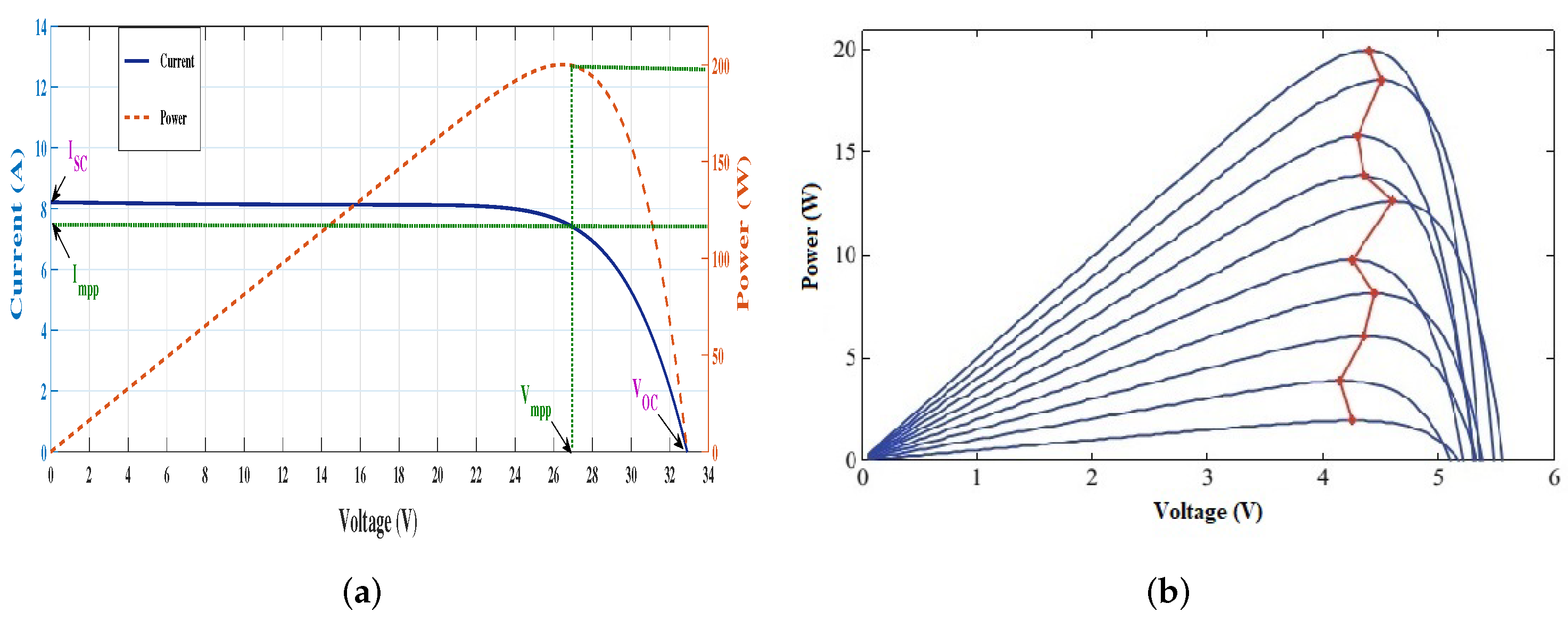
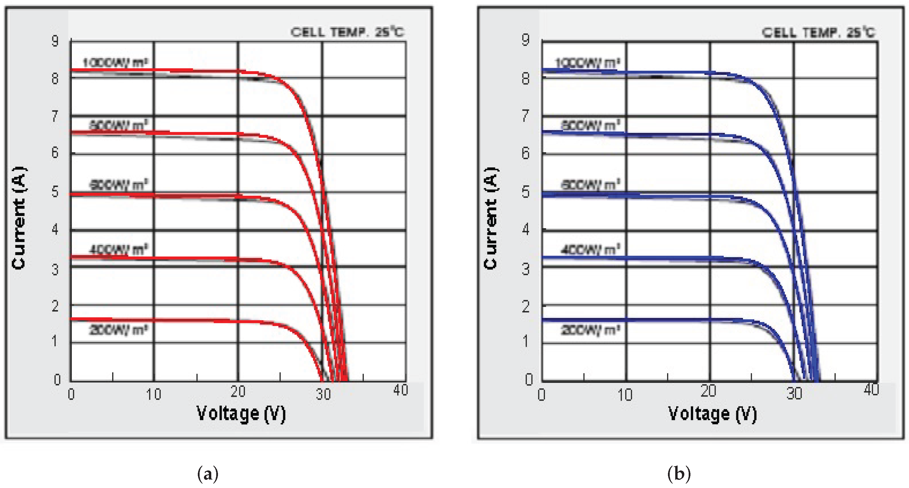
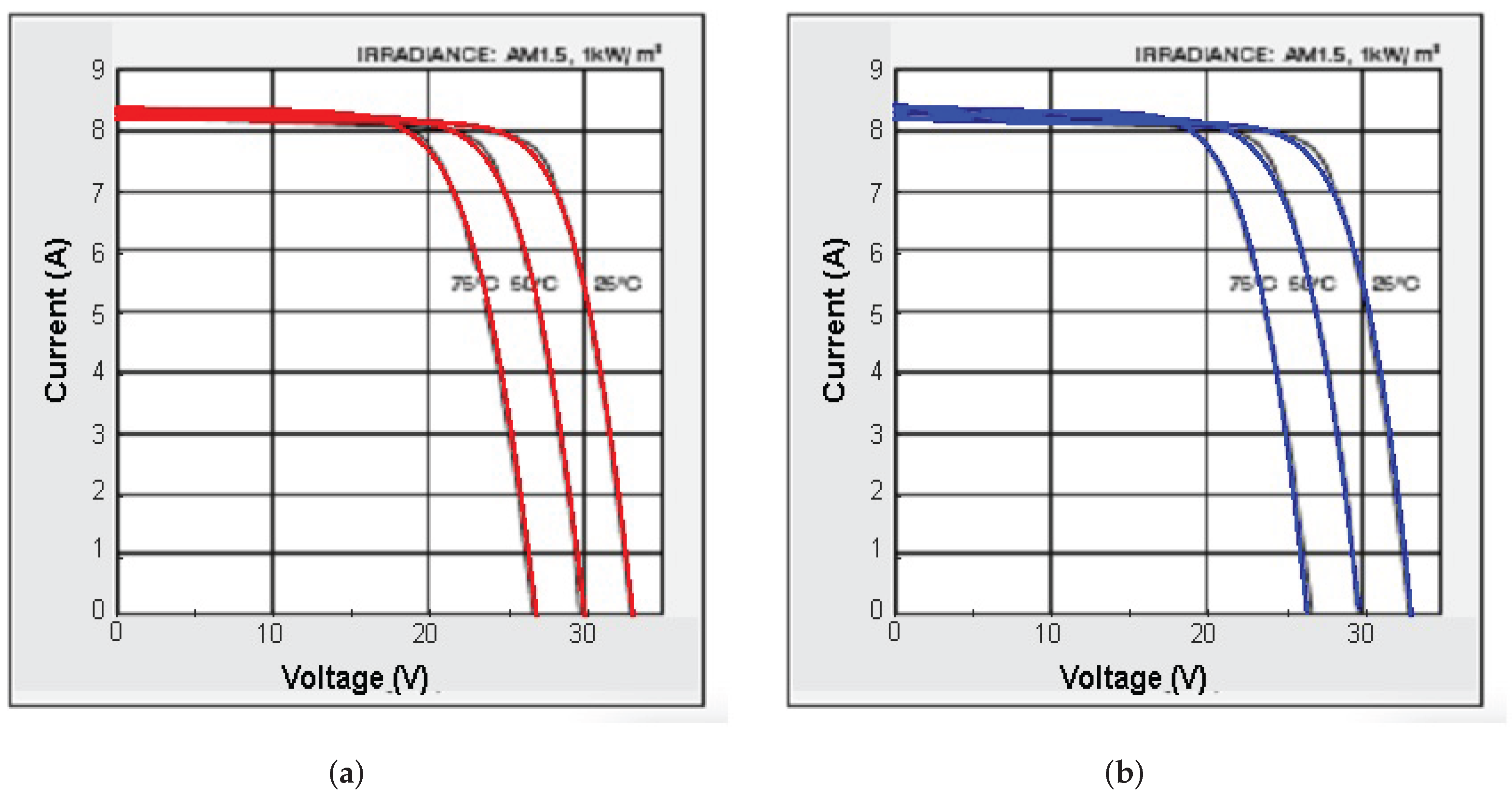
2]. Under uniform environmental conditions, a PV module exerts non-linear electrical characteristic curves, as shown in Figure 1a, where the PV module gives its maximum possible output power at a certain operating point. This maximum power point (MPP) is irradiance and temperature dependent, as presented in Figure 1b [3]. In order to maximize the PV source efficiency under varying environmental conditions, it should be followed by a pulse width modulation (PWM) converter for continuous maximum power point tracking (MPPT) [4].
For robust control of the entire PV system operation, the PV device should be simulated in the virtual environment [5]. Thus, a simple, reliable and precise mathematical model of the PV source is mandatory for accurate analysis of its non-linear characteristics under varying conditions. An efficient PV model is useful in the prediction of PV output power, the analysis of PV converter dynamic behavior and the study of MPP tracking algorithms [6]. PV model accuracy is evaluated by the proximity of the model characteristics to that of the practical device experimental data. Hence, the model should be adjusted using the set of data provided by manufacturers regarding the PV module thermal and electrical characteristics.
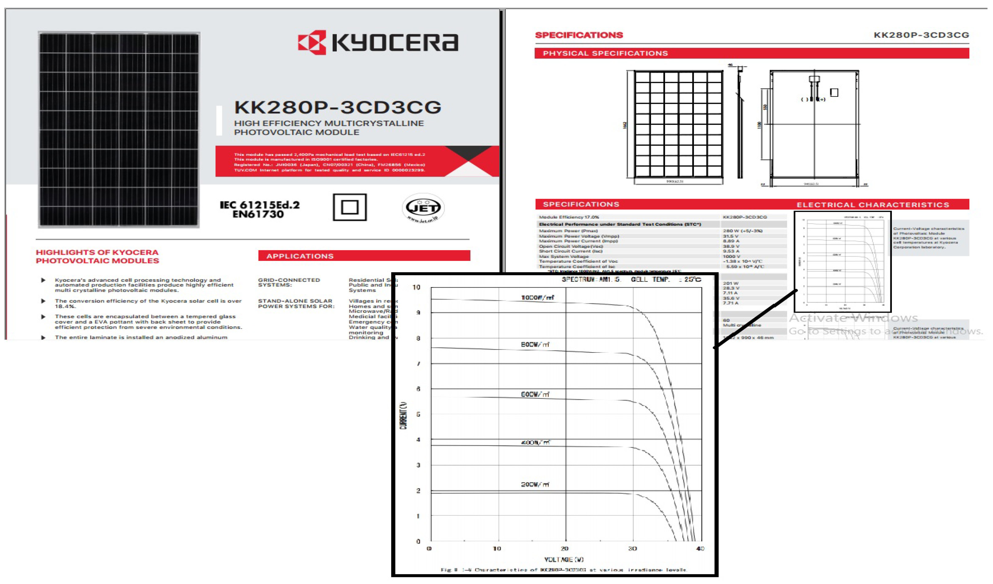
However, PV datasheets present a few experimental data that include the nominal open-circuit voltage ( V O C ), the nominal short-circuit current ( I S C ), the voltage at the MPP ( V M P P ), the current at the MPP ( I M P P ), the maximum experimental peak output power ( P M P P ), the open-circuit voltage/temperature coefficient ( K V ), and the short circuit current/temperature coefficient ( K I ) [7]. These data are given under the so-called standard test condition (STC) which is defined by irradiation level of 1000 W/m2, cell temperature of 25 °C, and air mass value of 1.5 [8]. Some manufacturers may also provide I–V characteristic curves, obtained experimentally under variable operating conditions, to validate and adjust the derived mathematical model. However, obtaining such curves experimentally requires costly and difficult measurements in controlled environmental chambers that should be carried out under certain conditions and according to a number of guidelines [9].
Many approaches have been developed for PV modules’ modeling and representation as will be illustrated in the following. Equivalent circuit-based PV models, applying the Shockley diode equation for solar cell mathematical representation, have been developed and validated using the experimental data given in manufacturers’ datasheets [10]. This equation represents the non-linear characteristics of the PV cell, yet it includes several parameters that are not available in commercial manufacturers’ datasheets, hence have to be estimated [7,11]. These parameters include the diode ideality factor (a), diode reverse saturation current ( I o ), the light-generated current ( I P V ), and practical PV device series and shunt resistances. The series resistance ( R s ) represents the summation of PV panel structural resistances while the parallel resistance ( R P ) mirrors the p n junction leakage current and depends on the PV cell fabrication method. These unknown parameters differ from one panel to another, thus they should be accurately estimated for correct model adjustment of the considered PV device.
Equivalent circuit-based PV models are either based on single-diode equivalent circuits [12,13,14,15], two-diode circuits [16,17,18,19], or three-diode circuits [20,21]. When more diodes are included in the model, higher accuracy is obtained, though at the cost of more complexity and computational effort as more parameters have to be estimated (i.e., additional ideality factor and reverse saturation current for each added diode) [22,23]. For simplicity, most developed PV models are based on the single-diode equivalent circuit, as this model offers a satisfactory compromise between simplicity and accuracy [11]. Different mathematical procedures for estimating the unknown PV parameters required are elaborated with different levels of implementation complexity, computational time, and accuracy [24,25,26]. These procedures can be analytical, numerical, artificial intelligence-based, evolutionary algorithms-based, or hybrid ones.
Normally, analytical mathematical methods give exact solutions by means of algebraic equations. However, due to PV nonlinearity, it is hard to find out the analytical solution of all unknown parameters. Thus, analytical methods apply approximations or simplified assumptions for some PV parameters resulting in fast and simple solution at the cost of relatively less accuracy [27,28]. Generally, the R P value is high while that of R s is very low, thus some authors neglect the former [29,30,31,32] while others neglect the latter [33,34] or both [35]. In [36,37,38,39,40], an analytical method based on Lambert W function is introduced for parameters extraction, while in [41] transcendental equations for solar cell analysis are presented and solved using Special Tran Function Theory (STFT) to increase estimation accuracy.
Numerical methods develop a set of equations which are solved using numerical or iterative algorithms for precise parameters estimation. In [42], an iterative process is applied where R s is slowly incremented and corresponding R P and I P V values are obtained such that the mathematical I–V equation fits specific experimental points on the practical module I–V curve. In [43], an iterative method to find the actual value of the diode ideality factor is presented. Other methods apply optimization numerical algorithms such as Levenberg–Marquardt Algorithm (LMA), Newton Raphson nonlinear, or least-squares algorithm for best curve fitting [27,44]. Although numerical methods outweigh analytical algorithms regarding accuracy, they require long-term time series data, thus consume more time.
Applying artificial intelligence [45,46,47] and evolutionary techniques [48,49,50,51,52,53] for PV parameters extraction can be observed as a fast and accurate solution, yet one which lacks simplicity and requires more computational effort, making it less practical. Hybrid techniques are introduced to compromise between simplicity, accuracy, and computational time. In [54] a combination between numerical and analytical methods is presented where PV output current expression is determined by Lambert W function while the PV voltage is computed numerically by the Newton–Raphson method. Lambert W function along with artificial neural network were employed for determination of PV I–V and PV curves [55].
Beside the equivalent circuit-based PV modeling techniques, an alternative PV cell mathematical representation based on trigonometrically function (sine and cosine function based model) is presented in [56,57]. It depends on observing how PV short-circuit current and open-circuit voltage change versus irradiance and temperature, then translating this observation into a trigonometrically property. However, this trigonometric function includes seven constants whose values have to be obtained through PV experimental characteristics which, in turn, adds to the computational efforts and affects its practicality.
Recently, many approaches have been developed to build PV models based on short-term and long-term PV power forecast using ANN and machine learning techniques [58,59,60,61,62]. However, they require complicated implementation, a large number of data samples, and continuous training and fitting results for accurate forecasting. The developed PV modules’ modeling approaches and representation can be summarized and listed as shown below:
PV Modeling Approaches:
In this paper, a novel generic PV model is presented featuring an empirical mathematical equation based on function representation of captured figures from the datasheet. This model is able to produce characteristic curves for any PV device at any condition based only on four electrical terms found in any practical PV datasheet at standard testing condition (STC). The proposed approach outweighs other models regarding its simplicity and reduced computational time and effort as none of parameters extraction, constants estimation, or PV power forecast are required. Thus, PV experimental curves at different environmental conditions can be emulated easily with the least cost. The proposed model is tested for different practical PV modules at various power ratings, then compared to a conventional PV model based on a single-diode equivalent circuit. The results validated the proposed approach and verified its competitiveness.
This paper is organized as follows: 
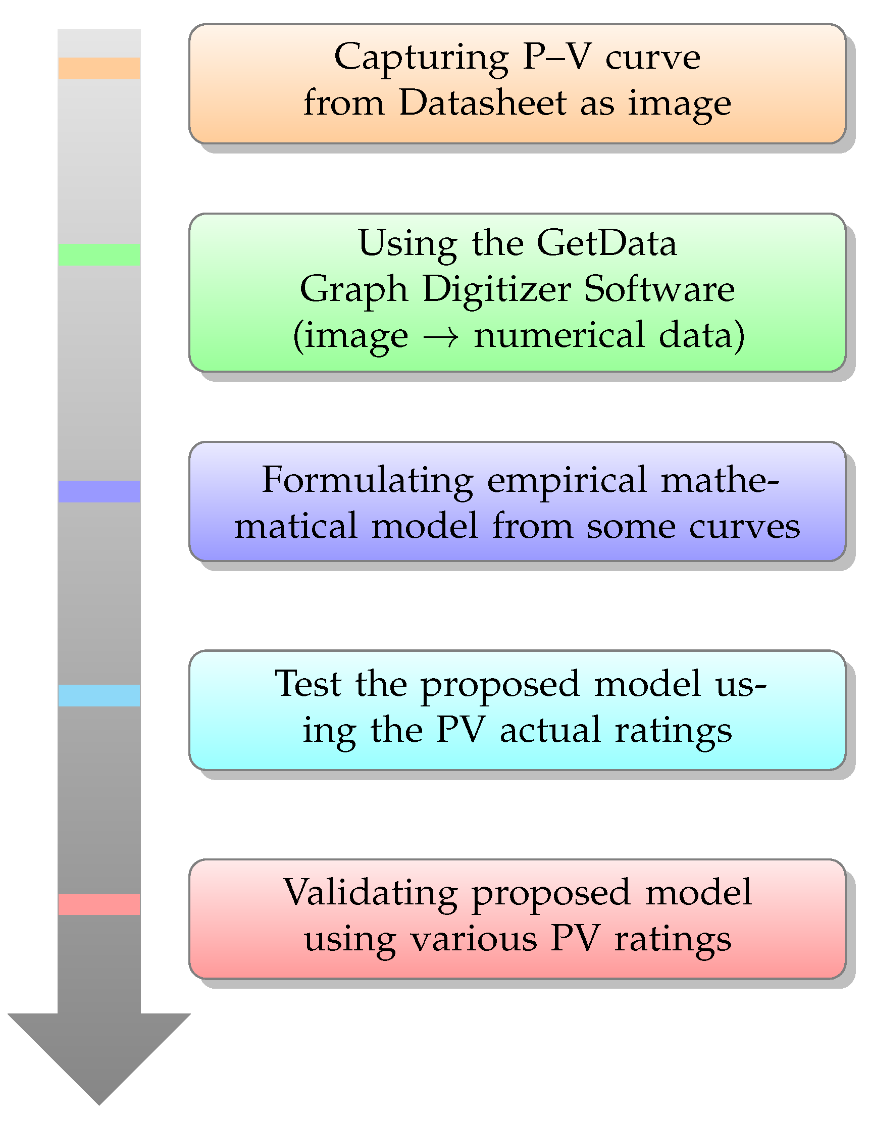
Section 2 illustrates the methodology adopted for developing the proposed empirical mathematical model of the PV based on captured figures from datasheet. 
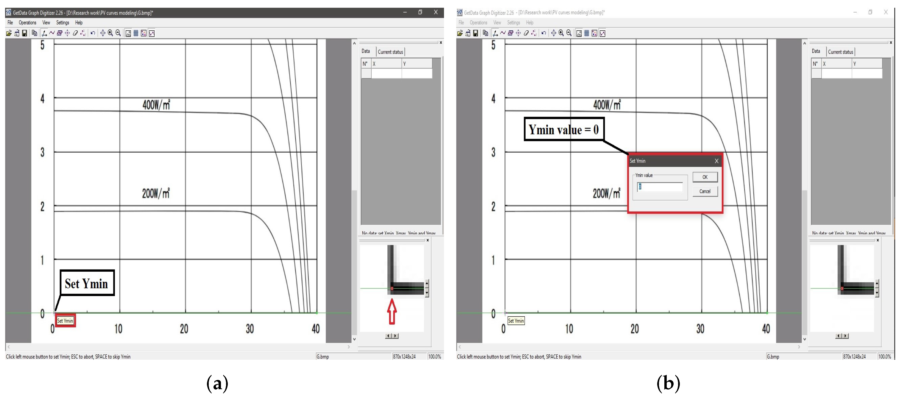
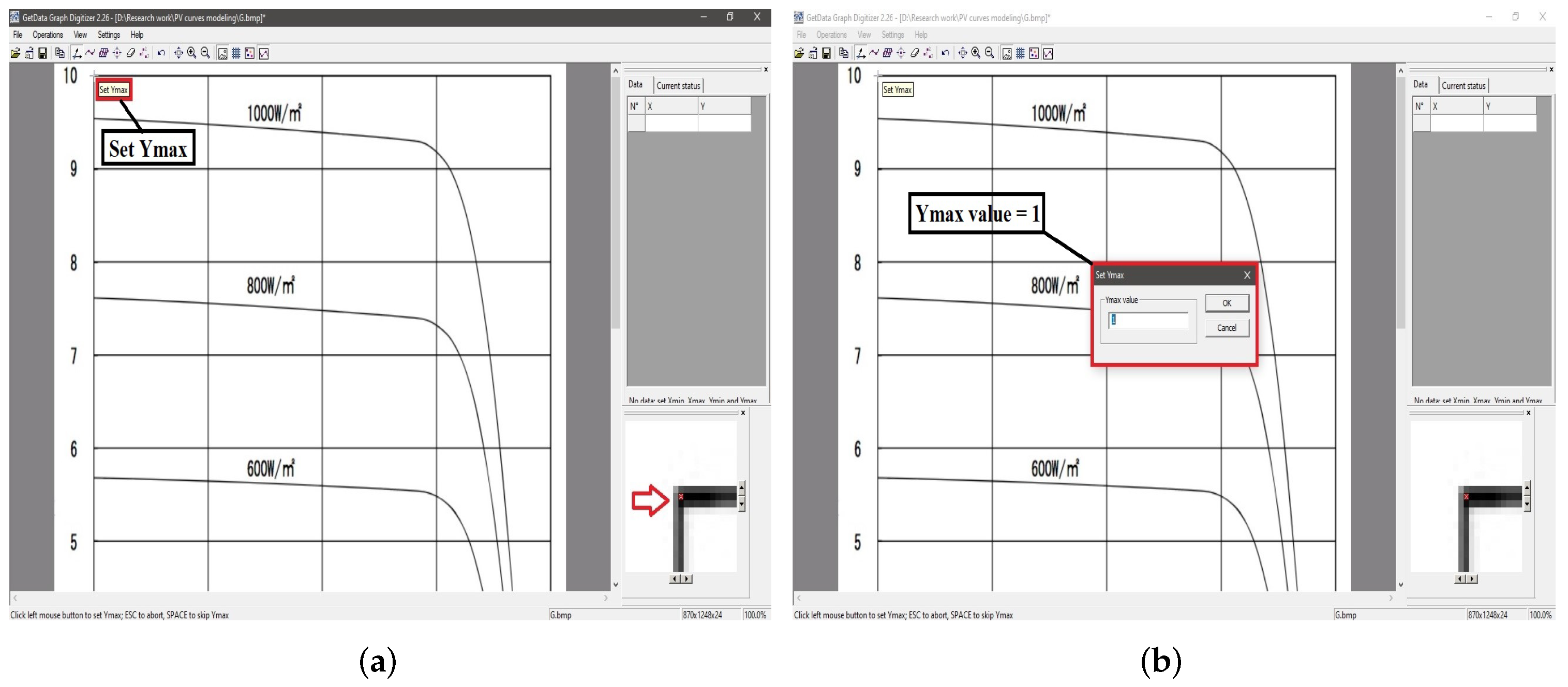
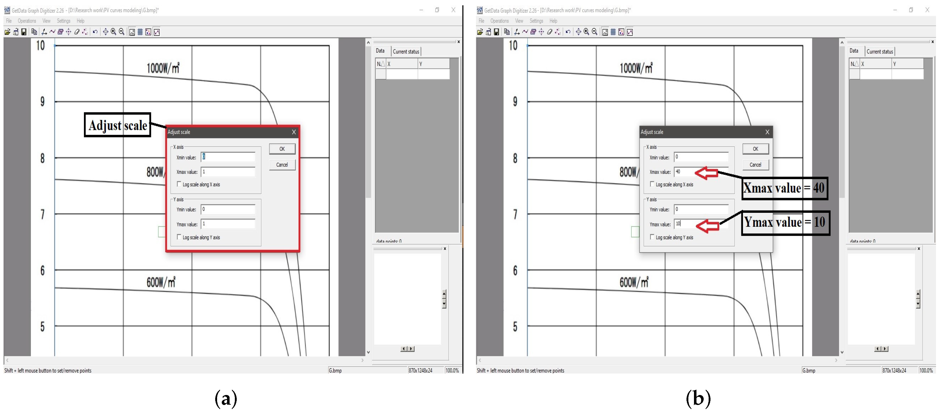
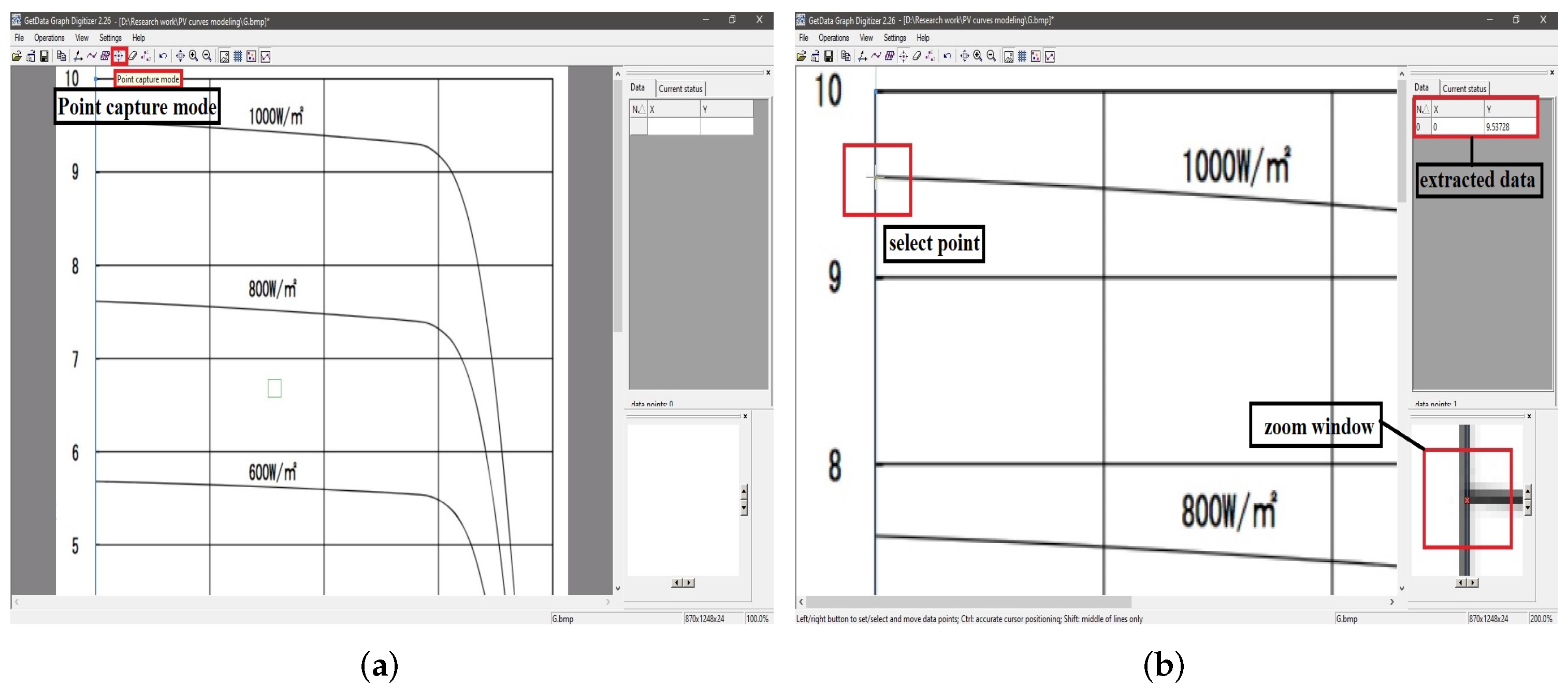
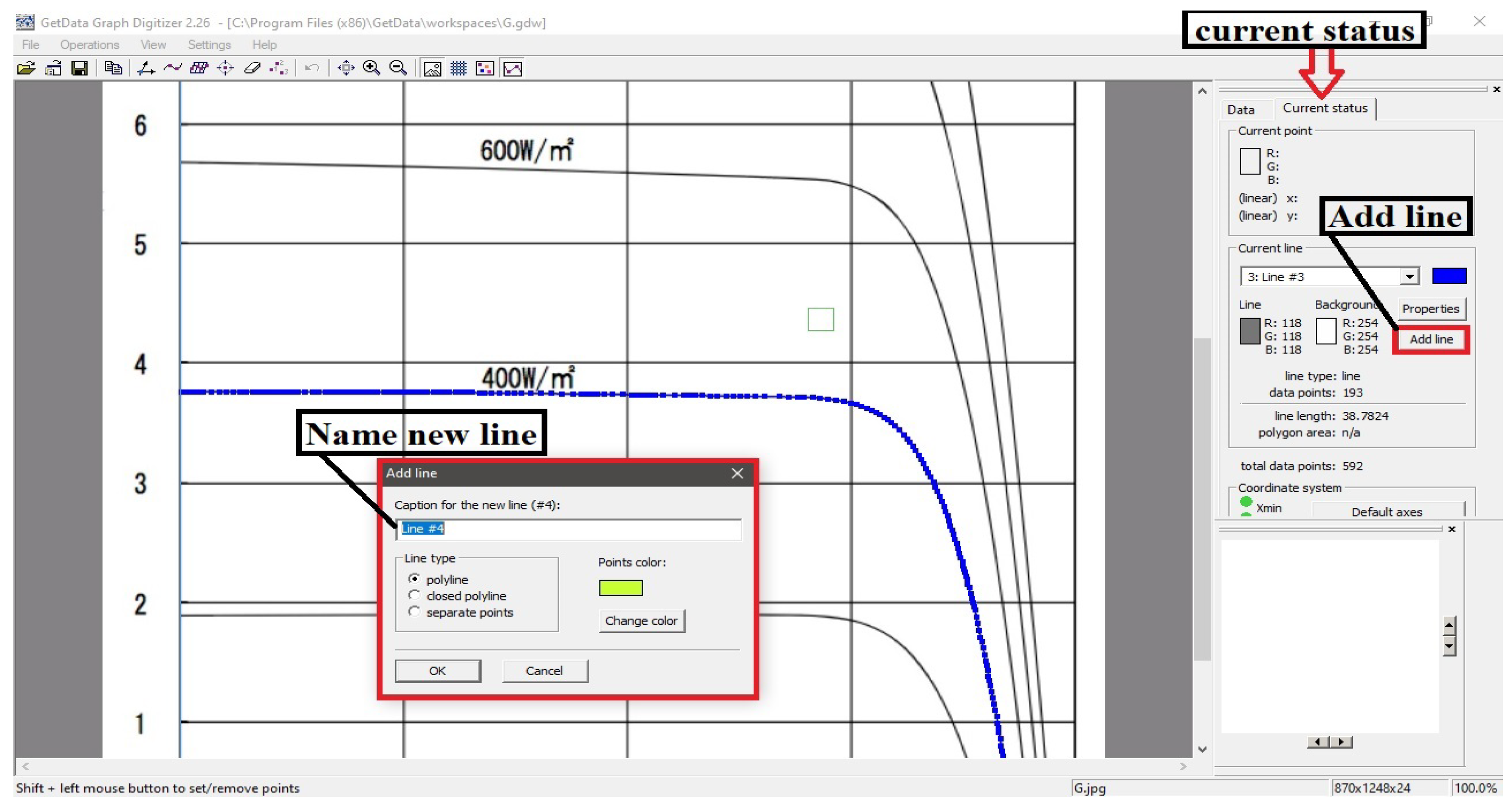
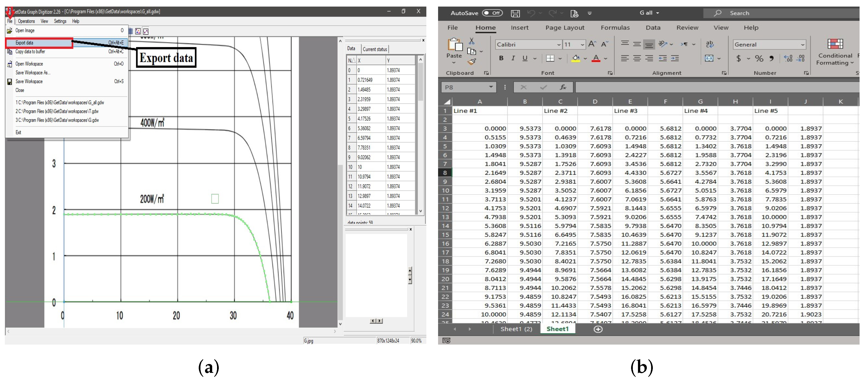
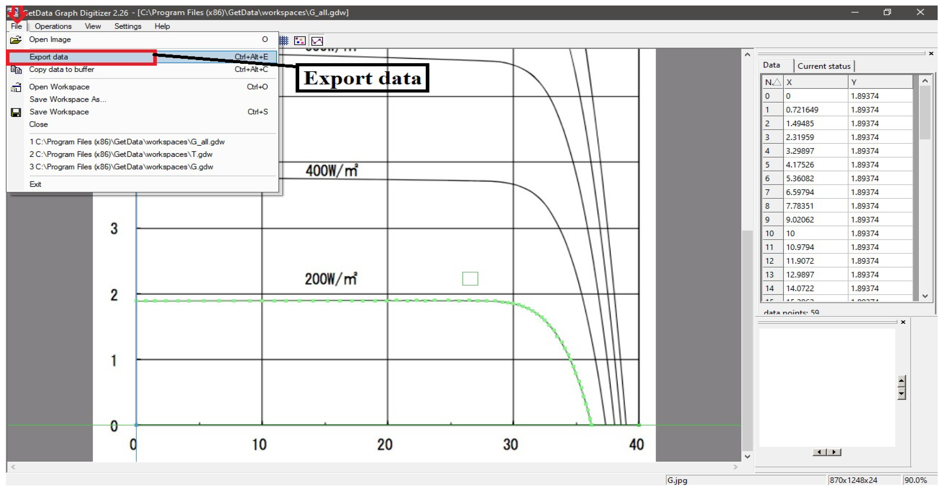
Section 3 includes phase one of the model development of digitizing the captured figures and the data extraction process from the datasheet. Section 4 demonstrates phase two, which presents the formulation of the model through three cases: (i) varying irradiance at fixed STC temperature level, (ii) varying temperature at fixed STC irradiance level, and (iii) specific irradiance and temperature values differ from STC nominal values. 
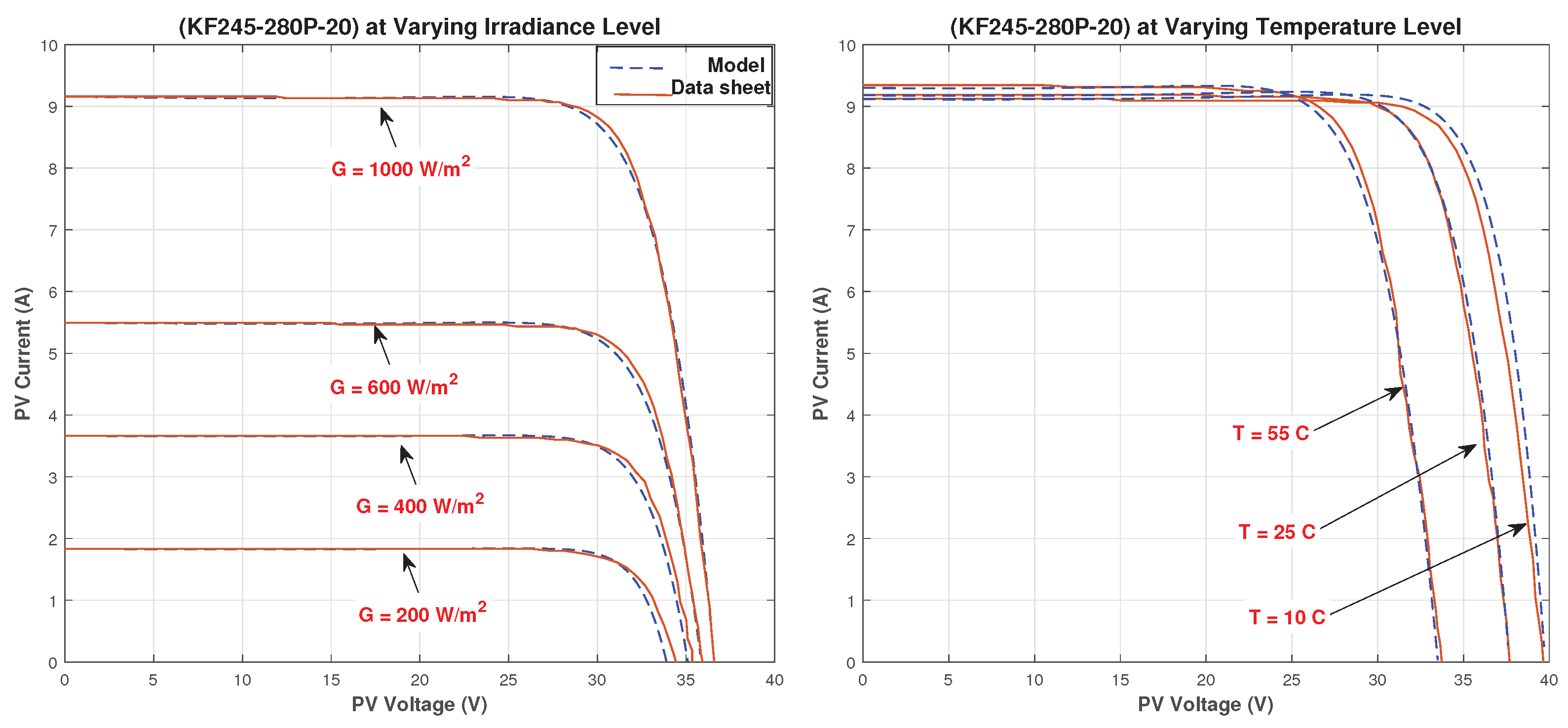
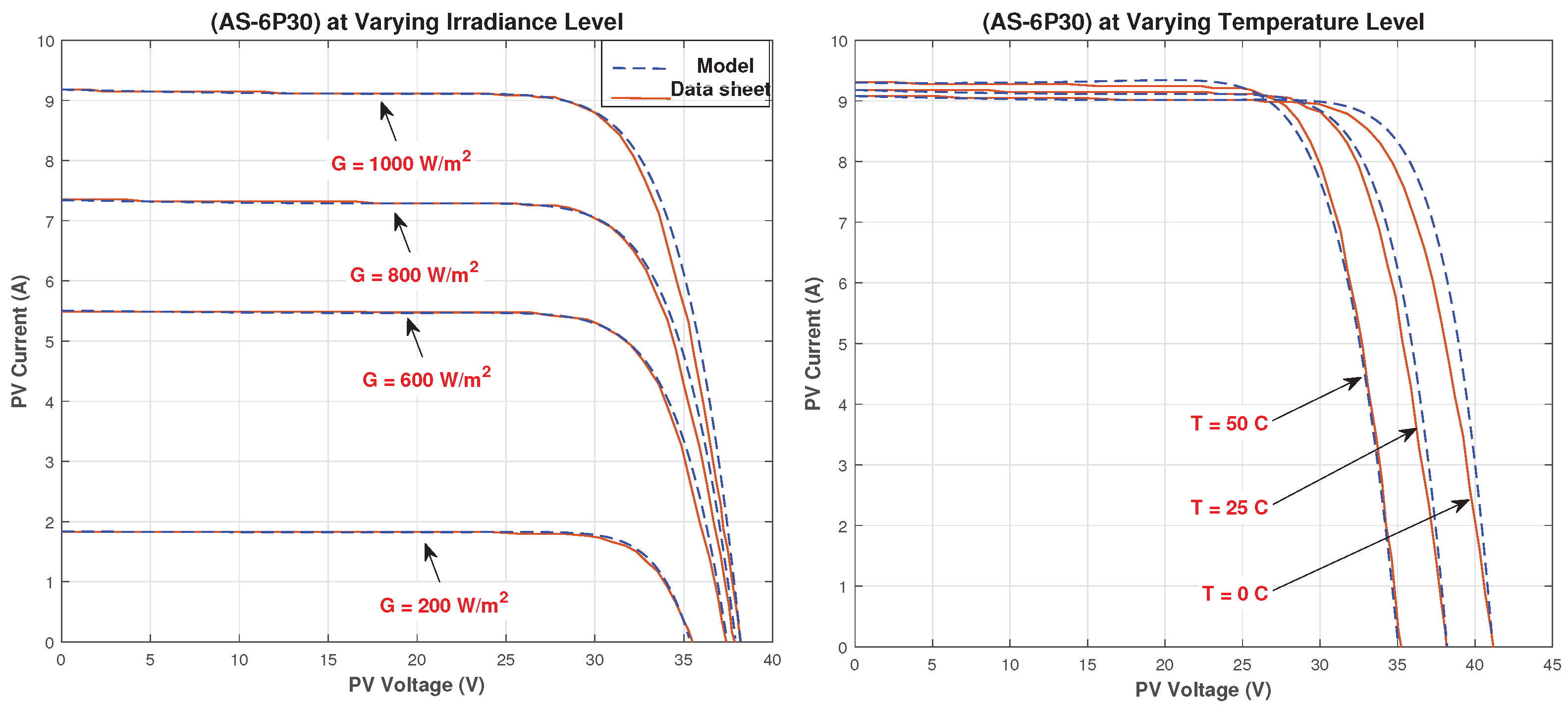
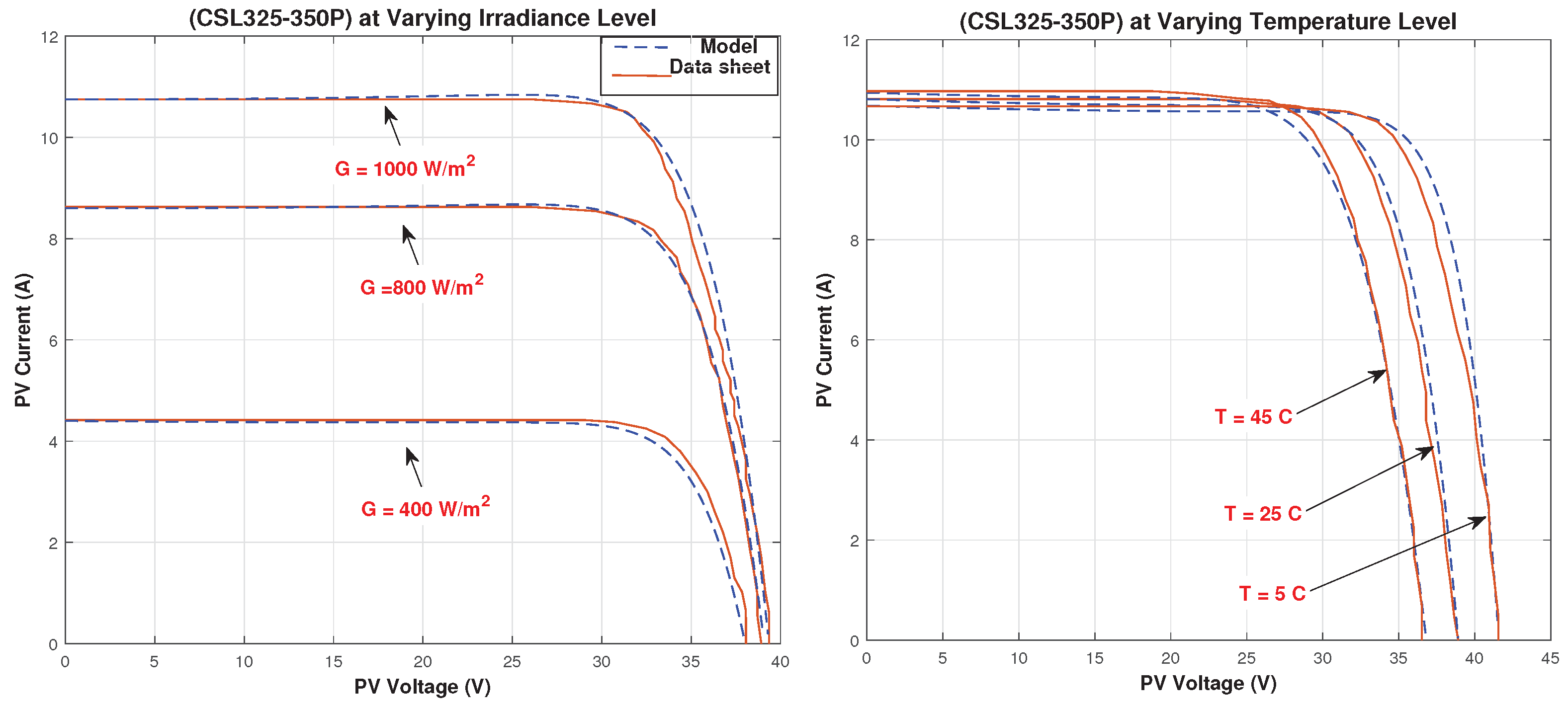
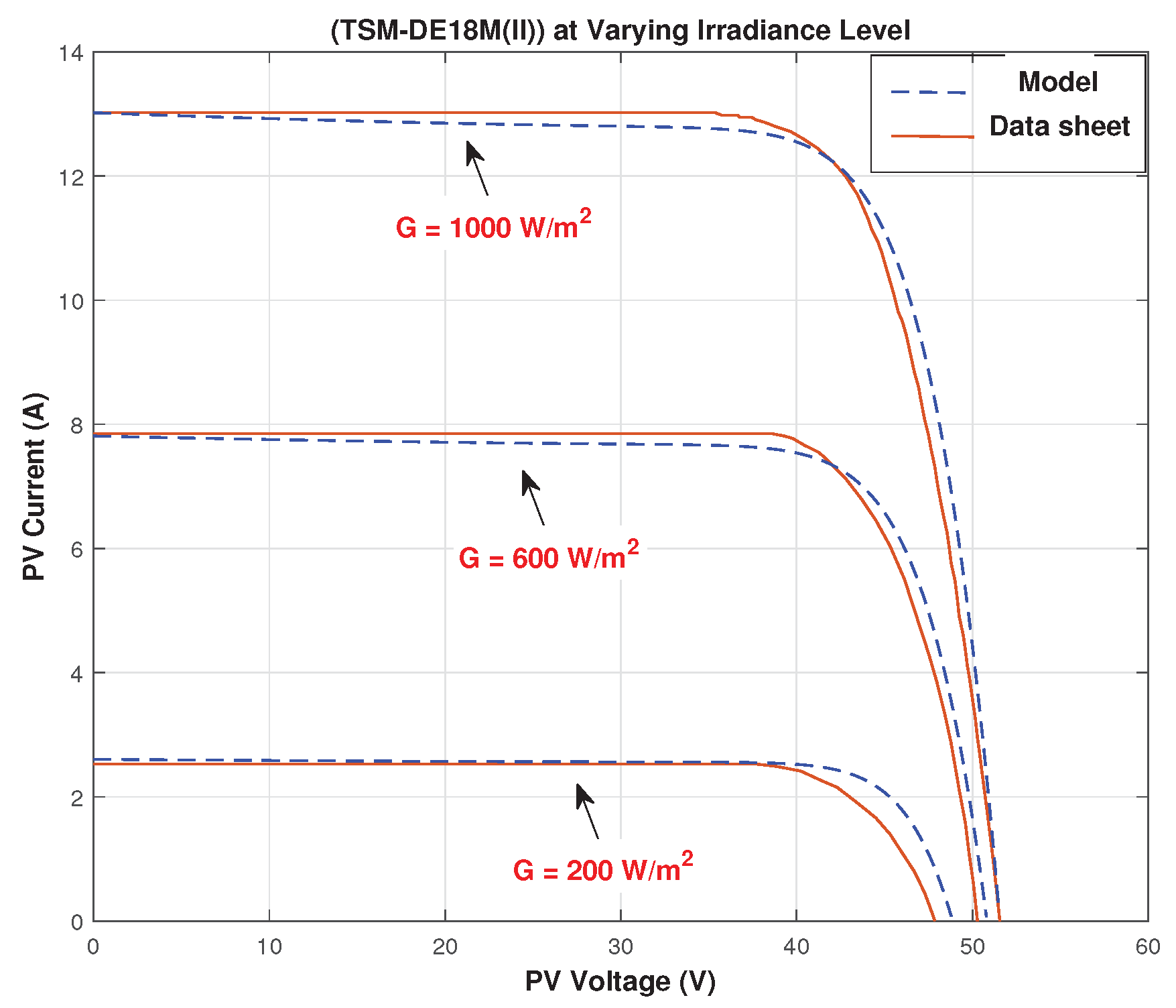
Section 5 includes the simulation results of the proposed model compared to the extracted data. Section 6 contains the model validation using various datasheet with different ratings. Section 7 presents a comparison between the proposed mathematical model and a conventional equivalent circuit based PV model. Finally, Section 8 presents the discussion and conclusion.

2. Methodology of the Proposed Empirical Mathematical Model

The process of developing an empirical mathematical model to be used for generating the characteristic I–V curves of the PV panel at different levels of irradiance and temperatures passes through several steps, represented in Figure 2. In this paper, the proposed methodology is performed using the datasheet of KYOCERA PV-model (KK280P-3CD3CG) [63]. The adopted method for developing an empirical mathematical model starts with capturing the curves as images form the datasheet for the irradiance and temperature variations, as shown in Figure 3. We then used software to digitize these curves by transforming the captured images into numerical data points that are used to analyze the curve features in order to represent them in mathematical functions forms, as shown in Figure 4. By investigating the curves’ characteristics and linking them with the panel standard test condition (STC) the model is developed to represent the I–V curves for the STC irradiance and temperature values (G0 = 1000 W/m2 and T0 = 25 °C). Then, the proposed empirical mathematical model is generalized for any irradiance and/or temperature values based on analyzing the effect of the variation in some of I–V curves in the used main datasheet due to the changing in the values of irradiance and temperature. After that, the remaining unused curves of the same datasheet are used to test the proposed model. To validate the developed empirical model, various data from different panels rating datasheets are used [64,65,66,67]. The following sections will include a detailed illustration of each stage of the proposed methodology.

3. Stage One: Digitizing the Extracted I–V Curves Images from PV Panel Datasheet

In order to study the I–V curves of the PV-panels presented in datasheet, it is first required to transform them into numerical values. Hence, the software GetData Graph Digitizer® is used. This software is based on manually selecting the points from the curves image. At the beginning, one defines the minimum and maximum values of each axis and sets on image and after that defines its scale values. Then, for each curve in the image, the points are selected by tracing the curve using data pointers. These steps are presented in Figure 5.
A zoom preview exists on the bottom right of this program window to increase the accuracy of selecting the points. The data points are stored in Excel sheet format which can be exported to be used in analyzing and validating the mathematical model. This process of data extraction is used for both curves at various irradiance and temperature values.
The following part of this section includes a step-by-step illustration guide of how to use the program in transforming the datasheet I–V curves images into Excel sheet format aided with screen shoots. The data extraction steps are:
  • Import the datasheet curves to the software as image, then start to set the axes points as shown in Figure 6.
  • Set the minimum and maximum points of the x-axis (default 0, 1) as shown in Figure 7 and Figure 8, respectively.
  • Set the minimum and maximum points of the y-axis (default 0, 1) as shown in Figure 9 and Figure 10, respectively.
  • Adjust the scale of the maximum values of the axes based on datasheet values as shown in Figure 11.
  • Extract the data from each curve for a certain irradiance value by moving the selecting cursor along each curve as shown in Figure 12.
  • For adding more than one curve in the data, select add line to start selecting data for the new curve as shown in Figure 13.
  • Export the data from the software as Excel spreadsheet as two columns for each line, representing x and y values for each pair of points, as shown in Figure 14.

4. Stage Two: The Proposed Empirical Mathematical Model of PV Characteristics Curves

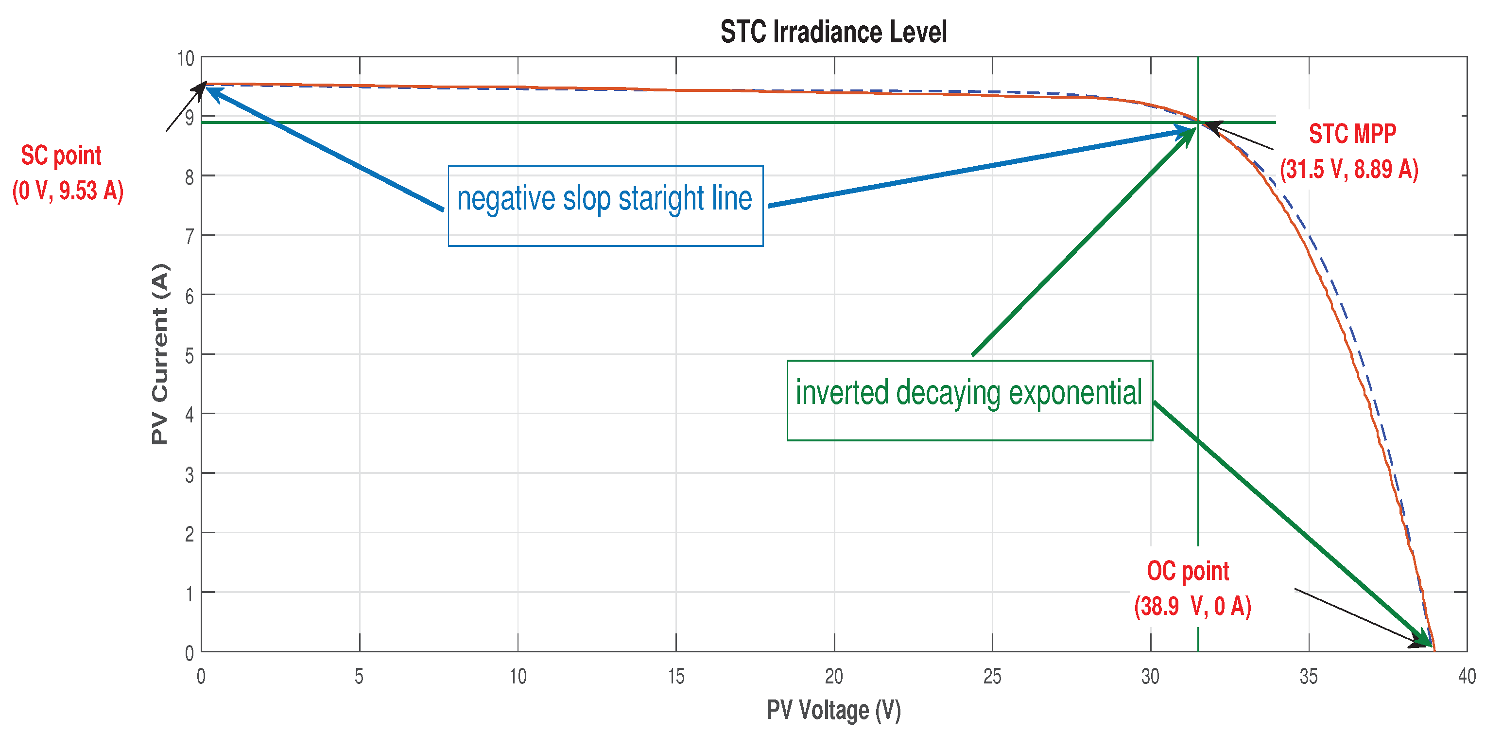
The proposed model is developed based on analyzing the I–V curves in several datasheets. By analyzing the curves we observed that the curve can be represented in the form of combination of two mathematical functions. The first function is negative slop straight line and the second one is inverted decaying exponential function. Varying the values of irradiance and temperature have nearly a scaling effect on the I–V curve shape but with preserving the same form. Therefore, the empirical mathematical model proposed in this paper is developed over two stages. The first one is to resemble the curve features in terms of the STC electrical performance terms. The second stage is to represent the impact of varying levels of irradiance and/or temperature on the curves to generalize the model.
In datasheets, it is common to include the curves of the varying irradiance at fixed temperature and/or varying temperature at fixed irradiance. Some datasheets also include a general case at a certain value of irradiance and temperatures which differ from the STC conditions. Therefore, the proposed model is considered over three cases: (i) varying the irradiance levels at STC temperature value, (ii) varying the temperature values at STC irradiance level, and (iii) general form at any value of irradiance and temperature. Each case of them is represented with separate model.
By investigating the first case of different irradiance level at the STC temperature value ( T 0 = 25 °C) the effect of this change on the current and voltage is presented for any value of irradiance relative to the STC one as a scale ratio. However, for the second case, the effect of changing the temperature values at the STC irradiance level ( G 0 = 1000 W/m2) is represented in the model with a different ratio of temperature change, producing another form of the model generating the curves at any temperature value at STC irradiance level.
Finally, the general case of producing the curve at any environmental condition different from the STC case is investigated and presented in a general form of the proposed empirical mathematical model after updating the electrical terms used over two passes, one for new irradiance level and STC temperature then for new condition of both new irradiance and temperature required conditions.
The following subsections demonstrate each case of the three models and the used electrical performance terms notations in the models are defined as the following:
G:Irradiance Level G 0 :STC Irradiance Level
T:Temperature Value T 0 :STC Temperature Value
I M P P :Maximum Power Current V M P P :Maximum Power Voltage
I S C :Short Circuit Current V O C :Open Circuit Voltage

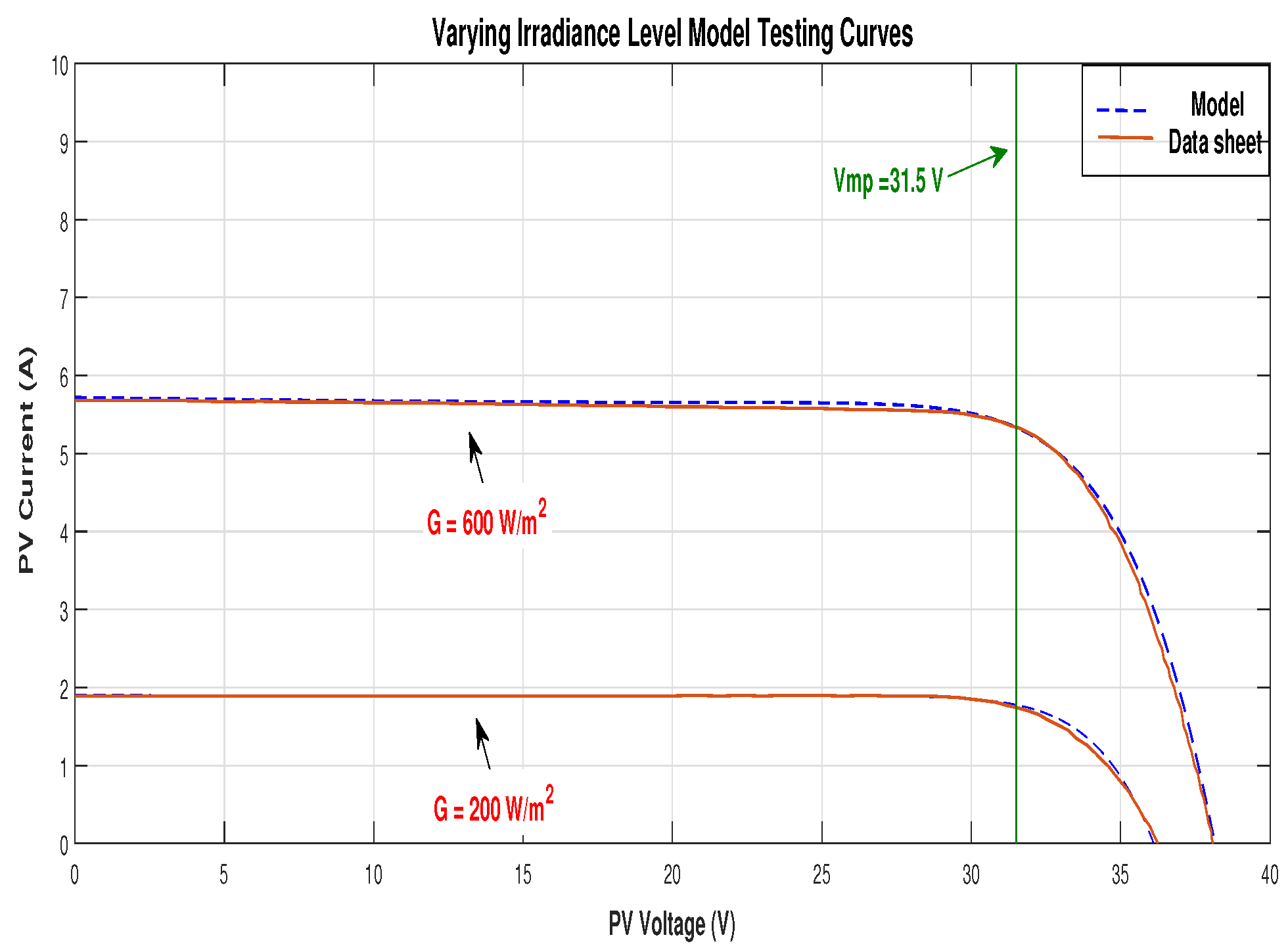
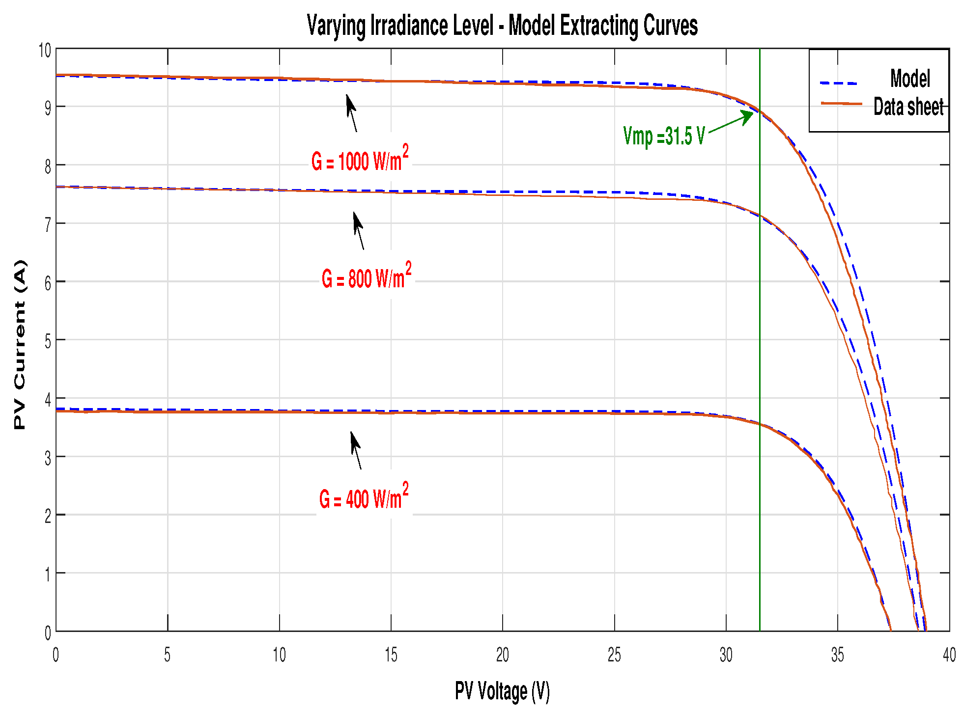
4.1. Case One: I–V Characteristics Empirical Mathematical Model for Varying Irradiance Levels

The varying irradiance level leads to varied values of the current produced by the PV panel with the same curve features mentioned early as a combination of two mathematical functions, (i) negative slop straight line and (ii) inverted decaying exponential function. Therefore, with decreasing the irradiance value the current decreases with a ratio of the irradiance level to STC level. In addition, the value of the open circuit voltage reduces with the exponential reduction in the irradiance amount. The maximum power point voltage value is independent of irradiance level, so it is constant for all its values.
The current for any irradiance value at STC temperature value can be calculated using the shown Equation (1):
I ( G , T 0 ) = R × C + M × V B × 1 e x p V V O C ( G , T 0 ) × 1 e x p A [ V V M P P ( G 0 , T 0 ) ]
where,
R = G G 0 V O C ( G , T 0 ) = V O C ( G 0 , T 0 ) ( 1 R ) × V M P P ( G 0 , T 0 ) I M P P ( G 0 , T 0 ) ( 1 R ) V O C ( G 0 , T 0 ) V M P P ( G 0 , T 0 ) C = I S C ( G 0 , T 0 ) M = I M P P ( G 0 , T 0 ) I S C ( G 0 , T 0 ) V M P P ( G 0 , T 0 ) B = e x p V M P P ( G 0 , T 0 ) V O C ( G , T 0 ) a = 1 + V O C ( G , T 0 ) V V M P P ( G 0 , T 0 ) 1 V O C ( G , T 0 ) V M P P ( G 0 , T 0 ) A = a × ln 1 ( C + M × V O C ( G , T 0 ) ) B ( 1 e )

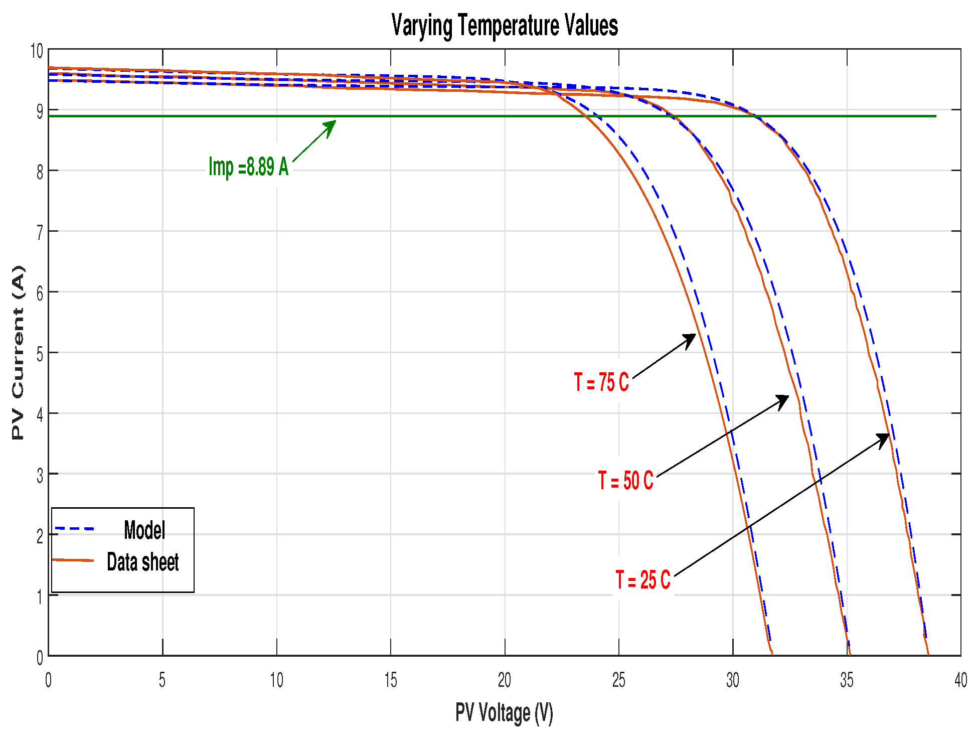
4.2. Case Two: I–V Characteristics Empirical Mathematical Model for Varying Temperature Levels

The same equation previously mentioned in Equation (1) is used to find the I–V curve at fixed level of irradiance (STC level), and any temperature values, but with updated values of some electrical performance terms. The change in temperature at fixed irradiance level has an effect on the values of the short circuit current, open circuit voltage, and maximum power point voltage, although the maximum power point current is constant for various temperature values.
The current for any temperature value at STC irradiance level can be calculated using the shown Equation (2):
I ( G 0 , T ) = C + M × V B × 1 e V V O C ( G 0 , T ) × 1 e A × ( V V M P P ( G 0 , T ) )
where,
S = T T 0 T 0 I S C ( G 0 , T ) = I S C ( G 0 , T 0 ) + 0.1 × S V O C ( G 0 , T ) = V O C ( G 0 , T 0 ) S × V M P P ( G 0 , T 0 ) 1 I M P P ( G 0 , T 0 ) V M P P ( G 0 , T ) = V M P P ( G 0 , T 0 ) e S I M P P ( G 0 , T 0 ) 2 V M P P ( G 0 , T 0 ) C = I S C ( G 0 , T ) M = I M P P ( G 0 , T 0 ) I S C ( G 0 , T ) V m p ( G 0 , T ) B = e V M P P ( G 0 , T ) V O C ( G 0 , T ) a = 1 + V O C ( G 0 , T ) V V M P P ( G 0 , T ) 1 V O C ( G 0 , T ) V M P P ( G 0 , T ) A = a × ln 1 ( C + M × V O C ( G 0 , T ) ) B ( 1 e )

4.3. Case Three: I–V Characteristics Empirical Mathematical Model for Certain Irradiance and Temperature Values

The current at STC irradiance and temperature values can be produced using either Equation (1) for the case where R = 1 a t G = G 0 or Equation (2) at the case of S = 0 a t T = T 0 . However, to generate a curve of PV-panel current output at a certain irradiance and temperature level different from the STC, the same equation is used after updating the model electrical performance terms over two phases, one for updating irradiance to new level, and one updating for the new temperature value, as illustrated below:
Phase one: calculate terms for required irradiance value and at STC temperature ( G , T 0 ) , the following equations are used to find the updated values:
R = G G 0 V O C ( G , T 0 ) = V O C ( G 0 , T 0 ) ( 1 R ) V M P P ( G 0 , T 0 ) I M P P ( G 0 , T 0 ) ( 1 R ) V O C ( G 0 , T 0 ) V M P P ( G 0 , T 0 ) I S C ( G , T 0 ) = R I S C ( G 0 , T 0 ) I M P P ( G , T 0 ) = R I M P P ( G 0 , T 0 ) V M P P ( G , T 0 ) = V M P P ( G 0 , T 0 )
Phase two: based on the values generated from phase one to find the terms for the required environmental condition ( G , T ) , the following equations are used, resulting in the updated values:
S = T T 0 T 0 V O C ( G , T ) = V O C ( G , T 0 ) S V M P P ( G 0 , T 0 ) 1 I M P P ( G 0 , T 0 ) I S C ( G , T ) = I S C ( G , T 0 ) + 0.1 S I M P P ( G , T ) = I S C ( G , T 0 ) V M P P ( G , T ) = V M P P ( G , T 0 ) e S I M P P ( G 0 , T 0 ) 2 V M P P ( G 0 , T 0 )
After updating the electrical terms for the required irradiance and temperature values the I–V curve is calculated using the following Equation (3):
I ( G , T ) = C + M × V B × 1 e V V O C ( G , T ) × 1 e A ( V V M P P ( G , T ) )
where,
C = I S C ( G , T ) M = I M P P ( G , T ) I S C ( G , T ) V M P P ( G , T ) B = e V M P P ( G , T ) V O C ( G , T ) a = 1 + V O C ( G , T ) V V M P P ( G , T ) 1 V O C ( G , T ) V M P P ( G , T ) A = a × ln 1 ( C + M × V O C ( G , T ) ) B ( 1 e )

5. Proposed Model Simulation

The datasheet of the PV-panel KYOCERA PV-model (KK280P-3CD3CG) [63] is to develop and test the model. Developing the empirical model, at least three curves are needed, including the STC one which the model is based on, scaling it with varying the irradiance or the temperature values. The remaining unused curves are used to test the model. The extracted data versus the curves produced from the proposed mathematical empirical model is presented in the following subsection as follows:
  • STC case curve.
  • Varying irradiance levels at fixed STC temperature.
  • Testing the proposed model with the unused irradiance levels at fixed STC temperature.
  • Varying temperature values at fixed STC irradiance.
The standard electrical performance testing condition values used in simulating the curves are listed below in Table 1:

5.1. Simulation of I–V Characteristics Curves Generated by the Mathematical Model

The STC case (G = 1000 W/m2 and T0 = 25 °C) is simulated using the proposed mathematical model and the produced I–V curve is compared with the data extracted from the datasheet [63], as shown in the following Figure 15.

5.2. Simulation of I–V Characteristics Curves for Varying Irradiance Levels at Fixed STC Temperature

Three curves at different levels of irradiance are used to develop the model including the STC one at fixed STC temperature value. The model is simulated for the irradiance levels (G = 400, 800, and 1000 W/m2) at fixed temperature value of STC case T0 = 25 °C and both the mathematical model and the datasheet current values are presented in Figure 16.
As shown in the results, with the irradiance value decreasing, the current decreases as well. Additionally, the value of the open circuit voltage reduces with a reduction in the irradiance amount on the cell. The maximum power point voltage value is fixed for all irradiance levels.

5.3. Testing the Proposed Model with the Unused Irradiance Levels at Fixed STC Temperature

The model is tested using the rest of the irradiance levels (200, 600 W/m2) at fixed temperature value of STC case T0 = 25 °C, and both the mathematical model and the datasheet current values are presented in Figure 17.
As shown from the simulation, the model is performing reasonably compared to the actual extracted data.

5.4. Simulation of I–V Characteristics Curves for Varying Temperature Values at Fixed STC Irradiance Level

The model is simulated with varying the values of temperature from 25 °C to 75 °C at fixed irradiance level of STC case G 0 = 1000 W/m2 and both the mathematical proposed model and the datasheet current values are shown in Figure 18.
The results of varying temperatures show that, with increasing temperature, the maximum power point voltage and the value of the open circuit voltage decreases. The maximum power point current value is fixed for different values of temperatures.

6. Model Validation

In this section, various datasheets with different ranges of output power ratings are used to validate the proposed empirical mathematical model. The electrical performance values of STCs of each PV-panel with its rating power are shown in Table 2. Figure 19, Figure 20, Figure 21 and Figure 22 present the I–V curves of the used datasheet for validating the proposed empirical mathematical model for different irradiance and temperature levels.
To add to the proposed model validation, the root mean square error (RMSE) between the PV I–V curves, modeled by the proposed approach, and their relative experimental datasheet curves are computed and presented in the tables below. The following Table 3 and Table 4 present the root mean square error calculated for various irradiance levels and temperature values, respectively. It is noted that, for the tested PV models, the RMSE under different irradiance levels is less than 0.4 in most severe cases (at 1000 W/m2) which verifies the proposed approach capability during different irradiances. During varying temperatures, the proposed approach shows high performance encountering RMSE less than 0.4 for temperatures ≥25 °C. However, at severe temperature cases (temperatures ≤10 °C), RMSE reaches high levels which show the proposed model limitations at very low temperatures.

7. Comparison of the Proposed Model with a Single Diode Equivalent-Circuit Based Model

In this section, a comparison between the proposed empirical mathematical PV model and conventional model is presented in order to verify the proposed model. The conventional model is an equivalent circuit-based iterative approach and it is derived for single diode equivalent circuit with the I–V equation given by Equation (4):
I = I P V I 0 [ e x p V + R s I V t a 1 ] V + R s I R P
where, V t which is equal to N s K T q , is the PV thermal voltage with N s PV cells connected in series, q is the electron charge ( 1.60217646 × 10 19 C), K is the Boltzmann constant ( 1.3806503 × 10 23 J/°K), T (in °K) is the temperature of the pn junction.
Unlike the proposed approach, which only requires four electrical terms ( V O C ,   I S C , V M P P , and I M P P ) obtained from PV datasheet, the iterative model requires seven electrical terms ( V O C , I S C , V M P P , I M P P , K v ,   K I , and N s ) as well as an iterative parameters extraction procedure. The latter puts a random estimation for the ideality factor ( a ) , uses an analytical equation to compute I o , and finally applies a numerical iterative method to compute R s then R p and I p v . The curves fitting steps can be summarized as follows [7];
  • a is selected in the range 1 a 1.5 . In the considered case, a is chosen to be 1.25 .
  • I 0 is computed using Equation (5)
    I 0 = I S C + K I Δ T e x p V O C + K V Δ T V t a 1
    Δ T = T T 0 (T and T 0 are the actual and STC temperatures, respectively, (in °K)).
  • R s and R P are calculated using an iterative method shown in Figure 23.
    -
    R s is slowly incremented starting from R s = 0
    -
    R P = R P m i n = V M P P I S C I M P P V O C V M P P I M P P
    -
    Several values of R s and R p are calculated till the P–V curve peak power P M P P coincides with the experimental peak power P M P P e given by datasheet (=135 W in the considered case).
    -
    The relation between R s and R p , can be found by making P M P P = P M P P e and solving the resulting equation to find R P as shown in Equations (6) and (7)
    P M P P = V M P P I p v I 0 e x p q K T V M P P + R s I M P P N s a 1 V M P P + R s I M P P R P
    R P = V M P P ( V M P P + R s I M P P ) V M P P I p v V M P P I 0 e x p q K T V M P P + R s I M P P N s a + V M P P I 0 P M P P e
    In the considered case, the resistances are found to be R s = 0.18 Ω and R p = 63 Ω for a peak power tolerance of 0.1 W.
  • Calculate the light-generated current at the considered conditions ( I p v ) from the nominal light-generated current ( I p v n ) using Equation (8)
    I p v = ( I p v n + K I Δ T ) G G 0
    where, I p v n = R P + R s R P I S C and (W/m2) is the irradiation on the device surface, and G 0 is the STC irradiation.
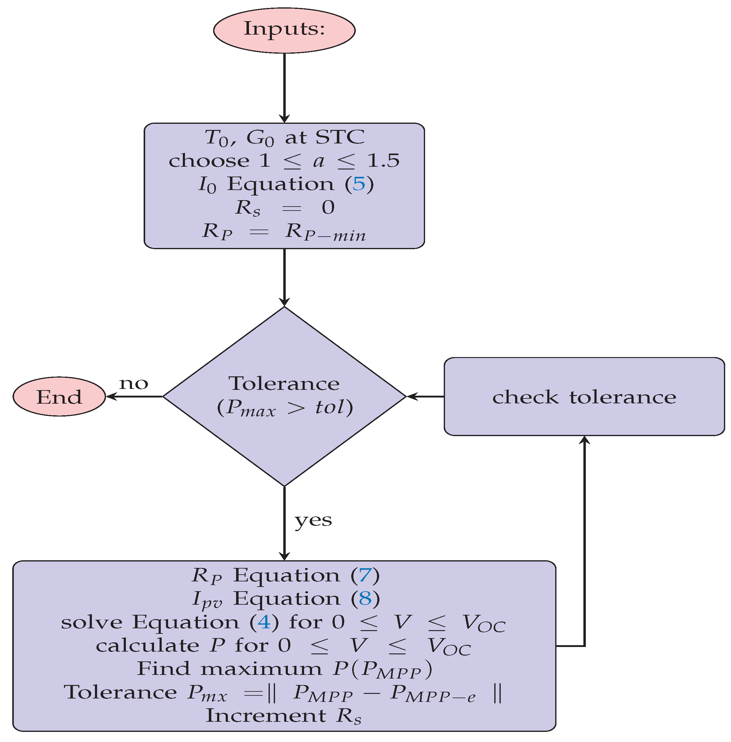
The iterative method flowchart applied for finding R s and R p is shown in Figure 23. Both models are validated using the ratings of K D 135 S X - U P U [68] module PV with datasheet parameters shown in Table 5.
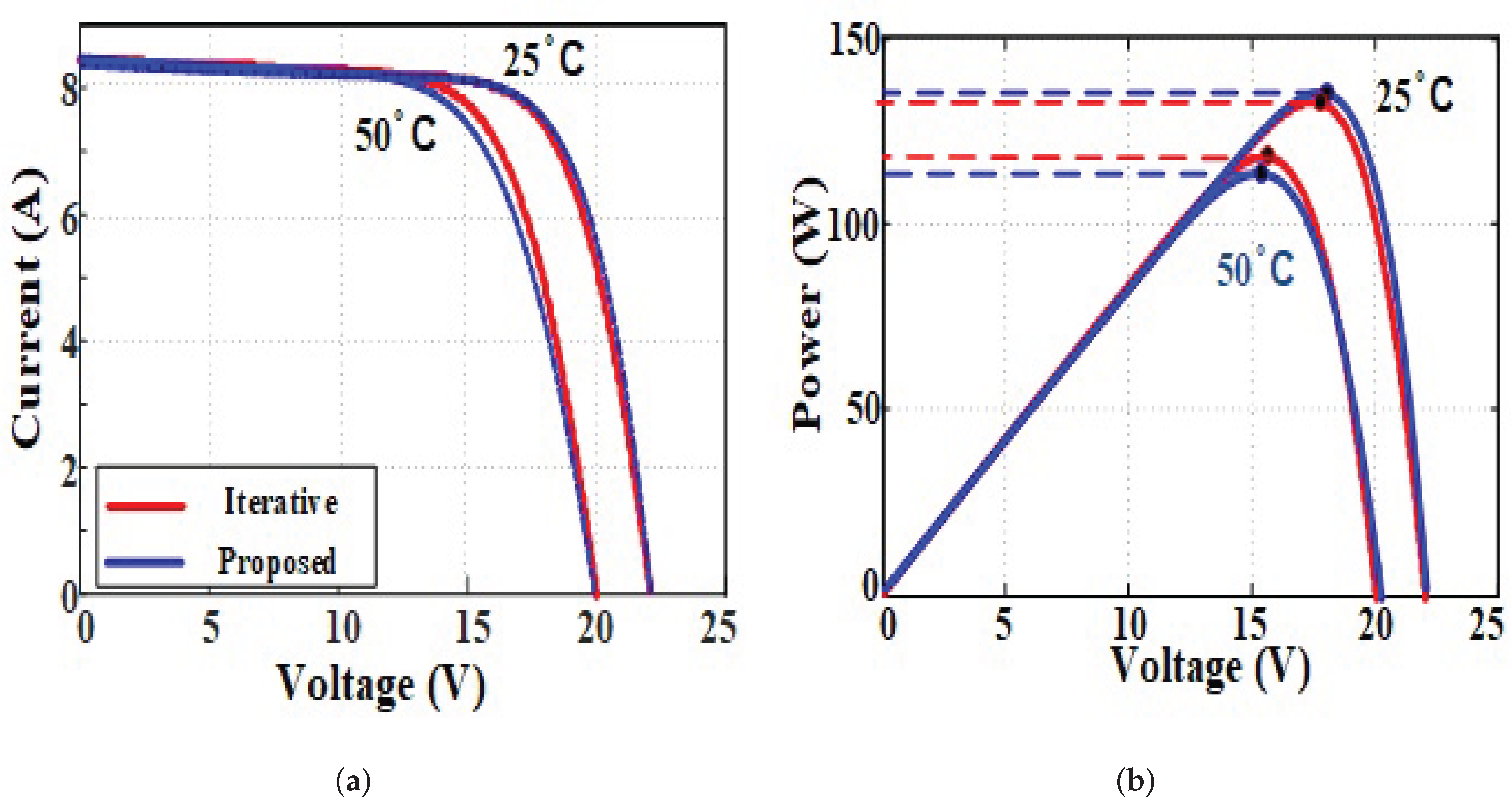
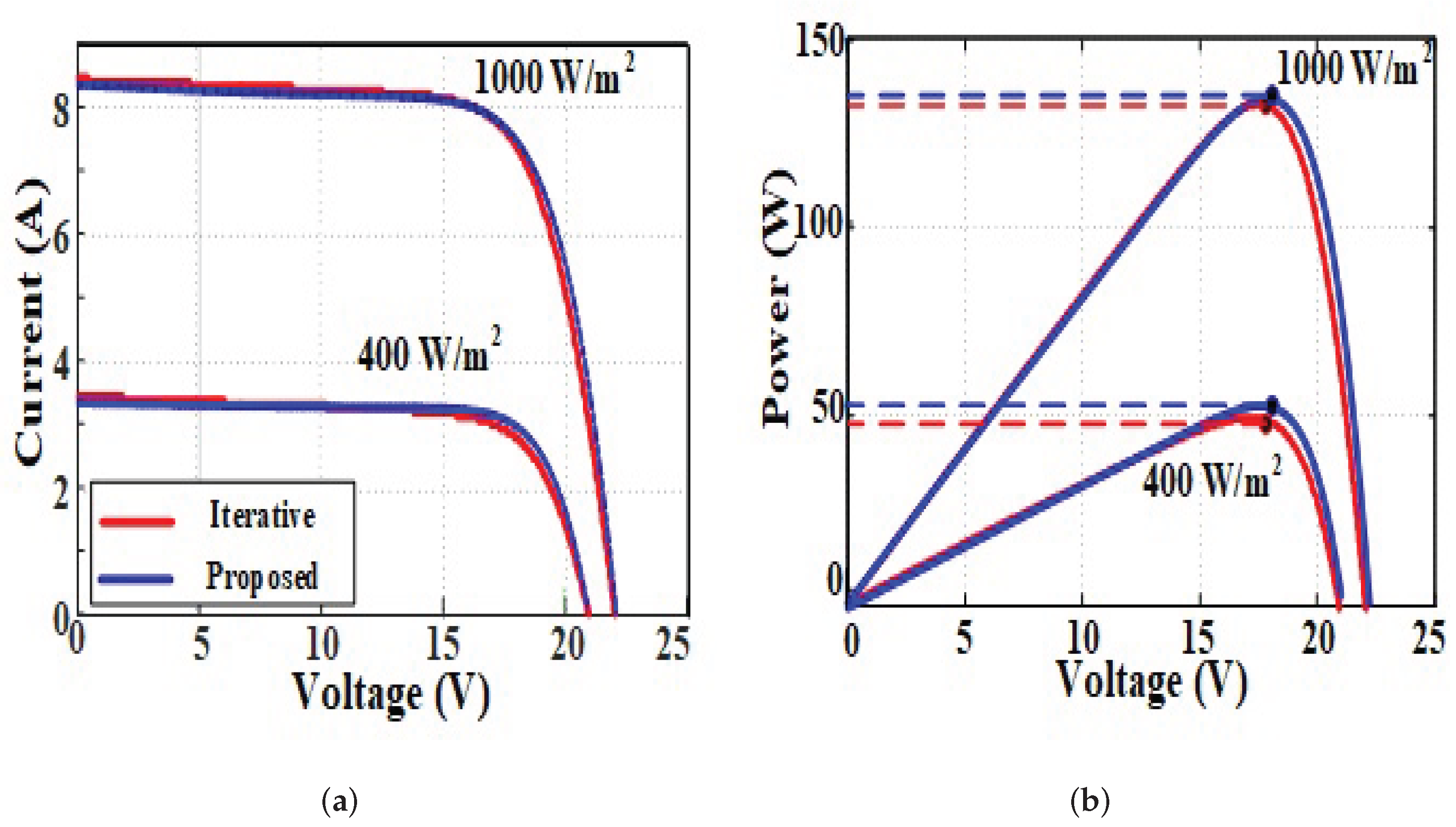
The simulation comparison results of the two models are shown in Figure 24 that represents the performance for different irradiance levels and Figure 25 which represents the performance for different temperature values. Each figure include both I–V and P–V curves to illustrate the variance in the performance of the two models. From the simulation results of the conventional model and the proposed mathematical model it was found that the performance of the proposed one deliver better accuracy as its maximum power value is 135.056 W where the conventional model maximum power is 134.15 W for the same datasheet ratings at STC condition. This verifies the proposed model’s effectiveness, yet with simpler implementation and less computational time and efforts when compared to the iterative model. The proposed model depends solely on a generic empirical equation that requires only four basic electrical terms found in any PV datasheet without the need for any parameter estimation.
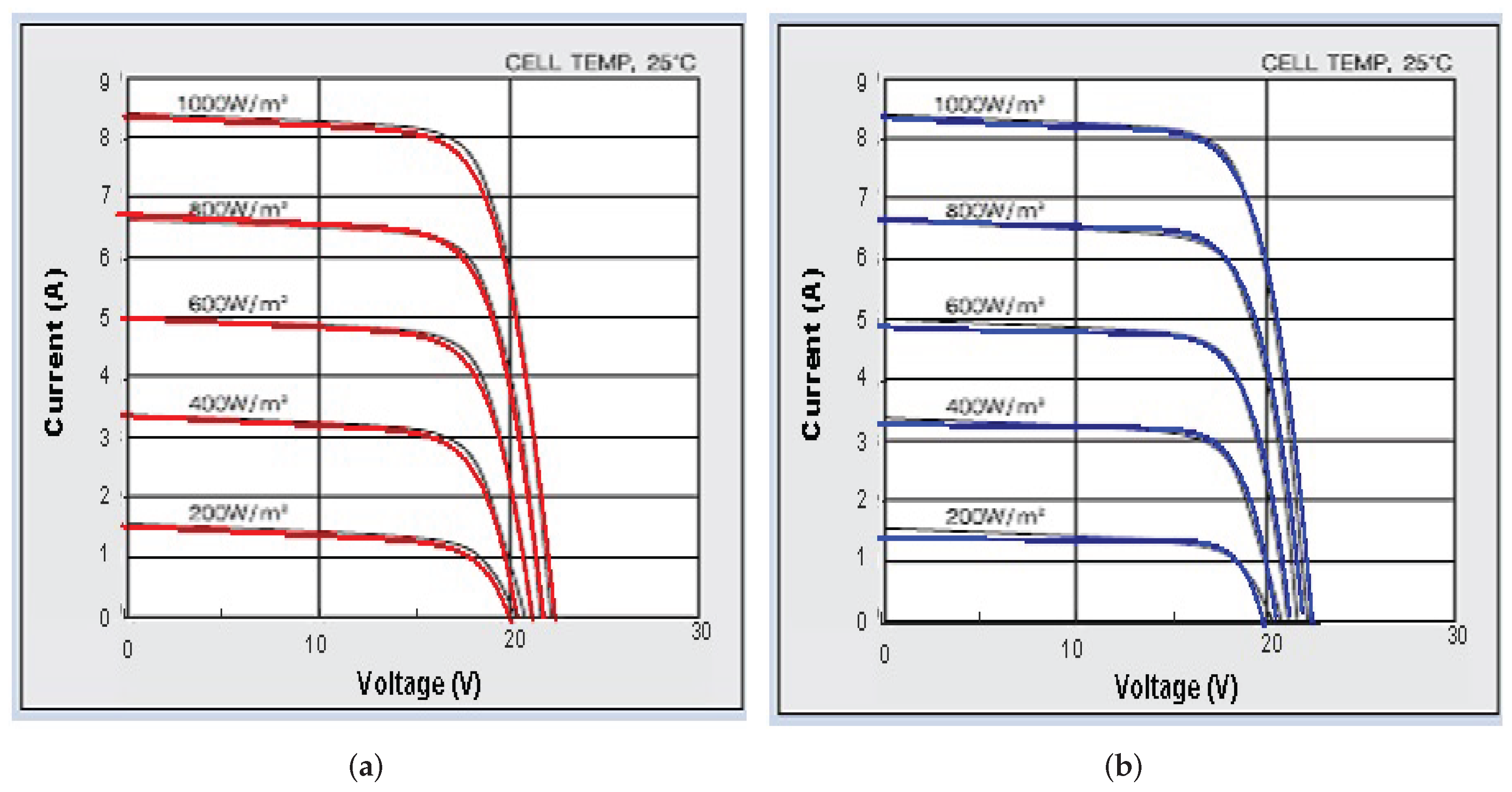
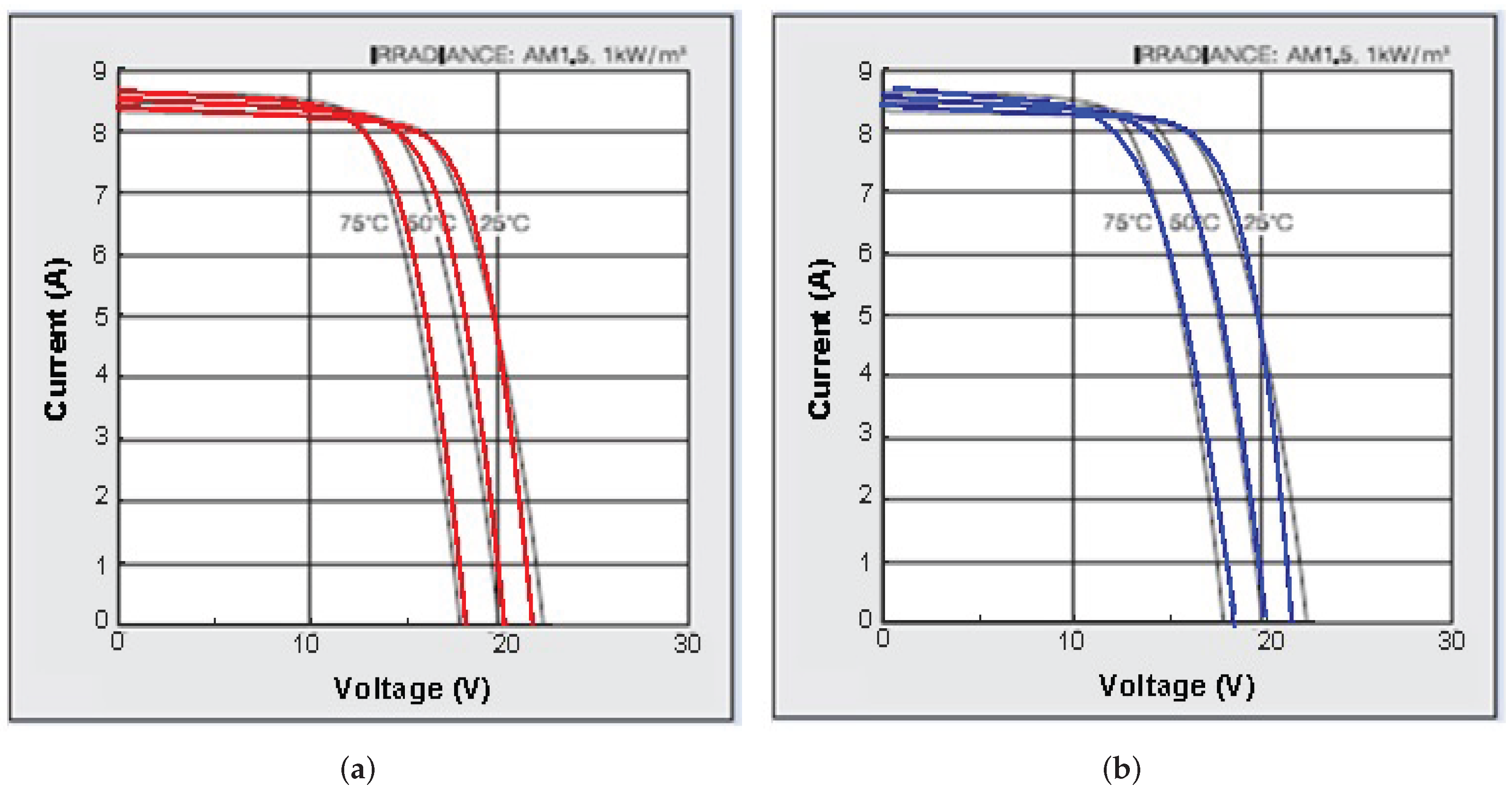
The proposed approach-based I–V curves versus the iterative approach-based ones, for K D 135 S X - U P U PV module, are compared to those of the P–V experimental datasheet curves. As shown in Figure 26 and Figure 27, these comparisons are achieved at all the irradiance and temperature levels presented by the experimental datasheet curves which include low irradiance cases. Results show that both approaches gave close I–V curves to those experimental ones presented in datasheet. However, this is achieved with the proposed simpler, faster, less parameter-dependent, and iteration-free empirical method.
For further validation, the latter is retested with a different PV panel with different rating from another manufacturer, the K C 200 G T PV-module, with specifications presented in Table 6. The experimental I–V curves applied are shown in Figure 28 and Figure 29. Results confirm that both techniques experience relatively close I–V curves which fit onto the experimental curves of this module with the datasheet given below:

8. Privileges and Limitations Discussion

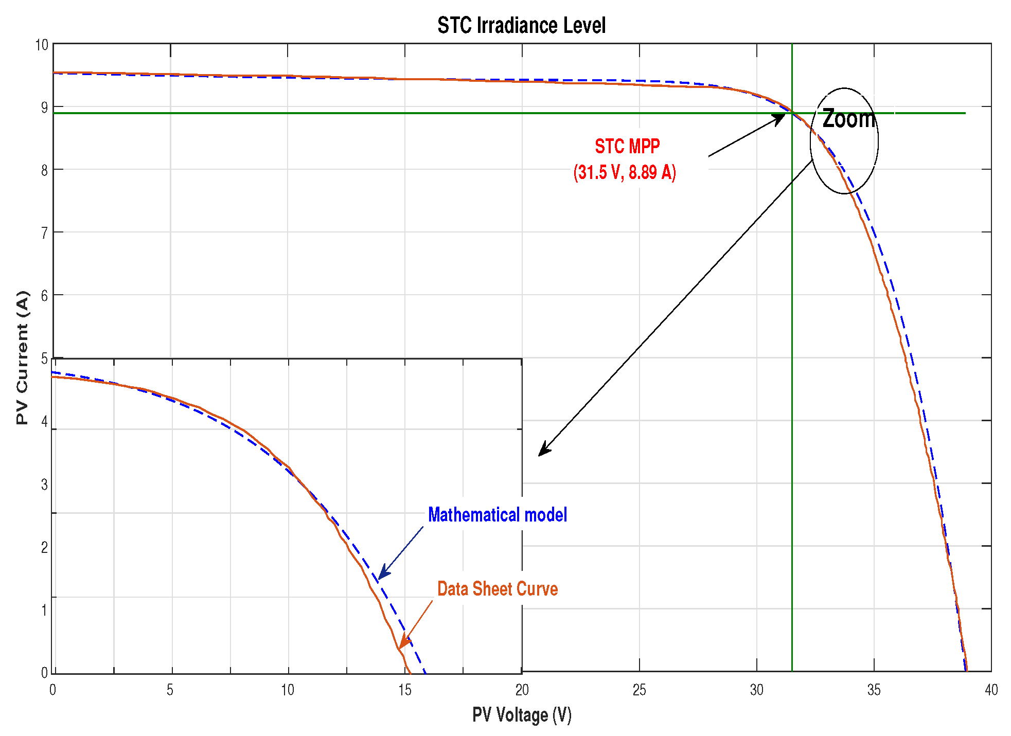
The proposed empirical method is based mainly on the mathematical representation of experimental I–V curves extracted from a PV module datasheet. The model formulates the STC case in mathematical function depending on only four electrical components of the PV-panel ( V O C ,   I S C , V M P P ,   I M P P ). By investigating the STC case I–V curve, it was found that the point of maximum power is a critical point that divides the curve into two parts. The one on the left, starting from the short circuit point and ending at the maximum power point, is a straight line with a negative slope. The equation of this line is formulated based on these two points of the start and end, so it is represented in terms of the electrical terms mentioned earlier. The other curve to the right of the maximum power point is behaving similarly to the inverted decaying exponential function. The two points used to formulate the power of this exponential function are the point of maximum power and the open circuit point. The PV-model proposed in the paper is based on combining these two functions together, that is, the basic equation which is used to generate the STC case curve, as shown in Figure 30. To represent the effect of changing in irradiance or temperature, the authors used other curves and investigated the impact of these changes on the curve relative to the STC case values.
It is worth nothing that this curve extraction is a one-time process, followed by the derivation of empirical equations that mathematically represent this curve for different irradiance and temperature conditions. These equations are valid for any other PV-model and can be applied for all PV ratings from different manufacturers i.e., any PV-module I–V characteristics and curves can be obtained by direct substitution of the new relative ( V O C ,   I S C , V M P P , and I M P P ) in the derived empirical equations. Unlike the proposed approach, the physical models depend more on electrical terms, and not all of them are available on datasheets. Thus, they require parameter extraction techniques which depend on iterative and estimation approaches, which in turn adds to system complexity and computational time.
The Table 7 summarizes the main differences between single-diode equivalent circuit-based iterative physical approach presented in Section 7 and the proposed empirical approach regarding approach realization, error cause, implementation complexity, and computational time.
The proposed model relies on data extracted from PV panel manufacturer datasheets available on the market. Commonly, those curves listed in various vendors are experimentally obtained to achieve proper standardized certification as IEC, IEEE, NEC, or UL. In addition, data extraction is only performed once, as stated and performed by the authors. Any further investigation of other PV panels from any other vendors do not require curve extraction, as explained. Only four parameters are needed to substitute in the authors’ pre-elaborated proposed formula. Hence, fear form any further unavailability of experimental datasheets is not crucial.
The proposed technique in this paper is developed by using the captured images from the datasheet only once, and then, for generating any graphs at various rating power, the developed proposed model is used directly. There is no need to capture the images from the datasheet every time for reproduction, as this model features the graphs in terms of the electric parameters of the PV-panel ( V O C ,   I S C , V M P P , and I M P P ). The developing process of the model used some curves from the main datasheet, then the rest of the curves were used for testing the model. After that, many datasheets at different rating power were used to validate the model. The authors generated the curves using the proposed model and compared them to the datasheet curves so these curves were not used to develop a newer model. The proposed model is formulated for generating I–V curves for three cases: (i) various irradiance level at fixed STC temperature (Equation (1)), (ii) various temperature levels at fixed irradiance level (Equation (2)), and (iii) certain value or irradiance and temperature differ from the STC case (Equation (3)).
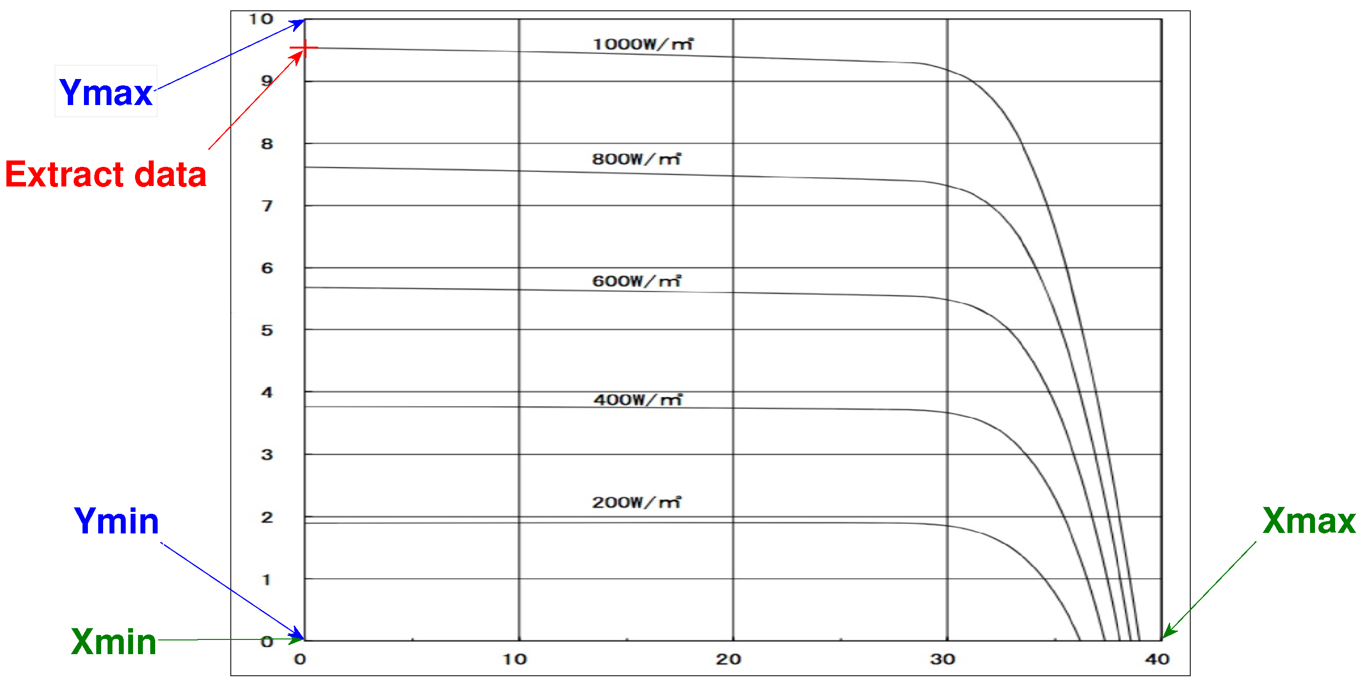
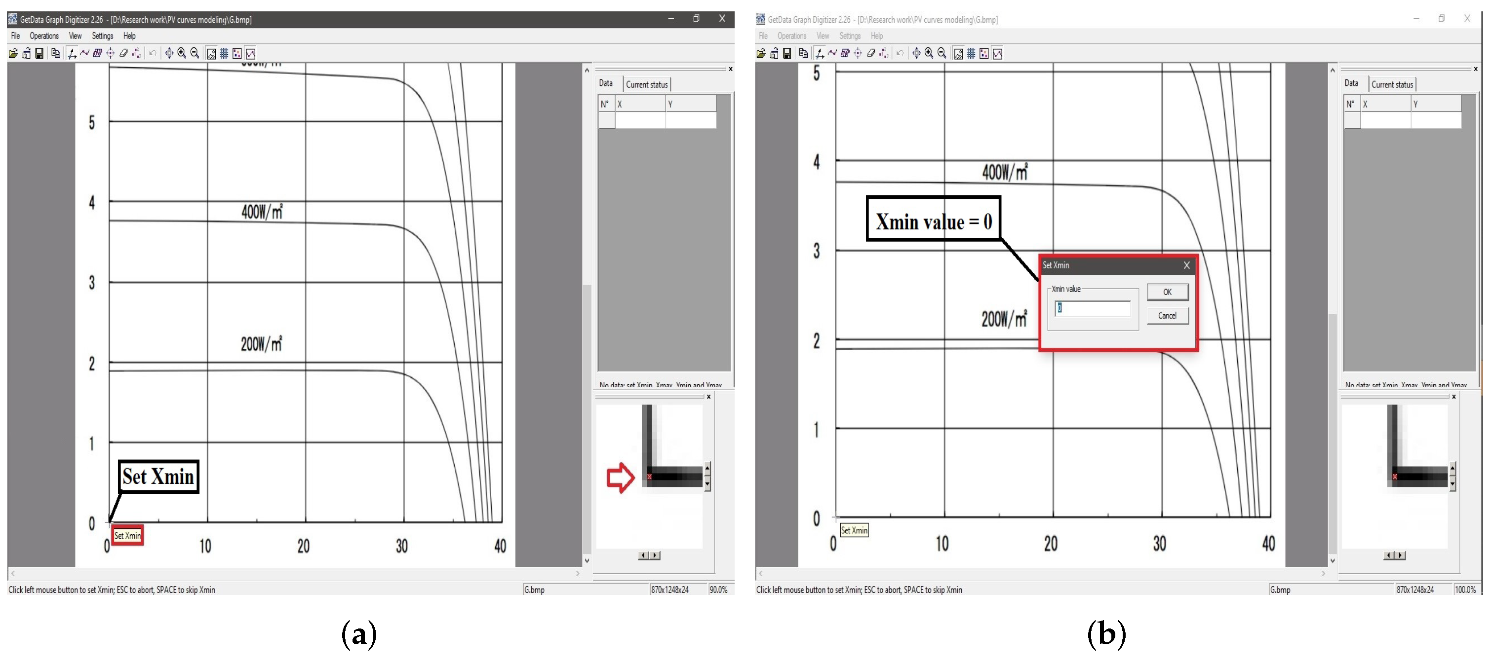
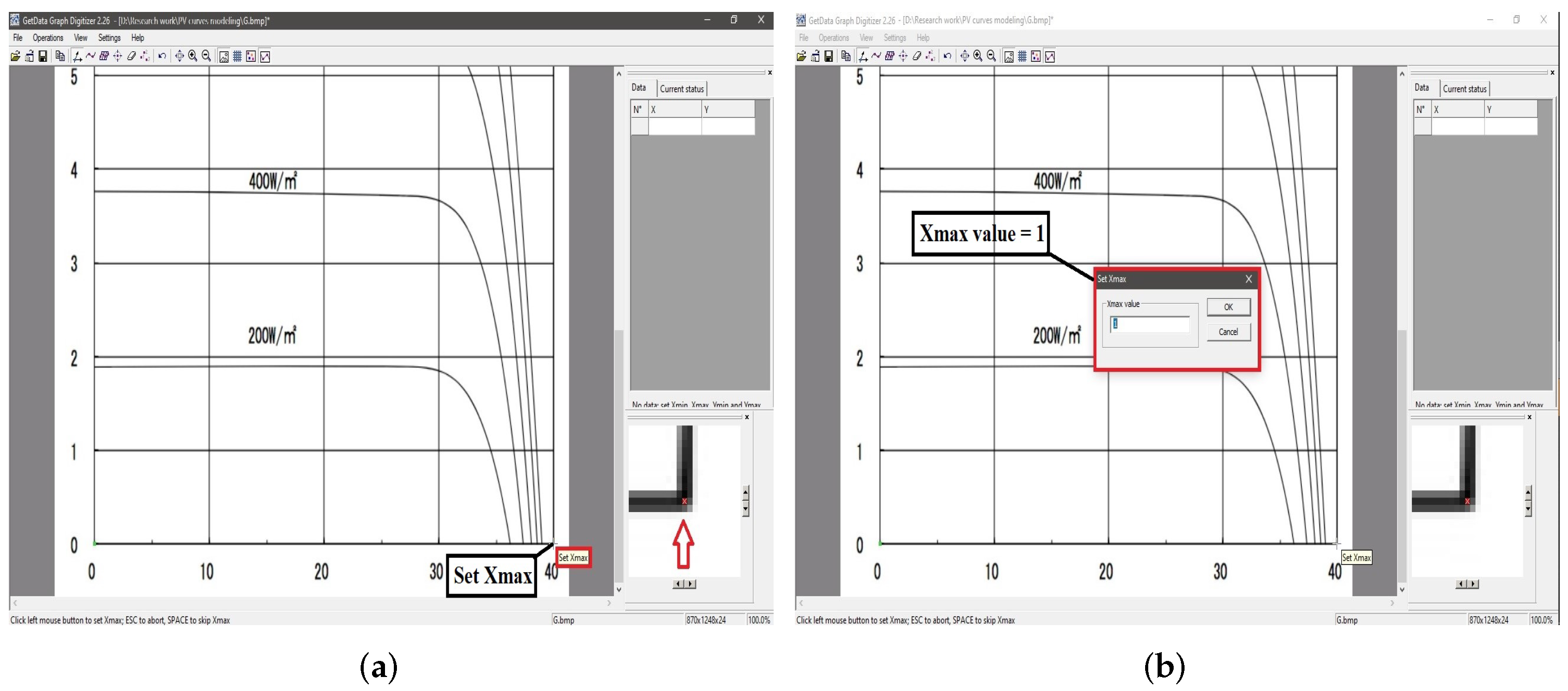
As the developed model is based on digitizing the characteristic curves captured from the datasheet there are some sources of error that affect the data accuracy. The first source of error is the resolution of the captured image from the datasheet. To overcome this source of error, aiming to enhance the accuracy of the extracted data from the datasheet, the authors used image editing software to increase the DPI of the figures.
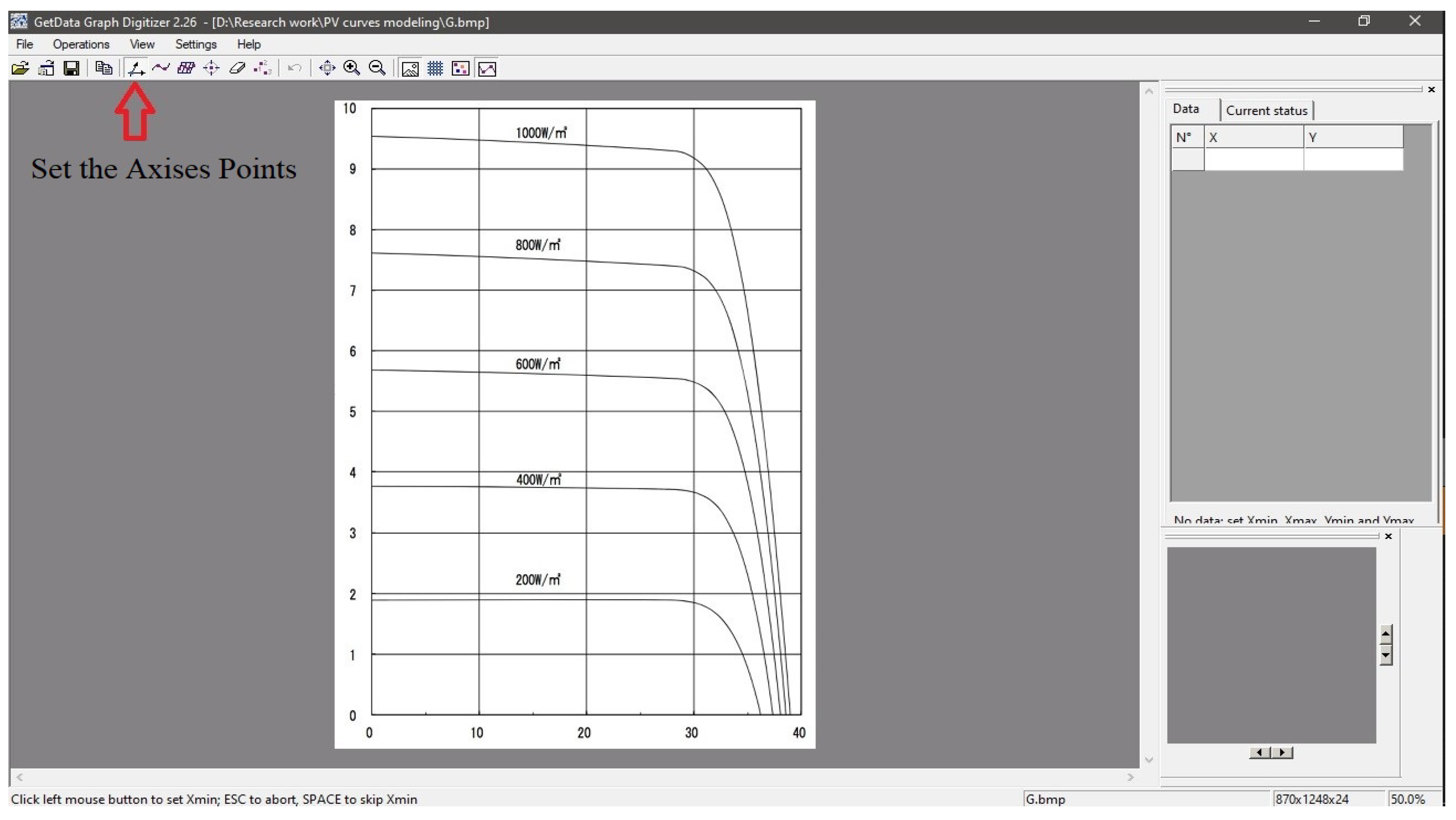
The second source of error is the manual selection of the graph points in order to extract its numerical value. To mitigate this source of error, the authors used many graph digitizing software packages and compared their output to select the software that delivers the most accurate data extraction. The manual process itself is, unfortunately, unavoidable.

9. Conclusions

In this paper, a novel generic empirical mathematical formula is proposed to model any PV device at varying conditions, based on function representation of captured PV experimental figures. This approach shows simpler implementation and less computational time and efforts when compared to existing PV models that require parameter estimation or power forecast. However, this apporach also offers competitive accuracy. PV curves resulting from the proposed formula show close resemblance to experimental curves of practical PV devices at different environmental conditions. The proposed formula’s effectiveness is verified using commercial, market-available PV panels from different manufacturers at various power ratings to highlight the claimed robust performance and accurate PV device modeling features. The proposed PV model can be implemented on a graphical user interface GUI toolbox, presented as a user-friendly block for energy system designers and circuit simulator developers. This facilitates the simulation of PV devices their performance during dynamic shading and address the MPPT problem to assess.

Author Contributions

Conceptualization, A.A.; Data curation, O.H. and N.Z.; Formal analysis, O.H. and A.A.; Investigation, O.H. and A.A.; Methodology, N.Z. and A.A.; Software, O.H.; Supervision, A.A.; Validation, O.H. and N.Z.; Visualization, O.H.; Writing—original draft, O.H. and N.Z.; Writing—review & editing, A.A. All authors have read and agreed to the published version of the manuscript.

Funding

This research received no external funding.

Data Availability Statement

Not applicable.

Conflicts of Interest

The authors declare no conflict of interest.

References

  1. SunShot Vision Study- Photovoltaics: Technologies, Cost, and Performance; U.S. Department of Energy: Washington, DC, USA, 2012.
  2. Hosenuzzaman, M.; Rahim, N.; Selvaraj, J.; Hasanuzzaman, M.; Malek, A.; Nahar, A. Global prospects, progress, policies, and environmental impact of solar photovoltaic power generation. Renew. Sustain. Energy Rev. 2015, 41, 284–297. [Google Scholar] [CrossRef]
  3. Eltamaly, A.M.; Farh, H.M.H. PV Characteristics, Performance and Modelling. In Modern Maximum Power Point Tracking Techniques for Photovoltaic Energy Systems; Eltamaly, A.M., Abdelaziz, A.Y., Eds.; Springer International Publishing: Cham, Switzerland, 2020; pp. 31–63. [Google Scholar]
  4. Onat, N. Recent Developments in Maximum Power Point Tracking Technologies for Photovoltaic Systems. Int. J. Photoenergy 2010, 2010, 245316. [Google Scholar] [CrossRef] [Green Version]
  5. Jakhrani, A.Q.; Othman, A.K.; Rigit, A.R.H.; Samo, S.R. Model for estimation of global solar radiation in Sarawak, Malaysia. World Appl. Sci. J. 2011, 14, 83–90. [Google Scholar]
  6. Ramaprabha, R.; Mathur, B.L. Development of an improved model of SPV cell for partially shaded solar photovoltaic arrays. Eur. J. Sci. Res. 2010, 47, 122–134. [Google Scholar]
  7. Villalva, M.; Gazoli, J.; Filho, E. Comprehensive approach to modeling and Simulation of Photo-voltaic Arrays. IEEE Trans. Power Electron. 2009, 24, 1198–1208. [Google Scholar] [CrossRef]
  8. Xiao, W.; Dunford, W.; Capel, A. A novel modeling method for photovoltaic cells. In Proceedings of the 2004 IEEE 35th Annual Power Electronics Specialists Conference (IEEE Cat. No.04CH37551), Aachen, Germany, 20–25 June 2004; Volume 3, pp. 1950–1956. [Google Scholar]
  9. Guidelines for PV Power Measurement in Industry; European Commission Joint Research Centre (JRC), Institute of Energy: Ispra, Italy, 2010.
  10. Soto, W.D.; Klein, S.A.; Beckman, W.A. Improvement and validation of a model for photovoltaic array performance. Sol. Energy 2006, 80, 78–88. [Google Scholar] [CrossRef]
  11. Carrero, C.; Amador, J.; Arnaltes, S. A single procedure for helping PV designers to select silicon PV modules and evaluate the loss resistances. Renew. Energy 2007, 32, 2579–2589. [Google Scholar] [CrossRef]
  12. Veerachary, M. PSIM circuit-oriented simulator model for the nonlinear photovoltaic sources. IEEE Trans. Aerosp. Electron. Syst. 2006, 42, 735–740. [Google Scholar] [CrossRef]
  13. Kim, W.; Choi, W. A novel parameter extraction method for the one diode solar cell model. Sol. Energy 2010, 84, 1008–1019. [Google Scholar] [CrossRef]
  14. Xiao, W.; Edwin, F.F.; Spagnuolo, G.; Jatskevich, J. Efficient Approaches for Modeling and Simulating Photovoltaic Power Systems. IEEE J. Photovoltaics 2013, 3, 500–508. [Google Scholar] [CrossRef]
  15. Breitenstein, O. An Alternative One-Diode Model for Illuminated Solar Cells. IEEE J. Photovoltaics 2014, 4, 899–905. [Google Scholar] [CrossRef]
  16. Sandrolini, L.; Artioli, M.; Reggiani, U. Numerical method for the extraction of photovoltaic module double-diode model parameters through cluster analysis. Appl. Energy 2010, 87, 442–451. [Google Scholar] [CrossRef]
  17. Ishaque, K.; Salam, Z.; Taheri, H. Simple, fast and accurate two-diode model for photovoltaic modules. Sol. Energy Mater. Sol. Cells 2011, 95, 586–594. [Google Scholar] [CrossRef]
  18. Romero, B.; Pozo, G.; Arredondo, B. Exact analytical solution of a two diode circuit model for organic solar cells showing S-shape using Lambert Wfunctions. Sol. Energy 2012, 86, 3026–3029. [Google Scholar] [CrossRef]
  19. Babu, B.C.; Gurjar, S. A Novel Simplified Two-Diode Model of Photovoltaic (PV) Module. IEEE J. Photovoltaics 2014, 4, 1156–1161. [Google Scholar] [CrossRef]
  20. Nishioka, K.; Sakitani, N.; Uraoka, Y.; Fuyuki, T. Analysis of multicrystalline silicon solar cells by modified 3-diode equivalent circuit model taking leakage current through periphery into consideration. Sol. Energy Mater. Sol. Cells 2007, 91, 1222–1227. [Google Scholar] [CrossRef]
  21. Soliman, M.A.; Hasanien, H.M.; Alkuhayli, A. Marine Predators Algorithm for Parameters Identification of Triple-Diode Photovoltaic Models. IEEE Access 2020, 8, 155832–155842. [Google Scholar] [CrossRef]
  22. Manuel Godinho Rodrigues, E.; Godina, R.; Marzband, M.; Pouresmaeil, E. Simulation and Comparison of Mathematical Models of PV Cells with Growing Levels of Complexity. Energies 2018, 11, 2902. [Google Scholar] [CrossRef] [Green Version]
  23. Bader, S.; Ma, X.; Oelmann, B. A Comparison of One- and Two-Diode Model Parameters at Indoor Illumination Levels. IEEE Access 2020, 8, 172057–172064. [Google Scholar] [CrossRef]
  24. Cotfas, D.; Cotfas, P.; Kaplanis, S. Methods to determine the dc parameters of solar cells: A critical review. Renew. Sustain. Energy Rev. 2013, 28, 588–596. [Google Scholar] [CrossRef]
  25. Chin, V.J.; Salam, Z.; Ishaque, K. Cell modelling and model parameters estimation techniques for photovoltaic simulator application: A review. Appl. Energy 2015, 154, 500–519. [Google Scholar] [CrossRef]
  26. Jordehi, A.R. Parameter estimation of solar photovoltaic (PV) cells: A review. Renew. Sustain. Energy Rev. 2016, 61, 354–371. [Google Scholar] [CrossRef]
  27. Hasan, M.; Parida, S. An overview of solar photovoltaic panel modeling based on analytical and experimental viewpoint. Renew. Sustain. Energy Rev. 2016, 60, 75–83. [Google Scholar] [CrossRef]
  28. Ibrahim, H.; Anani, N. Evaluation of Analytical Methods for Parameter Extraction of PV modules. Energy Procedia 2017, 134, 69–78. [Google Scholar] [CrossRef]
  29. Celik, A.N.; Acikgoz, N. Modelling and experimental verification of the operating current of mono-crystalline photovoltaic modules using four- and five-parameter models. Appl. Energy 2007, 84, 1–15. [Google Scholar] [CrossRef]
  30. Altas, I.H.; Sharaf, A. A Photovoltaic Array Simulation Model for Matlab-Simulink GUI Environment. In Proceedings of the 2007 International Conference on Clean Electrical Power, Capri, Italy, 21–23 May 2007; pp. 341–345. [Google Scholar]
  31. Ding, K.; Bian, X.; Liu, H.; Peng, T. A MATLAB-Simulink-Based PV Module Model and Its Application Under Conditions of Nonuniform Irradiance. IEEE Trans. Energy Convers. 2012, 27, 864–872. [Google Scholar] [CrossRef]
  32. Aldwane, B. Modeling, simulation and parameters estimation for Photovoltaic module. In Proceedings of the 2014 First International Conference on Green Energy ICGE 2014, Sfax, Tunisia, 25–27 March 2014; pp. 101–106. [Google Scholar]
  33. Tan, Y.T.; Kirschen, D.; Jenkins, N. A model of PV generation suitable for stability analysis. IEEE Trans. Energy Convers. 2004, 19, 748–755. [Google Scholar] [CrossRef]
  34. Benavides, N.D.; Chapman, P.L. Modeling the effect of voltage ripple on the power output of photovoltaic modules. IEEE Trans. Ind. Electron. 2008, 55, 2638–2643. [Google Scholar] [CrossRef]
  35. Saloux, E.; Teyssedou, A.; Sorin, M. Explicit model of photovoltaic panels to determine voltages and currents at the maximum power point. Sol. Energy 2011, 85, 713–722. [Google Scholar] [CrossRef]
  36. Jain, A.; Kapoor, A. Exact analytical solutions of the parameters of real solar cells using Lambert W-function. Sol. Energy Mater. Sol. Cells 2004, 81, 269–277. [Google Scholar] [CrossRef]
  37. Jain, A.; Kapoor, A. A new method to determine the diode ideality factor of real solar cell using Lambert W-function. Sol. Energy Mater. Sol. Cells 2005, 85, 391–396. [Google Scholar] [CrossRef]
  38. Picault, D.; Raison, B.; Bacha, S.; de la Casa, J.; Aguilera, J. Forecasting photovoltaic array power production subject to mismatch losses. Sol. Energy 2010, 84, 1301–1309. [Google Scholar] [CrossRef]
  39. Chen, Y.; Wang, X.; Li, D.; Hong, R.; Shen, H. Parameters extraction from commercial solar cells I–V characteristics and shunt analysis. Appl. Energy 2011, 88, 2239–2244. [Google Scholar] [CrossRef]
  40. Batzelis, E.I.; Papathanassiou, S.A. A Method for the Analytical Extraction of the Single-Diode PV Model Parameters. IEEE Trans. Sustain. Energy 2016, 7, 504–512. [Google Scholar] [CrossRef]
  41. Perovich, S.M.; Djukanovic, M.D.; Dlabac, T.; Nikolic, D.; Calasan, M.P. Concerning a novel mathematical approach to the solar cell junction ideality factor estimation. Appl. Math. Model. 2015, 39, 3248–3264. [Google Scholar] [CrossRef]
  42. Salilih, E.M.; Birhane, Y.T. Modeling and Analysis of Photo-Voltaic Solar Panel under Constant Electric Load. J. Renew. Energy 2019, 2019, 9639480. [Google Scholar] [CrossRef] [Green Version]
  43. Matagne, E.; Chenni, R.; El Bachtiri, R. A photovoltaic cell model based on nominal data only. In Proceedings of the 2007 International Conference on Power Engineering, Energy and Electrical Drives, Setubal, Portugal, 12–14 April 2007; pp. 562–565. [Google Scholar]
  44. Can, H.; Ickilli, D. Parameter Estimation in Modeling of Photovoltaic Panels Based on Datasheet Values. J. Sol. Energy Eng. 2013, 136, 021002. [Google Scholar] [CrossRef]
  45. Elshatter, T.; Elhagry, M.; Abou-Elzahab, E.; Elkousy, A. Fuzzy modeling of photovoltaic panel equivalent circuit. In Proceedings of the Conference Record of the Twenty-Eighth IEEE Photovoltaic Specialists Conference—2000 (Cat. No.00CH37036), Anchorage, AK, USA, 15–22 September 2000; pp. 1656–1659. [Google Scholar]
  46. Balzani, M.; Reatti, A. Neural Network Based Model of a PV Array for the Optimum Performance of PV System. In Proceedings of the Research in Microelectronics and Electronics, 2005 PhD, Lausanne, Switzerland, 28 July 2005; Volume 2, pp. 123–126. [Google Scholar]
  47. Mekki, H.; Mellit, A.; Salhi, H.; Khaled, B. Modeling and simulation of photovoltaic panel based on artificial neural networks and VHDL-language. In Proceedings of the 2007 14th IEEE International Conference on Electronics, Circuits and Systems, Marrakech, Morocco, 11–14 December 2007; pp. 58–61. [Google Scholar]
  48. Zagrouba, M.; Sellami, A.; Bouaïcha, M.; Ksouri, M. Identification of PV solar cells and modules parameters using the genetic algorithms: Application to maximum power extraction. Sol. Energy 2010, 84, 860–866. [Google Scholar] [CrossRef]
  49. Ishaque, K.; Salam, Z.; Taheri, H.; Shamsudin, M. A critical evaluation of EA computational methods for Photovoltaic cell parameter extraction based on two diode model. Sol. Energy 2011, 85, 1768–1779. [Google Scholar] [CrossRef]
  50. AlHajri, M.; El-Naggar, K.; AlRashidi, M.; Al-Othman, A. Optimal extraction of solar cell parameters using pattern search. Renew. Energy 2012, 44, 238–245. [Google Scholar] [CrossRef]
  51. Rajasekar, N.; Krishna Kumar, N.; Venugopalan, R. Bacterial Foraging Algorithm based solar PV parameter estimation. Sol. Energy 2013, 97, 255–265. [Google Scholar] [CrossRef]
  52. Askarzadeh, A.; Rezazadeh, A. Parameter identification for solar cell models using harmony search-based algorithms. Sol. Energy 2012, 86, 3241–3249. [Google Scholar] [CrossRef]
  53. Askarzadeh, A.; Rezazadeh, A. Extraction of maximum power point in solar cells using bird mating optimizer-based parameters identification approach. Sol. Energy 2013, 90, 123–133. [Google Scholar] [CrossRef]
  54. Altas, I.H.; Jakhrani, A.Q.; Samo, S.R.; Kamboh, S.A.; Labadin, J.; Rigit, A.R.H. An Improved Mathematical Model for Computing Power Output of Solar Photovoltaic Modules. Int. J. Photoenergy 2014, 2014, 346704. [Google Scholar]
  55. Fathabadi, H. Novel neural-analytical method for determining silicon/plastic solar cells and modules characteristics. Energy Convers. Manag. 2013, 76, 253–259. [Google Scholar] [CrossRef]
  56. Gow, J.; Manning, C. Development of a photovoltaic array model for use in power-electronics simulation studies. IEEE Proc. Electr. Power Appl. 1999, 146, 193–200. [Google Scholar] [CrossRef]
  57. Babescu, M.; Sorandaru, C.; Musuroi, S.; Svoboda, M.; Olarescu, N.V. An approach on mathematical modeling of photovoltaic solar panels. In Proceedings of the 2013 IEEE 8th International Symposium on Applied Computational Intelligence and Informatics (SACI), Timisoara, Romania, 23–25 May 2013; pp. 239–243. [Google Scholar]
  58. Lee, W.; Kim, K.; Park, J.; Kim, J.; Kim, Y. Forecasting Solar Power Using Long-Short Term Memory and Convolutional Neural Networks. IEEE Access 2018, 6, 73068–73080. [Google Scholar] [CrossRef]
  59. Wang, Y.; Liao, W.; Chang, Y. Gated Recurrent Unit Network-Based Short-Term Photovoltaic Forecasting. Energies 2018, 11, 2163. [Google Scholar] [CrossRef] [Green Version]
  60. Kim, Y.; Seo, K.; Harrington, R.J.; Lee, Y.; Kim, H.; Kim, S. High Accuracy Modeling for Solar PV Power Generation Using Noble BD-LSTM-Based Neural Networks with EMA. Appl. Sci. 2020, 10, 7339. [Google Scholar] [CrossRef]
  61. Hassan, O.E.; Abdelsalam, A.K. New Time Horizon Based Classification of PV Power Generation Forecasting Techniques. In Proceedings of the 2020 30th International Conference on Computer Theory and Applications (ICCTA), Alexandria, Egypt, 12–14 December 2020; pp. 88–95. [Google Scholar]
  62. Tina, G.M.; Ventura, C.; Ferlito, S.; Vito, S.D. A State-of-Art-Review on Machine-Learning Based Methods for PV. Appl. Sci 2021, 11, 7550. [Google Scholar] [CrossRef]
  63. KYOCERA PV-Model (KK280P-3CD3CG). Available online: https://asia.kyocera.com/products/uploads/Spec_Sheet_KK280P-3CD3CG_3.pdf (accessed on 29 June 2021).
  64. KFSolar (KF245-280P-20). Available online: https://www.enfsolar.com/pv/panel-datasheet/crystalline/36949 (accessed on 29 June 2021).
  65. Amerisolar (AS-6P30). Available online: https://www.weamerisolar.eu/wp-content/uploads/2017/03/AS-6P30-Module-Specification.pdf (accessed on 29 June 2021).
  66. Canadian Solar HiKu (CSL325-350P). Available online: https://www.canadiansolar.com/wp-content/uploads/2019/12/Canadian_Solar-Datasheet-HiKu_CS3L-P_EN.pdf (accessed on 29 June 2021).
  67. Trina (TSM-DE18M(II)). Available online: https://www.enfsolar.com/pv/panel-datasheet/crystalline/47504 (accessed on 29 June 2021).
  68. KYOCERA PV-Model (KD135SX-UPU). Available online: https://www.manualslib.com/manual/387917/Kyocera-Kd135sx-Upu.html (accessed on 29 June 2021).
  69. KYOCERA PV-Model (KC200GT). Available online: https://www.datasheets.com/en/part-details/kc200gt-kyocera-62747508#datasheet (accessed on 29 June 2021).
Figure 1. Power versus voltage curves of PV panel under (a) uniform conditions, (b) varying environmental conditions [3].
Mathematics 10 00476 g001
Figure 2. Methodology Work Flow.
Mathematics 10 00476 g002
Figure 3. Capturing characteristic curves from datasheet as image.
Mathematics 10 00476 g003
Figure 4. Digitizing the characteristic curves images into numerical data.
Mathematics 10 00476 g004
Figure 5. Axis Scale Determination.
Mathematics 10 00476 g005
Figure 6. Step (1): Import the datasheet curves image to the software.
Mathematics 10 00476 g006
Figure 7. Step (2a): set the minimum value point of x-axis, (a) Set the location of the minimum point of x-axis, (b) The default value for minimum is 0.
Mathematics 10 00476 g007
Figure 8. Step (2b): set the maximum value point of x-axis, (a) Set the location of the maximum point of x-axis, (b) The default value for maximum is 1.
Mathematics 10 00476 g008
Figure 9. Step (3a): set the minimum value point of y-axis, (a) Set the location of the minimum point of y-axis, (b) The default value for minimum is 0.
Mathematics 10 00476 g009
Figure 10. Step (3b): set the maximum value point of y-axis, (a) Set the location of the maximum point of y-axis, (b) The default value for maximum is 1.
Mathematics 10 00476 g010
Figure 11. Step (4): Scale the maximum values of x-axis and y-axis, (a) Select the dialog box of adjusting the axes limits, (b) Set the maximum values according to the captured figures.
Mathematics 10 00476 g011
Figure 12. Step (5): Extract the data of each curve, (a) Select the point capture mode, (b) Start selecting points from the curve.
Mathematics 10 00476 g012
Figure 13. Step (6): Adding curves from the image to be extracted.
Mathematics 10 00476 g013
Figure 14. Step (7): Exporting data as excel sheet, (a) Select export option rom file menu, (b) The exported data in excel sheet format.
Mathematics 10 00476 g014
Figure 15. (KK280P-3CD3CG) I–V curves of mathematical model and datasheet for the STC case.
Mathematics 10 00476 g015
Figure 16. (KK280P-3CD3CG) I–V curves of mathematical model and datasheet for different irradiance levels.
Mathematics 10 00476 g016
Figure 17. (KK280P-3CD3CG) I–V curves of mathematical model and datasheet for different irradiance levels.
Mathematics 10 00476 g017
Figure 18. (KK280P-3CD3CG) I–V curves of mathematical model and datasheet for different temperature values.
Mathematics 10 00476 g018
Figure 19. (KF245-280P-20) I–V curves of mathematical model and datasheet one for different irradiance and temperature levels.
Mathematics 10 00476 g019
Figure 20. (AS-6P30) I–V curves of mathematical model and datasheet two for different irradiance and temperature levels.
Mathematics 10 00476 g020
Figure 21. (CSL325-350P) I–V curves of mathematical model and datasheet four for different irradiance and temperature levels.
Mathematics 10 00476 g021
Figure 22. (TSM-DE18M(II)) I–V curves of mathematical model and datasheet three for different irradiance and temperature levels.
Mathematics 10 00476 g022
Figure 23. Flowchart of the iterative method applied for finding R s and R p [7].
Mathematics 10 00476 g023
Figure 24. Proposed approach versus iterative method during varying irradiance conditions (a) I–V curves, (b) P–V curves.
Mathematics 10 00476 g024
Figure 25. Proposed approach versus iterative method during varying temperature conditions (a) I–V curves, (b) P–V curves.
Mathematics 10 00476 g025
Figure 26. Experimental I–V curves of K D 135 S X - U P U , at T 0 25 °C under varying irradiance, versus those modeled by (a) iterative method, (b) proposed approach.
Mathematics 10 00476 g026
Figure 27. Experimental I–V curves of K D 135 S X - U P U , at G 0 1000 W/m2 under varying temperature, versus those modeled by (a) iterative method, (b) proposed approach.
Mathematics 10 00476 g027
Figure 28. Experimental I–V curves of K C 200 G T , at T 0 25 °C under varying irradiance, versus those modeled by (a) iterative method, (b) proposed approach.
Mathematics 10 00476 g028
Figure 29. Experimental I–V curves of K C 200 G T , at G 0 1000 W/m2 under varying temperature, versus those modeled by (a) iterative method, (b) proposed approach.
Mathematics 10 00476 g029
Figure 30. Proposed empirical mathematical model curve mathematical function representation for STC case.
Mathematics 10 00476 g030
Table 1. Electrical performance values of STCs [63].
ItemValue
G 0 1000 W/m2
T 0 25 °C
I S C ( G 0 , T 0 ) 9.53 A
I M P P ( G 0 , T 0 ) 8.89 A
V M P P ( G 0 , T 0 ) 31.5 V
V O C ( G 0 , T 0 ) 38.9 V
P M P P ( G 0 , T 0 ) 280 W
Table 2. Electrical performance values of STCs for model validation datasheets.
Elect. Item P max I SC ( G 0 , T 0 ) I MPP ( G 0 , T 0 ) V MPP ( G 0 , T 0 ) V OC ( G 0 , T 0 ) Figure
Datasheet
KFSolar (KF245-280P-200) [64]265 W9.17 A8.49 A31.2 V37.9 VFigure 19
Amerisolar (AS-6P30) [65]275 W9.2 A8.79 A31.3 V38.5 VFigure 20
Canadian Solar HiKu (CSL325-350P) [66]330 W10.82 A10.24 A32.2 V39.2 VFigure 21
Trina (TSM-DE18M(II)) [67]490 W12.14 A11.56 A42.4 V51.3 VFigure 22
STC: G0 = 1000 W/m2 and T0 = 25 °C.
Table 3. Root Mean Square Error Calculated for various irradiance levels.
Irradiance2004006008001000
PV Model
KYOCERA PV-model (KK280P-3CD3CG) [63]0.04990.12120.18960.23210.3101
KFSolar (KF245-280P-200) [64]0.03950.07890.1309 0.1914
Amerisolar (AS-6P30) [65]0.0434 0.13720.20320.2105
Canadian Solar HiKu (CSL325-350P) [66] 0.1604 0.3100.3241
Trina (TSM-DE18M(II)) [67]0.0715 0.2140 0.3642
T0 = 25 °C.
Table 4. Root Mean Square Error Calculated for various temperature values.
Temperature05102545505575
PV Model
KYOCERA PV-model (KK280P-3CD3CG) [63] 0.313 0.2751 0.0432
KFSolar (KF245-280P-200) [64] 0.7270.1914 0.0820
Amerisolar (AS-6P30) [65]1 0.2105 0.1120
Canadian Solar HiKu (CSL325-350P) [66] 1 0.32410.2266
G0 = 1000 W/m2.
Table 5. K D 135 S X - U P U module specifications at standard test conditions [68].
ItemNotationValue
STC irradiance G 0 1000 W/m2
STC temperature T 0 25 °C
Nominal Short Circuit Current I S C 8.37 A
Nominal Open Circuit Voltage V O C 22.1 V
Maximum Power Current I M P P 7.63 A
Maximum Power Voltage V M P P 17.7 V
Maximum Output Power P M P P e 135 W
Temperature Coefficient of I S C K I 5.02 × 10⁻³ A/°C
Temperature Coefficient of V O C K V −8 × 10⁻² V/°C
Series Cells N s 36
Table 6. K C 200 G T module specifications at standard test conditions [69].
ItemNotationValue
STC irradiance G 0 1000 W/m2
STC temperature T 0 25 °C
Nominal Short Circuit Current I S C 8.21 A
Nominal Open Circuit Voltage V O C 32.9 V
Maximum Power Current I M P P 7.61 A
Maximum Power Voltage V M P P 26.3 V
Maximum Output Power P M P P e 200.143 W
Temperature Coefficient of I S C K I 0.0032 A/°C
Temperature Coefficient of V O C K V 0.123 V/°C
Series Cells N s 54
Table 7. Comparison between single-diode equivalent circuit-based iterative physical approach and the proposed empirical approach.
Point of ComparisonIterative ApproachProposed Model
Parameters requiredParameters V O C , I S C , V M P P , I M P P , K v , K I , N s , a, I o , R s , R p , I p v V O C , I S C , V M P P , I M P P
Number124
Availability in datasheet7 are available: V O C , I S C , V M P P , I M P P , K v , K I , N s and 5 are unavailable: a, I o , R s , R p , I p v All Available
Requires parameter extraction technique?Yes (to extract a, I o , R s , R p , I p v )NO
Iteration RequiredYes (to calculate R s , R p , I p v )NO
ErrorPresentYESYES
Why?Random estimation of ideality factor a  P M P P tolerance error in the iteration procedureCaptured figure resolution error Manual data selection error
ImplementationComplexityMore complicatedSimpler
Why?Every time a new PV is modeled, iterations should be performed to compute the corresponding R s , R p , I p v The proposed empirical model is valid for any PV model, just the new V O C , I S C , V M P P , I M P P are substituted in the proposed equation. So, there is no need to capture any figure from datasheet.
Processing TimeDurationLongerShorter
Why?Time required for iterations to compute R s , R p , I p v Direct substitution in the proposed empirical equation
Publisher’s Note: MDPI stays neutral with regard to jurisdictional claims in published maps and institutional affiliations.

