Some Unsolved Problems in Stability and Optimal Control Theory of Stochastic Systems

Abstract

In spite of the fact that the theory of stability and optimal control for different types of stochastic systems is well developed and very popular in research, there are some simply and clearly formulated problems, solutions of which have not been found so far. To the readers’ attention six open stability problems for stochastic differential equations with delay, for stochastic difference equations with discrete and continuous time and one open optimal control problem for stochastic hyperbolic equation with two-parameter white noise are offered.

1. Introduction

Some unsolved problems of stability and optimal control in the theory of stochastic systems are offered to the attention of the readers. Among the proposed problems there are both long-existing problems and those that have arisen quite recently, both already published before and published for the first time.

All these problems are united by the absence of their solutions. For example, the stability problem for the stochastic differential equation with varying delay (Problem 2) and the stability problem for the stochastic difference equation with continuous time (Problem 6) appeared and were published more than 10 years ago, but have not been solved yet. The optimal control problem (Problem 7) arose more than 40 years ago, but has not yet been solved too. The problem about calculation of the special integral in the form of elementary functions (Problem 1) was first published only about 10 years ago, but has also been known to the author for more than 40 years. From the other hand the new problems about stabilization by noise and stability problems with fading stochastic perturbations (Problems 3–5) appeared only during the last 1–2 years.

The author hopes that combining both previously published and new unsolved problems in one paper will help readers to take a fresh look at these problems and get their rigorous and beautiful solutions.

2. Stochastic Differential Equations

2.1. Problem 1

Consider the scalar linear stochastic differential equation with delays [1]

$$\dot{x}\left(t\right)=Ax\left(t\right)+\sum _{i=1}^m{B}_{i}x(t-{\tau }_i)+\sigma x(t-h)\dot{w}\left(t\right),$$

(1)

where A, $B_i$, $\sigma$, ${\tau }_i>0$, $h\ge 0$ are known constants, $m\ge 1$ is an integer, $w\left(t\right)$ is the standard Wiener process.

It is known (see [2,3] and references therein) that the necessary and sufficient condition for asymptotic mean square stability of the zero solution of the Equation (1) can be presented in the form

$$G^{-1}>\frac{{\sigma }^2}{2},$$

(2)

where

$$G={\displaystyle \frac{2}{\pi }}\underset{0}{\overset{\infty }{\int }}\frac{dt}{{\left(A+{\displaystyle \sum _{i=1}^m}{B}_{i}cos{\tau }_{i}t\right)}^2+{\left(t+{\displaystyle \sum _{i=1}^m}{B}_{i}sin{\tau }_{i}t\right)}^2}.$$

(3)

The condition (2) looks simple enough, but the difficulty of using this condition is related to the difficulty of calculating the integral (3).

It is known however (see [2,3]) that in the particular case $m=1$, $B_1=B$, ${\tau }_1=\tau$, i.e., for the equation

$$\dot{x}\left(t\right)=Ax\left(t\right)+Bx(t-\tau )+\sigma x(t-h)\dot{w}\left(t\right),$$

(4)

the integral (3) can be calculated in elementary functions and the stability condition (2), (3) takes the simple form

$$\begin{array}{c}A+B<0,G^{-1}>{\displaystyle \frac{1}{2}}{\sigma }^2,\\ G=\left\{\begin{array}{ccc}{\displaystyle \frac{B{q}^{-1}sin\left(q\tau \right)-1}{A+Bcos\left(q\tau \right)}},& B+\left|A\right|<0,& q=\sqrt{B^2-A^2},\\ {\displaystyle \frac{1+\left|A\right|\tau }{2\left|A\right|}},& B=A<0,\\ {\displaystyle \frac{B{q}^{-1}sinh\left(q\tau \right)-1}{A+Bcosh\left(q\tau \right)}},& A+\left|B\right|<0,& q=\sqrt{A^2-B^2},\end{array}\right.\end{array}$$

(5)

where

$$sinh\left(t\right)={\displaystyle \frac{e^t-e^{-t}}{2}},cosh\left(t\right)={\displaystyle \frac{e^t+e^{-t}}{2}}$$

are respectively hyperbolic sine and hyperbolic cosine.

The unsolved problem is: to calculate the integral (3) in elementary functions for $m\ge 2$, in particular, for $m=2$.

Remark 1.

The proof of the stability condition (5) for the Equation (4) one can find in [3].

2.2. Problem 2

Consider the simple deterministic differential equation with a constant delay

$$\dot{x}\left(t\right)=-bx(t-h),$$

(6)

which is a particular case of the Equation (4) with $A=0$, $B=-b$, $\tau =h$, $\sigma =0$. From the stability condition (5) it follows that the zero solution of the Equation (6) is asymptotically stable if and only if

$$0<bh<{\displaystyle \frac{\pi }{2}}.$$

(7)

It is known also (see [2,3]) that the zero solution of the differential equation with a varying delay

$$\dot{x}\left(t\right)=-bx(t-\tau \left(t\right)),$$

(8)

is asymptotically stable for an arbitrary varying delay $\tau \left(t\right)$ such that $\tau \left(t\right)\in [0,h]$ if and only if

$$0<bh<{\displaystyle \frac{3}{2}}.$$

(9)

Consider now the stochastic differential equation with a constant delay

$$\dot{x}\left(t\right)=-bx(t-h)+\sigma x\left(t\right)\dot{w}\left(t\right).$$

(10)

From the condition (5) it follows that the zero solution of the Equation (10) is asymptotically mean square stable if and only if

$$0<bh<arcsin{\displaystyle \frac{b^2-p^2}{b^2+p^2}},p={\displaystyle \frac{1}{2}}{\sigma }^2.$$

(11)

It is easy to see that the condition (11) is a generalization of the condition (7) for the Equation (10) and in the deterministic case ($\sigma =0$) the condition (11) coincides with (7).

Consider a generalization of the Equation (8), i.e., the stochastic differential equation

$$\dot{x}\left(t\right)=-bx(t-\tau \left(t\right))+\sigma x\left(t\right)\dot{w}\left(t\right)$$

(12)

with a varying delay $\tau \left(t\right)$ such that $\tau \left(t\right)\in [0,h]$.

The unsolved problem is: to get a generalization of the condition (9) for the Equation (12).

Remark 2.

Note that the condition (9) has a long and very interesting history (see [3,4,5] and references therein). So, this generalization has a particular interest.

2.3. Problem 3

Consider the scalar linear stochastic differential equation

$$dx\left(t\right)=ax\left(t\right)dt+\sigma x\left(t\right)dw\left(t\right),$$

(13)

where a and $\sigma$ are constants and $w\left(t\right)$ is the standard Wiener process. Using the Lyapunov function

$$V\left(x\right)={\left|x\right|}^{\nu },\nu =1-\frac{2a}{{\sigma }^2}\in (0,1),$$

Khasminskii shows [6] that unstable by the conditions $a>0$ and $\sigma =0$ the zero solution of the Equation (13) becomes stable by the presence of a big enough level of noise.

More exactly, by the condition ${\sigma }^2>2a$ so-called “stabilization by noise” occurs and the zero solution of the Equation (13) becomes stable in probability.

The unsolved problem is:to get a condition of “stabilization by noise” for the Ito scalar linear stochastic differential equation with delay

$$dx\left(t\right)=\left(ax\right(t)+bx(t-h\left)\right)dt+\sigma x\left(t\right)dw\left(t\right).$$

2.4. Problem 4

To explain the idea of the proposed open problem note that the second moment $y\left(t\right)=\mathbf{E}{x}^2\left(t\right)$ of the solution $x\left(t\right)$ of the scalar linear stochastic differential equation

$$dx\left(t\right)=-ax\left(t\right)dt+\sigma \left(t\right)x\left(t\right)dw\left(t\right)$$

(14)

is a solution of the deterministic differential equation [1]

$$\dot{y}\left(t\right)=(-2a+{\sigma }^2\left(t\right))y\left(t\right).$$

(15)

It is clear that if

$$\underset{t\ge 0}{sup}{\sigma }^2\left(t\right)<2a$$

(16)

(the case of the bounded stochastic perturbations) then $\underset{t\to \infty }{lim}y\left(t\right)=0$, i.e., the zero solution of the Equation (14) is asymptotically mean square stable.

If, in particular, $\sigma \left(t\right)=\sigma =const$ then the condition ${\sigma }^2<2a$ is the necessary and sufficient condition for asymptotic mean square stability of the zero solution of the Equation (14) [3,6,7].

It is known also [8] that if

$$a>0,{\int }_0^{\infty }{\sigma }^2\left(t\right)dt<\infty ,$$

(17)

(the case of the fading stochastic perturbations) then the zero solution of the Equation (14) is asymptotically mean square stable too.

Solving the Equation (15), we obtain

$$\begin{array}{ll}y\left(t\right)& =y\left(0\right)exp\left\{{\int }_0^t(-2a+{\sigma }^2\left(s\right))ds\right\}\\ & =y\left(0\right)exp\left\{-\left(2a-\mu \left(t\right)\right)t\right\},\end{array}$$

(18)

where

$$\mu \left(t\right)={\displaystyle \frac{1}{t}}{\int }_0^t{\sigma }^2\left(s\right)ds.$$

(19)

From (18) more general stability condition follows.

Lemma 1.

If

$$\mu =\underset{t\to \infty }{lim\; sup}\mu \left(t\right)<2a$$

(20)

then the zero solution of the Equation (14) is asymptotically mean square stable.

Remark 3.

It is clear that by the condition (16) we have $\mu ={sup}_{t\ge 0}{\sigma }^2\left(t\right)<2a$ and by the condition (17) we have $\mu =0<2a$. It means that the condition (20), (19) follows from each of the conditions (16) and (17) but not vice versa. Really, put, for instance,

$${\sigma }^2\left(t\right)=\left\{\begin{array}{c}b>2a,t\le t_0,\\ c<2a,t>t_0.\end{array}\right.$$

In this case no one from the conditions (16) and (17) holds but the condition (20), (19) holds and $\mu =c<2a$. Really, it is enough to note that

$$\begin{array}{ll}\frac{1}{t}{\int }_0^t{\sigma }^2\left(t\right)dt\hfill & =\frac{1}{t}\left({\int }_0^{t_0}{\sigma }^2\left(t\right)dt+{\int }_{t_0}^t{\sigma }^2\left(t\right)dt\right)\\ & =\frac{1}{t}(b{t}_0+c(t-t_0))\\ & =c+\frac{1}{t}(b-c)t_0.\end{array}$$

Consider now the linear stochastic delay differential equation

$$\begin{array}{c}dx\left(t\right)=\left(Ax\right(t)+Bx(t-h\left)\right)dt+C\left(t\right)x\left(t\right)dw\left(t\right),\\ x\left(s\right)=\varphi \left(s\right)\in H_2,s\in [-h,0],\end{array}$$

(21)

where $x\left(t\right)\in {\mathbf{R}}^n$, $A,B,C\left(t\right)$ are $n\times n$-matrices, $w\left(t\right)$ is the scalar standard Wiener process on a probability space $\{\mathsf{\Omega },\mathfrak{F},\mathbf{P}\}$ [1,3], $\{{\mathfrak{F}}_t,t\ge 0\}$ is a nondecreasing family of sub-$\sigma$-algebras of $\mathfrak{F}$, i.e., ${\mathfrak{F}}_{t_1}\subset {\mathfrak{F}}_{t_2}$ for $t_1<t_2$, $H_2$ is a space of ${\mathfrak{F}}_0$-adapted stochastic processes $\varphi \left(s\right)\in {\mathbf{R}}^n$, $s\in [-h,0]$.

Theorem 1.

[8] Let $C\left(t\right)=C=const$. If there exist some positive definite $n\times n$-matrices P and R, for which the following linear matrix inequality (LMI) holds

$$\left[\begin{array}{cc}{A}^{\prime }P+PA+C^{\prime }PC+R& PB\\ B^{\prime }P& -R\end{array}\right]<0,$$

(22)

then the zero solution of the Equation (21) is asymptotically mean square stable.

Theorem 2.

[8] Let there exist positive definite $n\times n$-matrices P, R and the function $\sigma \left(t\right)$ such that

$$\left[\begin{array}{cc}{A}^{\prime }P+PA+R& PB\\ B^{\prime }P& -R\end{array}\right]<0,C^{\prime }\left(t\right)PC\left(t\right)\le {\sigma }^2\left(t\right)P,{\int }_0^{\infty }{\sigma }^2\left(t\right)dt<\infty .$$

(23)

Then the zero solution of the Equation (21) is asymptotically mean square stable.

Remark 4.

It is clear that in the scalar case with $A=-a$, $B=R=0$, $P=1$ and $C\left(t\right)=\sigma \left(t\right)$ the conditions (22) and (23) are equivalent to the conditions (16) and (17) respectively.

The unsolved problem is:to get for the Equation (21) a stability condition of the type of (20), (19).

Remark 5.

More details about the open Problem 4, in particular, the proofs of Theorems 1, 2 and similar others, one can find in [8,9,10,11].

3. Stochastic Difference Equations

3.1. Problem 5

Let $i\in Z\bigcup Z_0$ be a discrete time, $Z=\{0,1,...\}$, $Z_0=\{-1,0\}$. Let $\{\mathsf{\Omega },\mathfrak{F},\mathbf{P}\}$ be a basic probability space, ${\mathfrak{F}}_i\in \mathfrak{F}$, $i\in Z$, be a nondecreasing family of $\sigma$-algebras, $\mathbf{E}$ be the expectation, ${\left({\xi }_i\right)}_{i\in Z}$ be a sequence of ${\mathfrak{F}}_i$-adapted mutually independent identically distributed random variables such that $\mathbf{E}{\xi }_i=0$, $\mathbf{E}{\xi }_i^2=1$, $i\in Z$.

Consider the scalar stochastic difference equation

$$\begin{array}{c}{x}_{i+1}=a{x}_i+b{x}_{i-1}+{\sigma }_i{x}_i{\xi }_{i+1},i\in Z,\\ x_j={\phi }_j,j\in Z_0,\end{array}$$

(24)

where a and b are constants, ${\left({\sigma }_i\right)}_{i\in Z}$ is a sequence of numbers.

Theorem 3.

[12] If $\left(\right|a|+{\left|b\right|)}^2+{sup}_{i\in Z}{\sigma }_i^2<1$ then the zero solution of the Equation (24) is asymptotically mean square stable.

Theorem 4.

[13] If $\left|b\right|<1$, $\left|a\right|<1-b$ and

$$\sum _{i=0}^{\infty }{\sigma }_i^2<\infty$$

then the zero solution of the Equation (24) is asymptotically mean square stable.

Remark 6.

It is clear that the conditions of Theorems 3 and 4 are similar to the conditions (16) and (17).

The unsolved problem is:

(1) can the zero solution of the Equation (24) be asymptotically mean square stable if stochastic perturbations fade on the infinity not so quickly, for instance, if the level of stochastic perturbations converges to zero but is not square summable, i.e.,

$$\underset{i\to \infty }{lim}{\sigma }_i^2=0,\sum _{i=0}^{\infty }{\sigma }_i^2=\infty ?$$

(2) is it possible to get for the Equation (24) a stability condition of the type of (20), (19)?

(3) is it possible to get for the Equation (24) a stability condition of the type of "stabilization by noise" (see Problem 3)?

Remark 7.

More details about the open Problem 5, in particular, the proofs of Theorems 3, 4 and similar others, one can find in [12,13,14,15].

3.2. Problem 6

Some results of the stability theory for stochastic difference equations with continuous time are presented in [12]. Here we present the stability problem formulated more than ten years ago [16], which has not yet been solved. This problem is close enough to the one known result, but, nevertheless, it seams that it cannot be solved by known methods. It is possible that to solve this problem it is necessary to use some new ideas.

Consider the scalar linear stochastic difference equation with continuous time

$$\begin{array}{c}x(t+1)=ax\left(t\right)+bx(t-1)+\sigma x\left(t\right)\xi (t+1),t>-1,\\ x\left(\theta \right)=\varphi \left(\theta \right),\theta \in \mathsf{\Theta }=[-2,0],\end{array}$$

(25)

where a, b, $\sigma$ are known constants, stochastic perturbations are presented by stationary stochastic process $\xi \left(t\right)$ such that $\mathbf{E}\xi \left(t\right)=0$, $\mathbf{E}{\xi }^2\left(t\right)=1$, where $\mathbf{E}$ is the mathematical expectation.

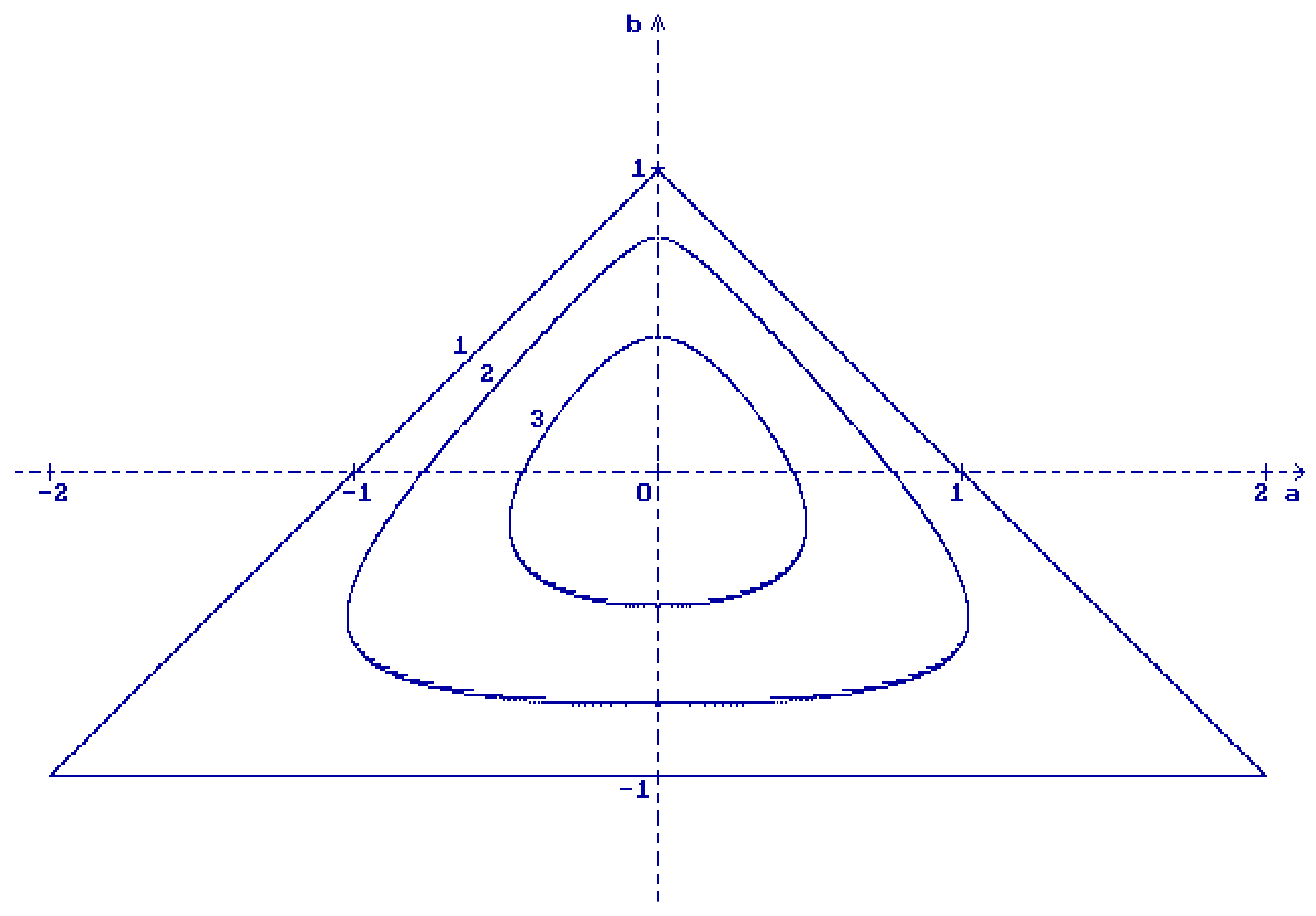
It is known [12] that the necessary and sufficient conditions for asymptotic mean square quasistability of the zero solution of the Equation (25) are

$$\left|b\right|<1,\left|a\right|<1-b,{\sigma }^2<\frac{1+b}{1-b}\left[{(1-b)}^2-a^2\right].$$

(26)

Stability regions defined by the conditions (26) are shown in Figure 1 for different values of ${\sigma }^2$:

(1) ${\sigma }^2=0$; (2) ${\sigma }^2=0.4$; (3) ${\sigma }^2=0.8$.

Consider now the difference equation

$$\begin{array}{c}x(t+h)=ax\left(t\right)+b{\int }_{t-h}^{t}x\left(s\right)ds+\sigma x\left(t\right)\xi (t+h),t>-h,\\ x\left(\theta \right)=\varphi \left(\theta \right),\theta \in \mathsf{\Theta }=[-2h,0],\end{array}$$

(27)

where $h>0$ and all other parameters are the same as in the Equation (25).

In the deterministic case ($\sigma =0$) the characteristic equation of the Equation (27) is

$$e^{\lambda h}=a+\frac{b}{\lambda }(1-e^{-\lambda h}).$$

(28)

Putting $\lambda =i\omega$, $i^2=-1$, transform the Equation (28) to the system of two equations (with respect to a and b)

$$cos\omega h=a+\frac{b}{\omega }sin\omega h,sin\omega h=-\frac{b}{\omega }(1-cos\omega h).$$

(29)

It is easy to show that the system (29) has the following three solutions:

$$\begin{array}{c}a=1,b=-\omega tan\frac{\omega h}{2},\\ a+bh=1,\\ a=cos\omega h+2{cos}^2\frac{\omega h}{2},b=-\omega cot\frac{\omega h}{2}.\end{array}$$

(30)

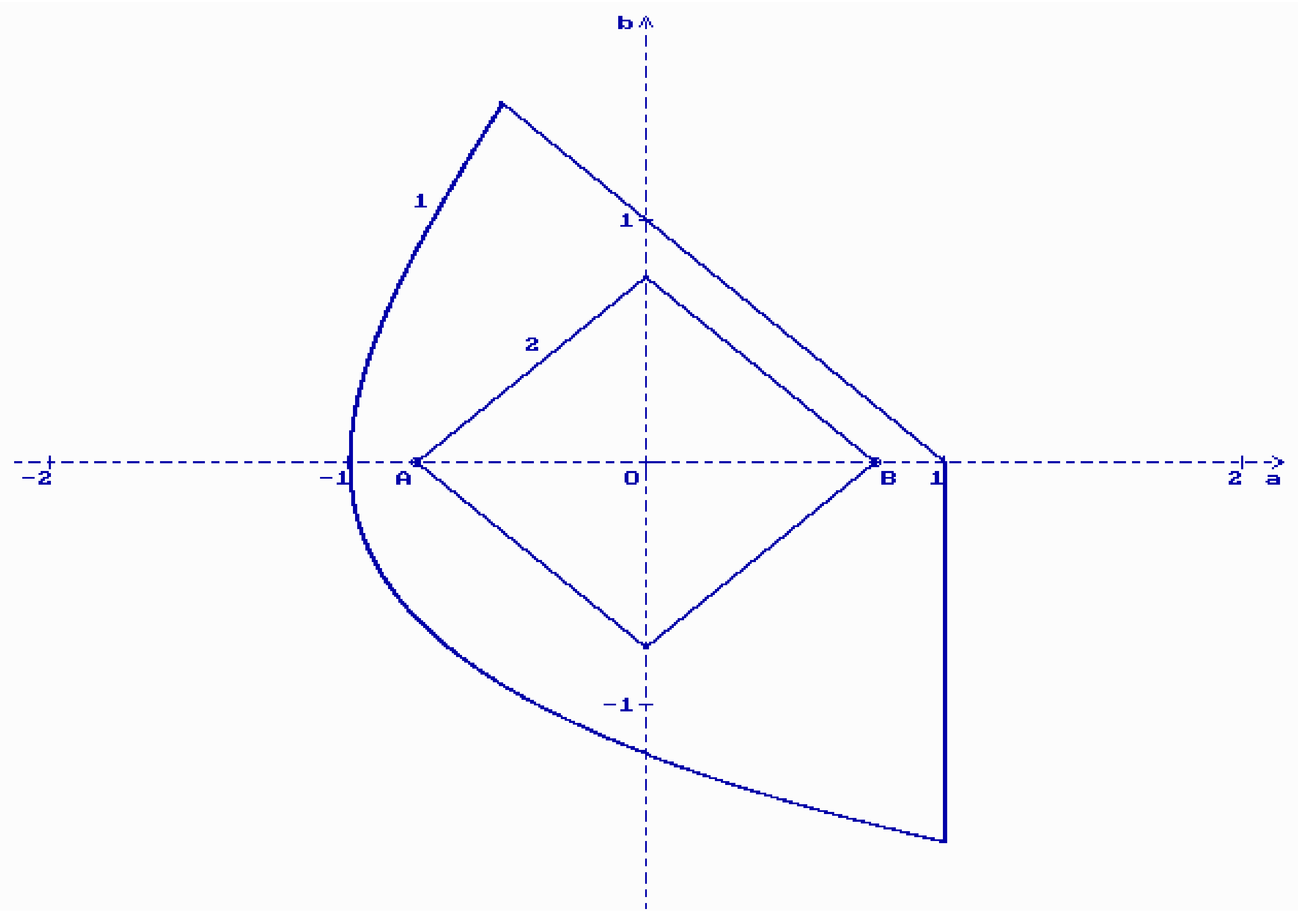
The solutions (30) define the region of asymptotic stability for the zero solution of the Equation (27) if $\sigma =0$. In Figure 2 the corresponding stability region (the bound 1) is shown for $h=1$.

Immediately from (27) it follows $\mathbf{E}{x}^2(t+h)\le \left[\right(\left|a\right|+{\left|b\right|h)}^2+{\sigma }^2]{sup}_{s\le [t-h,t]}\mathbf{E}{x}^2\left(s\right)$. Thus, the inequality

$$\left|a\right|+\left|b\right|h<\sqrt{1-{\sigma }^2}$$

(31)

is a sufficient condition for asymptotic mean square stability of the zero solution of the Equation (27). Corresponding stability region is shown in Figure 2 (the bound 2) for $h=1$, ${\sigma }^2=0.4$.

It is easy to see that the stability region obtained by virtue of the condition (31) (the bound 2) is far enough (even for $\sigma =0$) from the exact stability region (the bound 1).

The unsolved problem is:to get the necessary and sufficient conditions for asymptotic mean square stability of the zero solution of the Equation (27) for $\sigma \ne 0$.

Remark 8.

If $b=0$ then both conditions (26) and (31) coincide and take the form $a^2+{\sigma }^2<1$. It is the necessary and sufficient condition for asymptotic mean square stability of the zero solution of the Equation (27) in the case $b=0$. Thus, the points A and B in Figure 2 with the coordinates $-\sqrt{1-{\sigma }^2}$ and $\sqrt{1-{\sigma }^2}$ respectively belong to the bound of the exact stability region.

4. Stochastic Hyperbolic Equation

Problem 7

Consider the optimal control problem for the stochastic differential equation, containing two-parameter white noise

$$\begin{array}{c}\frac{{\partial }^2\xi \left(z\right)}{\partial x\partial y}=a(z,\xi \left(z\right))+B(z,\xi \left(z\right))u(z,\xi \left(z\right))+b(z,\xi \left(z\right))\frac{{\partial }^{2}w\left(z\right)}{\partial x\partial y},\\ \xi (x,0)=\alpha \left(x\right),\xi (0,y)=\beta \left(y\right),\alpha \left(0\right)=\beta \left(0\right),\end{array}$$

(32)

with the performance criterion

$$J\left(u\right)=\mathbf{E}\left[\mathsf{\Phi }\left(\xi \left(Z\right)\right)+\int {\int }_G{\left|N(z,\xi \left(z\right))u(z,\xi \left(z\right))\right|}^{2}dxdy\right].$$

(33)

Here $z=(x,y)\in G=[0,X]\times [0,Y]$, $Z=(X,Y)$, $\xi \left(z\right)\in {\mathbf{R}}^n$, $a(z,q)\in {\mathbf{R}}^n$, $B(z,q)\in \{{\mathbf{R}}^l\to {\mathbf{R}}^n\}$, $b(z,q)\in \{{\mathbf{R}}^m\to {\mathbf{R}}^n\}$, $N(z,q)\in \{{\mathbf{R}}^l\to {\mathbf{R}}^d\}$, $w\left(z\right)=w(x,y)$ is the n-dimensional two-parameter Wiener process, $u(z,q)\in {\mathbf{R}}^l$ is a control, $q\in {\mathbf{R}}^n$, $\mathbf{E}$ is the expectation. Equations of the type of (32) have been studied, for example, in [17,18].

The optimal control for the problem (32) and (33) has been obtained in [19] via stochastic derivatives [20,21] and Clark’s representation [21]. In particular, from [19] it follows that for the simple scalar case of the problem (32) and (33)

$$\begin{array}{c}\frac{{\partial }^2\xi \left(z\right)}{\partial x\partial y}=u(z,\xi \left(z\right))+\frac{{\partial }^{2}w\left(z\right)}{\partial x\partial y},\\ J\left(u\right)=\mathbf{E}\left[{\xi }^2\left(Z\right)+\int {\int }_G{u}^2(z,\xi \left(z\right))dxdy\right],\end{array}$$

(34)

the obtained optimal control has the form

$$u_0\left(z\right)=\frac{{\mathbf{E}}_z{D}^2\zeta (x,t;s,y)}{{\mathbf{E}}_z{D}^1\zeta (x,y)},$$

(35)

where $D^1\zeta (x,y)$ and $D^2\zeta (x,t;s,y)$ are respectively the first and the second stochastic derivatives of the functional $\zeta \left(Z\right)=e^{\frac{1}{2}(1-{\xi }^2\left(Z\right))}$, ${\mathbf{E}}_z$ is the conditional expectation.

On the other hand the optimal control problem (32) and (33) has been studied by virtue of the necessary condition of control optimality in [22], where, in particular, the optimal control of the problem (34) has been obtained in the form

$$u_0\left(z\right)=\frac{\xi \left(z\right)-{\mathbf{E}}_z[\xi (X,y)+\xi (x,Y)]}{1+(X-x)(Y-y)}.$$

(36)

Remark 9.

For comparison note that in the similar case of the ordinary stochastic differential equation the optimal control of the problem

$$\begin{array}{c}\dot{\xi }\left(t\right)=u\left(t\right)+\dot{w}\left(t\right),\\ J\left(u\right)=\mathbf{E}\left[{\xi }^2\left(T\right)+{\int }_0^T{u}^2\left(t\right)dt\right],\end{array}$$

has the explicit form [23]

$$u_0\left(t\right)=-\frac{\xi \left(t\right)}{1+T-t}.$$

The unsolved problem is:to prove that the both presentations (35) and (36) of the optimal control of the problem (34) coincide and to get the optimal control in the explicit form.

5. Conclusions

When the author was a student, his teacher, the outstanding mathematician and one of the greatest founders of the modern theory of stochastic processes, Iosif Ilyich Gikhman, once said: “To say how difficult or simple this problem is, it is possible only after this problem will be solved”.

Since the problems proposed here have not yet been solved, let us do not say about their complexity. Maybe, for a long time they just did not receive enough attention. The author hopes that the publication of already known unsolved problems, together with problems that have arisen quite recently, will attract more new researchers, both experienced and young, to them. And a time will come when these problems will be solved one by one...

Perhaps, for this, new ideas should appear, entailing not only the solution of the proposed here unsolved problems, but also a new round in the development of the general theory of stochastic processes... Let’s hope...