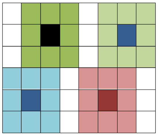
Figure 1.
Octrees of a pixel matrix with size 6 × 8.
Figure 1.
Octrees of a pixel matrix with size 6 × 8.
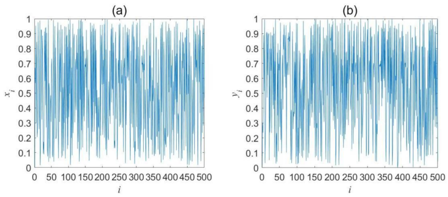
Figure 2.
The trajectories of improved sequences: (a) x-dimensional variable (b) y-dimensional variable.
Figure 2.
The trajectories of improved sequences: (a) x-dimensional variable (b) y-dimensional variable.
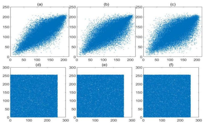
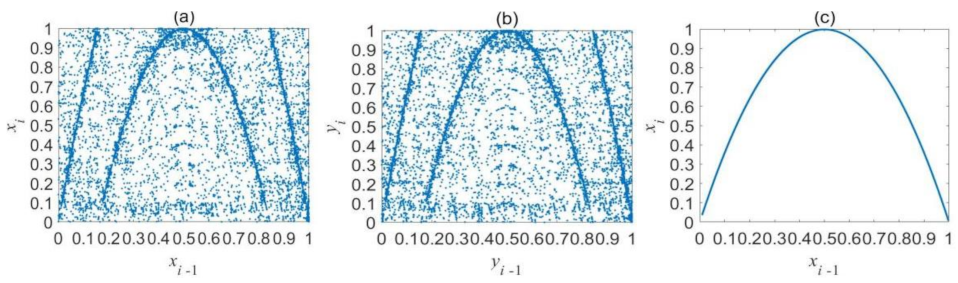
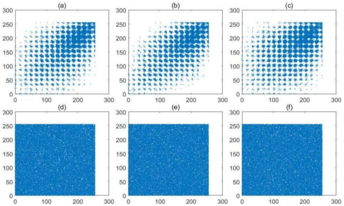
Figure 3.
The phase diagrams: (a) x-dimensional variable of improved sequences (b) y-dimensional variable of improved sequences (c) Equations (1).
Figure 3.
The phase diagrams: (a) x-dimensional variable of improved sequences (b) y-dimensional variable of improved sequences (c) Equations (1).
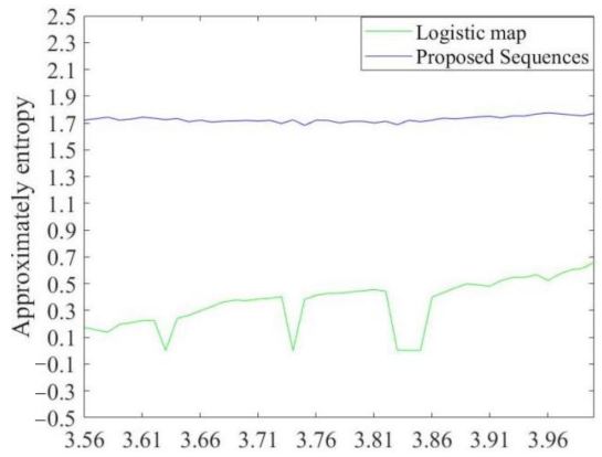
Figure 4.
Approximate entropy of x-dimensional proposed sequence and Equation (1).
Figure 4.
Approximate entropy of x-dimensional proposed sequence and Equation (1).
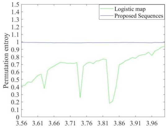
Figure 5.
Permutation entropy of x-dimensional proposed sequence and Equation (1).
Figure 5.
Permutation entropy of x-dimensional proposed sequence and Equation (1).
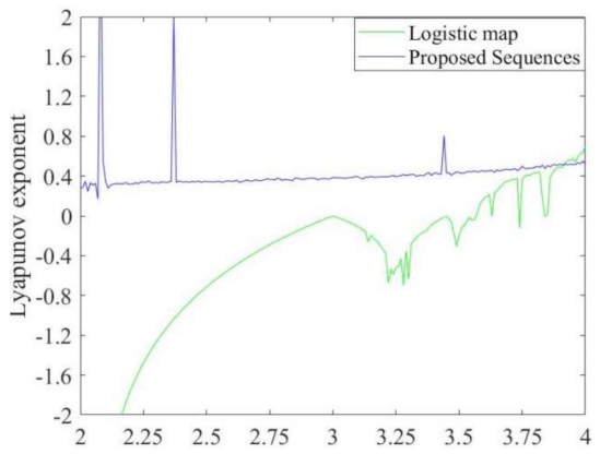
Figure 6.
Lyapunov exponent of x-dimensional proposed sequence and Equation (1).
Figure 6.
Lyapunov exponent of x-dimensional proposed sequence and Equation (1).
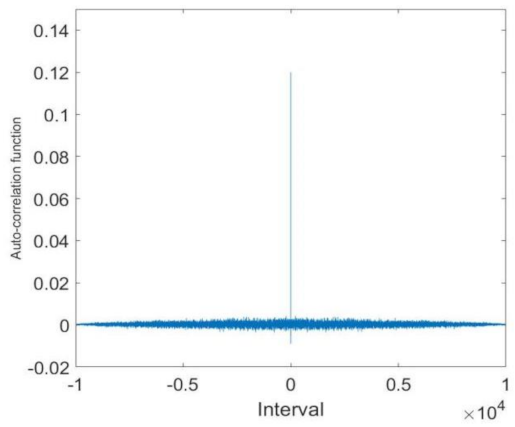
Figure 7.
Auto-correlation function.
Figure 7.
Auto-correlation function.
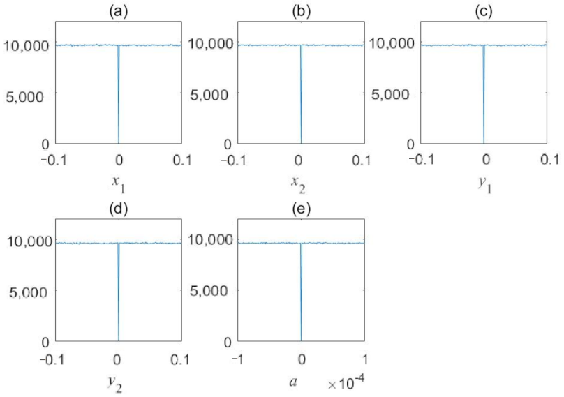
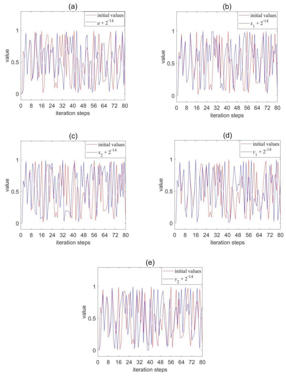
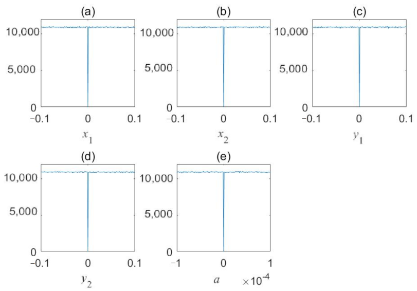
Figure 8.
Sensitivity analysis: (a) The key change is a + 2−14 (b) The key change is x1 + 2−14 (c) The key change is x2 + 2−14 (d) The key change is y1 + 2−14 (e) The key change is y2 + 2−14.
Figure 8.
Sensitivity analysis: (a) The key change is a + 2−14 (b) The key change is x1 + 2−14 (c) The key change is x2 + 2−14 (d) The key change is y1 + 2−14 (e) The key change is y2 + 2−14.
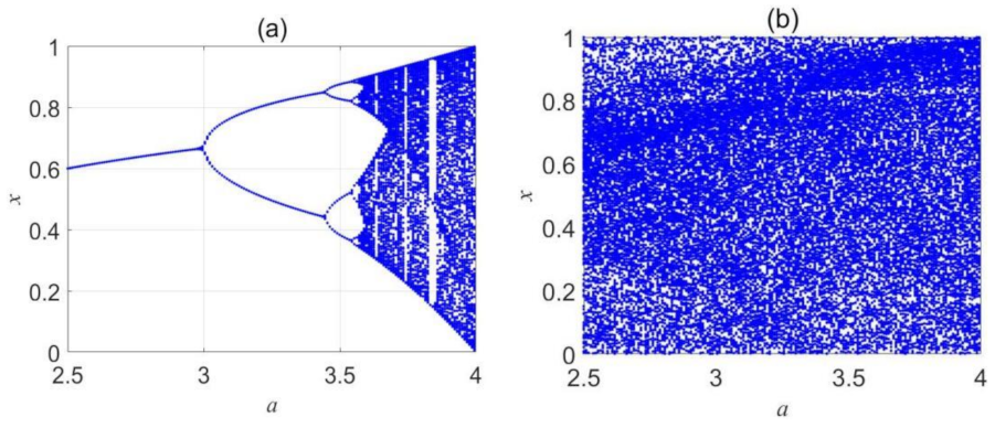
Figure 9.
Bifurcation diagrams: (a) The original chaotic map; (b) The improved chaotic map.
Figure 9.
Bifurcation diagrams: (a) The original chaotic map; (b) The improved chaotic map.
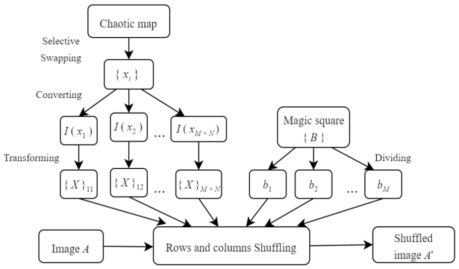
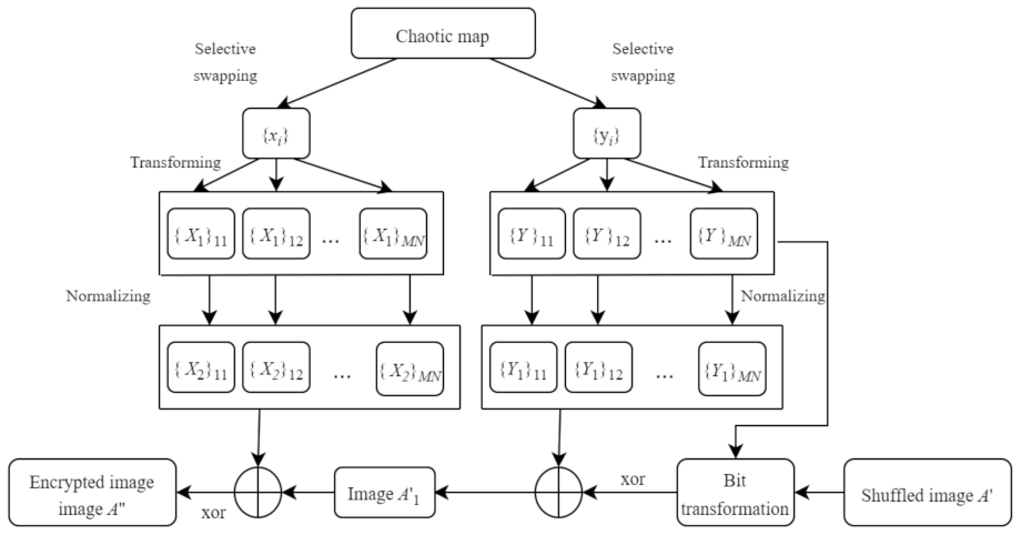
Figure 10.
The flowchart of the shuffling process.
Figure 10.
The flowchart of the shuffling process.
Figure 11.
The flowchart of the substitution process.
Figure 11.
The flowchart of the substitution process.
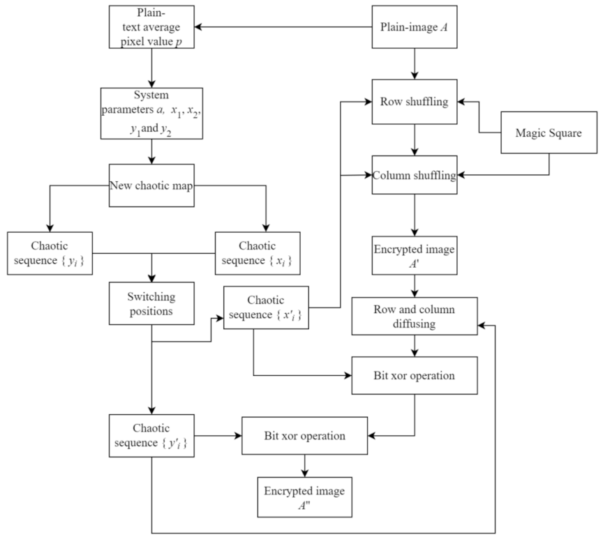
Figure 12.
The flowchart of the image encryption algorithm.
Figure 12.
The flowchart of the image encryption algorithm.
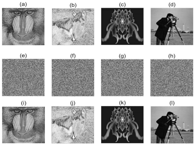
Figure 13.
Encryption and decryption experiments (a–d) Plain-text images; (e–h) Encrypted images; (i–l) Decrypted images with correct keys.
Figure 13.
Encryption and decryption experiments (a–d) Plain-text images; (e–h) Encrypted images; (i–l) Decrypted images with correct keys.
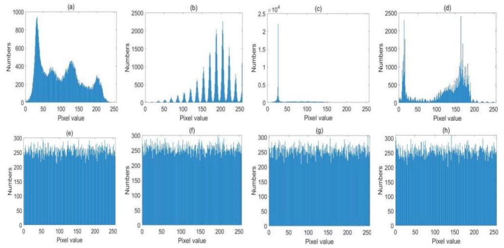
Figure 14.
The histogram analysis: (a–d) Original images: Baboon, Horse, Flower, Cameraman; (e–h) Encrypted images: Baboon, Horse, Flower, Cameraman.
Figure 14.
The histogram analysis: (a–d) Original images: Baboon, Horse, Flower, Cameraman; (e–h) Encrypted images: Baboon, Horse, Flower, Cameraman.
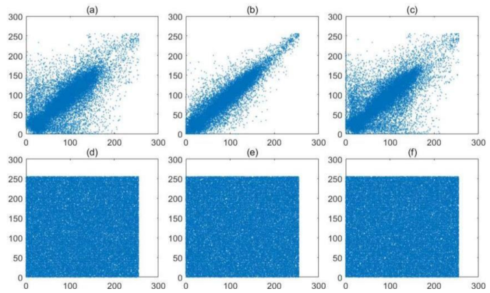
Figure 15.
Correlation analysis of Baboon image: (a) Adjacent pixel points of the plain-text image in horizontal direction; (b) Adjacent pixel points of the plain-text image in vertical direction; (c) Adjacent pixel points of the plain-text image in diagonal direction; (d) Adjacent pixel points of the encrypted image in horizontal direction; (e) Adjacent pixel points of the encrypted image in vertical direction; (f) Adjacent pixel points of the encrypted image in diagonal direction.
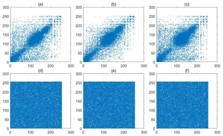
Figure 16.
Correlation analysis of Horse image: (a) Adjacent pixel points of the plain-text image in horizontal direction; (b) Adjacent pixel points of the plain-text image in vertical direction; (c) Adjacent pixel points of the plain-text image in diagonal direction; (d) Adjacent pixel points of the encrypted image in horizontal direction; (e) Adjacent pixel points of the encrypted image in vertical direction; (f) Adjacent pixel points of the encrypted image in diagonal direction.
Figure 17.
Correlation analysis of Flower image: (a) Adjacent pixel points of the plain-text image in horizontal direction; (b) Adjacent pixel points of the plain-text image in vertical direction; (c) Adjacent pixel points of the plain-text image in diagonal direction; (d) Adjacent pixel points of the encrypted image in horizontal direction; (e) Adjacent pixel points of the encrypted image in vertical direction; (f) Adjacent pixel points of the encrypted image in diagonal direction.
Figure 18.
Correlation analysis of Cameraman image: (a) Adjacent pixel points of the plain-text image in horizontal direction; (b) Adjacent pixel points of the plain-text image in vertical direction; (c) Adjacent pixel points of the plain-text image in diagonal direction; (d) Adjacent pixel points of the encrypted image in horizontal direction; (e) Adjacent pixel points of the encrypted image in vertical direction; (f) Adjacent pixel points of the encrypted image in diagonal direction.
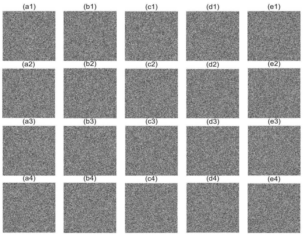
Figure 19.
Decrypted images with only 10−10 difference in the secret keys (a1–e1): Baboon cipher images with a + 10−10, x1 + 10−10, x2 + 10−10, y1 + 10−10, y2 + 10−10; (a2–e2): Horse cipher images with a + 10−10, x1 + 10−10, x2 + 10−10, y1 + 10−10, y2 + 10−10; (a3–e3): Flower cipher images with a + 10−10, x1 + 10−10, x2 + 10−10, y1 + 10−10, y2 + 10−10; (a4–e4): Cameraman cipher images with a + 10−10, x1 + 10−10, x2 + 10−10, y1 + 10−10, y2 + 10−10.
Figure 20.
MSE analysis of encryption process of Baboon image: (a) x1; (b) x2; (c) y1; (d) y2; (e) a.
Figure 20.
MSE analysis of encryption process of Baboon image: (a) x1; (b) x2; (c) y1; (d) y2; (e) a.
Figure 21.
MSE analysis of decryption process of Baboon image: (a) x1; (b) x2; (c) y1; (d) y2; (e) a.
Figure 21.
MSE analysis of decryption process of Baboon image: (a) x1; (b) x2; (c) y1; (d) y2; (e) a.
Figure 22.
Robustness analysis (a1) 1% speckle noise (encrypted); (a2) 1% speckle noise (decrypted); (b1) 3% speckle noise (encrypted); (b2) 3% speckle noise (decrypted); (c1) 5% data loss (encrypted); (c2) 5% data loss (decrypted); (d1) 10% data loss (encrypted); (d2) 10% data loss (decrypted).
Figure 22.
Robustness analysis (a1) 1% speckle noise (encrypted); (a2) 1% speckle noise (decrypted); (b1) 3% speckle noise (encrypted); (b2) 3% speckle noise (decrypted); (c1) 5% data loss (encrypted); (c2) 5% data loss (decrypted); (d1) 10% data loss (encrypted); (d2) 10% data loss (decrypted).
Table 1.
The 16-order magic square.
Table 1.
The 16-order magic square.
| 256 | 2 | 3 | 253 | 252 | 6 | 7 | 249 | 248 | 10 | 11 | 245 | 244 | 14 | 15 | 241 |
| 17 | 239 | 238 | 20 | 21 | 235 | 234 | 24 | 25 | 231 | 230 | 28 | 29 | 227 | 226 | 32 |
| 33 | 223 | 222 | 36 | 37 | 219 | 218 | 40 | 41 | 215 | 214 | 44 | 45 | 211 | 210 | 48 |
| 208 | 50 | 51 | 205 | 204 | 54 | 55 | 201 | 200 | 58 | 59 | 197 | 196 | 62 | 63 | 193 |
| 192 | 66 | 67 | 189 | 188 | 70 | 71 | 185 | 184 | 74 | 75 | 181 | 180 | 78 | 79 | 177 |
| 81 | 175 | 174 | 84 | 85 | 171 | 170 | 88 | 89 | 167 | 166 | 92 | 93 | 163 | 162 | 96 |
| 97 | 159 | 158 | 100 | 101 | 155 | 154 | 104 | 105 | 151 | 150 | 108 | 109 | 147 | 146 | 112 |
| 144 | 114 | 115 | 141 | 140 | 118 | 119 | 137 | 136 | 122 | 123 | 133 | 132 | 126 | 127 | 129 |
| 128 | 130 | 131 | 125 | 124 | 134 | 135 | 121 | 120 | 138 | 139 | 117 | 116 | 142 | 143 | 113 |
| 145 | 111 | 110 | 148 | 149 | 107 | 106 | 152 | 153 | 103 | 102 | 156 | 157 | 99 | 98 | 160 |
| 161 | 95 | 94 | 164 | 165 | 91 | 90 | 168 | 169 | 87 | 86 | 172 | 173 | 83 | 82 | 176 |
| 80 | 178 | 179 | 77 | 76 | 182 | 183 | 73 | 72 | 186 | 187 | 69 | 68 | 190 | 191 | 65 |
| 64 | 194 | 195 | 61 | 60 | 198 | 199 | 57 | 56 | 202 | 203 | 53 | 52 | 206 | 207 | 49 |
| 209 | 47 | 46 | 212 | 213 | 43 | 42 | 216 | 217 | 39 | 38 | 220 | 221 | 35 | 34 | 224 |
| 225 | 31 | 30 | 228 | 229 | 27 | 26 | 232 | 233 | 23 | 22 | 236 | 237 | 19 | 18 | 240 |
| 16 | 242 | 243 | 13 | 12 | 246 | 247 | 9 | 8 | 250 | 251 | 5 | 4 | 254 | 255 | 1 |
Table 2.
Adjacent pixel position annotation.
Table 2.
Adjacent pixel position annotation.
| a1 = a(i−1)(j−1) | a8 = a(i−1)j | a7 = a(i−1)(j+1) |
| a2 = ai(j−1) | aij | a6 = ai(j+1) |
| a3 = a(i+1)(j−1) | a4 = a(i+1)j | a5 = a(I + 1)(j+1) |
Table 3.
Variance comparison results.
Table 3.
Variance comparison results.
| Algorithm | Images | Variance |
|---|
| | | Original | Encrypted | Decrypted |
| Proposed | Baboon | 57,916 | 255.3569 | 57,916 |
| | Horse | 189,049 | 223.5373 | 189,049 |
| | Flower | 1,969,923 | 275.9059 | 1,969,923 |
| | Cameraman | 124,091 | 286.8784 | 124,091 |
| | Baboon | 57,916 | 255.3569 | 57,916 |
| Patro, K. A. K .et al. [26] | Cameraman | 110,970 | 250.4141 | 110,970 |
| Patro, K. A. K. et al. [27] | Cameraman | 110,970 | 259.1328 | 110,970 |
| Tsafack, N. et al. [28] | Baboon | 753,712.8784 | 909.4980 | - |
| Patro, K. A. K. et al. [29] | Cameraman | 110,970 | 334.5391 | - |
| Patro, K. A. K. et al. [30] | Cameraman | 110,970 | 298.1875 | 110,970 |
Table 4.
The Chi-square test results.
Table 4.
The Chi-square test results.
| Algorithms | Images | χ2 Test | Testing Results | |
|---|
| χ22550.05 = 293.2478 | χ22550.01 = 310.457 |
|---|
| Proposed | Baboon | 254.3594 | Pass | Pass |
| | Horse | 222.6641 | Pass | Pass |
| | Flower | 274.8281 | Pass | Pass |
| | Cameraman | 285.7578 | Pass | Pass |
| Patro, K.A. K. et al. [31] | Baboon | 225.3438 | Pass | |
| Yang, F. et al. [32] | Baboon (512 × 512) | 265.4 | Pass | |
Table 5.
Correlation coefficient analysis.
Table 5.
Correlation coefficient analysis.
| Images | Horizontal | Vertical | Diagonal |
|---|
| Baboon image | 0.8502 | 0.8174 | 0.7646 |
| Encrypted Baboon | 0.0002 | 0.0038 | −0.0007 |
| Horse image | 0.6425 | 0.6682 | 0.5179 |
| Encrypted Horse | 0.0027 | −0.0051 | −0.0030 |
| Flower image | 0.8862 | 0.9613 | 0.8772 |
| Encrypted Flower | 0.0025 | 0.0025 | 0.0013 |
| Cameraman image | 0.9333 | 0.9569 | 0.9052 |
| Encrypted Cameraman | 0.0055 | −0.0065 | −0.0024 |
| Patro, K. A. K. et al. [26] Cameraman | −0.0013 | 0.0017 | 0.0070 |
| Patro, K. A. K. et al. [27] Baboon | 0.0029 | 0.0003 | −0.0020 |
| Patro, K. A. K. et al. [31] Baboon | 0.0003 | −0.0002 | −0.0017 |
Table 6.
Key space.
| Algorithms | Key Space |
|---|
| Proposed | 2233 |
| Tang, J. et al. [5] | 2231 |
| Zhang, Y. P. et al. [33] | 2.6 × 10²³ |
| Li, R. Z. et al. [34] | 2200 |
| Liu, Y. et al. [35] | 2186 |
| Chen, C. et al. [36] | 2135 |
| Liao, X. et al. [37] | 2194 |
| Patro, K. A. K. et al. [38] | 1.2446 × 2327 |
Table 7.
Information entropy.
Table 7.
Information entropy.
| | Original Image | Encrypted Image |
|---|
| Baboon | 7.2436 | 7.9972 |
| Horse | 6.5645 | 7.9976 |
| Flower | 5.5145 | 7.9970 |
| Cameraman | 7.0084 | 7.9968 |
| Yang, Y. et al. [39] Cameraman | - | 7.9970 |
| Kaur, G. et al. [40] Baboon | 7.7067 | 7.9852 |
| Kaur, G. et al. [40] Cameraman | 7.0097 | 7.9846 |
Table 8.
Local entropy.
| | Original Image | Encrypted Image |
|---|
| Baboon | 6.787927 | 7.9020763 |
| Flower | 5.159931 | 7.902534 |
| Horse | 6.294101 | 7.901957 |
| Cameraman | 5.166450 | 7.901997 |
| Kaur, G. et al. [40] Cameraman | - | 7.8822 |
| Kaur, G. et al. [40] Baboon | - | 7.8945 |
| El-Latif, A. A. A. et al. [42] Rustic | 5.44114 | 7.90284 |
Table 9.
The values of NPCR and UACI.
Table 9.
The values of NPCR and UACI.
| Algorithms | NPCR | UACI |
|---|
| Baboon | 0.9963 | 0.3344 |
| Horse | 0.9961 | 0.3347 |
| Flower | 0.9964 | 0.3365 |
| Cameraman | 0.9962 | 0.3344 |
| Toktas, A. and Erkan, U. [23] Cameraman | 0.9961 | 0.3347 |
| Patro, K.A. K. et al. [27] Cameraman | 0.9962 | 0.3344 |
| Yang, Y. et al. [39] Cameraman | 0.9963 | 0.3341 |
| Patro, K. A. K. et al. [43] Baboon (512 × 512) | 0.9961 | 0.3347 |
| Sravanthi, D. et al. [44] Cameraman | 0.9961 | 0.3342 |
Table 10.
Speed tests.
| Algorithms | Images | Unit (s) | Speed (Mb/s) |
|---|
| Proposed | Baboon | 0.6087 | 0.8214 |
| | Horse | 0.6033 | 0.8287 |
| | Flower | 0.5957 | 0.8393 |
| | Cameraman | 0.6021 | 0.8304 |
| Khan, J. S. and Ahmad, J. [46] | Flower | 0.55 | - |
| Ayoup, A. M. et al. [47] | Flower | 7.21 | - |


