Abstract
In this paper, a multi-server retrial queue with two orbits is considered. There are two arrival processes of positive customers (with two types of customers) and one process of negative customers. Every positive customer requires some amount of resource whose total capacity is limited in the system. The service time does not depend on the customer’s resource requirement and is exponentially distributed with parameters depending on the customer’s type. If there is not enough amount of resource for the arriving customer, the customer goes to one of the two orbits, according to his type. The duration of the customer delay in the orbit is exponentially distributed. A negative customer removes all the customers that are served during his arrival and leaves the system. The objects of the study are the number of customers in each orbit and the number of customers of each type being served in the stationary regime. The method of asymptotic analysis under the long delay of the customers in the orbits is applied for the study. Numerical analysis of the obtained results is performed to show the influence of the system parameters on its performance measures.
1. Introduction
The theory of queuing systems with repeated calls (Retrial Queue) is an important section of the modern teletraffic theory, the relevance of which is due to wide practical applications, such as the performance evaluation and design of broadcast, radio, and cellular networks, as well as local networks with the random multiple access protocols. In the monographs [1,2,3], the detailed survey of recent queuing models applications in telecommunication, modern computer networks, and information systems are presented.
The retry phenomenon is the integral feature of data transmission systems, and this phenomenon ignored in theoretical research can lead to significant errors in engineering decisions. Many multimedia and service applications on subscriber devices can automatically generate such requests, without any relative restrictions. Such unaccounted traffic consumes the channel resource in excess of the planned one. On the network sections, overflows begin to appear, that leads to the service rejection; thus, it generates more repeated calls again.
A large number of publications has been devoted to the study of retrial queues. The most extensive reviews of significant results, up to 2008, are presented in the monographs [4,5].
Queuing models with negative customers [6,7,8], or G-queues, are useful models for the analysis of multiprocessor computer systems, neural networks, communication systems, and manufacturing [9,10]. In its simplest version, a negative customer (negative arrival) has the effect of a positive (ordinary) customer(s) being deleted according to some strategy. For example:
- a negative arrival eliminates all the customers in the system or in its part, e.g., under the service or in the buffer (catastrophes);
- a negative arrival removes a customer from the system, e.g., from the server, from the head of the queue, or its end;
- a negative arrival breaks the service device, etc.
Negative arrivals are interpreted as viruses, orders or inhibitor signals, etc. The detailed overview of G-queues is presented in Reference [11]. Retrial queuing systems with negative arrivals have been considered, for example, in References [12,13,14,15]. The effects of negative customers considered in these papers are close to the effect of breakdowns. Retrial queues with breakdowns have been studied in References [16,17,18,19].
Other features of modern data transmission systems are random amounts of transmitted data and requests for additional resources. Often, in telecommunication systems, calls come from different sources and have different service time characteristics and different priorities, or they need more than one service device, etc. These features make the system analysis more complex. Identifying these aspects and analyzing their influence on the systems allow to optimize networks for loss reduction. Such mathematical models are called queuing systems with a random volume of the customers or resource queuing systems [20,21,22,23,24,25,26,27,28]. Resource queuing systems are applied in modern wireless communication networks, cloud computing systems, technical devices, or next-generation data transmission networks. It is known that, in classical queuing theory, the evaluation of almost all performance characteristics leads us to the analysis of a stochastic process of the number of customers in the system. However, it is insufficient if we would like to determine a buffer space capacity of a communication network’s node which guarantees small losses of transmitted data [20,21,23]. Incoming customers can request some resources (for example, the amount of memory). The requests may be random or deterministic. In queuing models, the total amount of resource is usually limited by a constant value , which is called the buffer space capacity of the system. The buffer space is occupied by a customer at the arrival epoch and is entirely released at the service finish epoch. If value R is finite, it leads to additional losses of customers. The complexity of the study of resource systems is due to an universal approach does not exist. We use asymptotic methods [15,27,29], which give asymptotic expressions of the studied system characteristics that are acceptable for practical usage. A retrial queuing system with limited processor sharing (close to resource systems) is considered in Reference [30].
In the paper, the model under study is a non-classical retrial queuing system with non-homogeneous customers. The main feature of the research is the consideration of possible failures in the system. In the paper, we apply the theory of G-queues [6] for modeling breakdowns in real networks. A breakdown is represented by negative customers arriving at the queuing system and removing all served customers if any is present. So, we research the queuing system with all mentioned above features: repeated calls, negative customers, and resource. Such a model can be applied, for example, for 5G New Radio systems. The key feature and the main problem of the 5G New Radio network is that people themselves, cars, buildings, etc., are signal blockers, which is the cause of service interruptions. In this reasoning, the scientific community has the task of analyzing the performance of these systems and improving it in the future. Currently, there are known studies of “basic” mathematical models of such networks. However, due to introducing this technology into the daily lives of subscribers, we need to propose and analyze of the most appropriate mathematical models.
The considered mathematical model is described in Section 2. In Section 3, the method of asymptotic analysis is proposed and applied for the study. The numerical analysis is presented in Section 4. It includes a comparison of asymptotic and simulated distributions, numerical examples for various values of the model parameters, and calculation of some performance characteristics, such as the probability of the first time rejecting (or, in other words, it is a joining probability) and buffer space utilization. The problems and discussions about the applicability of the obtained approximations are presented in the conclusion.
2. Mathematical Model
Let us consider the multi-server retrial queue (Figure 1) with two positive and one negative arrival processes. We call customers arrived in the k-th positive arrival process customers of the k-th type (). All the processes are Poisson with parameters , (for the first and the second type of positive customers), and (for the negative ones). Positive customers need the service, and the service laws are exponential with parameters and for the first and the second type of customers, respectively. In addition, each positive customer requires a deterministic amount of resource ( or , respectively); therefore, a customer occupies some amount of resources during his service. The service time does not depend on customer’s resource requirement. The service unit has a limited capacity of resources, which equals to R. The number of servers N is limited but large enough. If the customer cannot be served at the arrival moment (there is not enough amount of the resource), it goes to the corresponding orbit (some virtual place). The duration of the customers delay in the orbits is distributed exponentially with parameters and , respectively. The negative customer deletes all customers being served in the service unit at his moment of arrival.
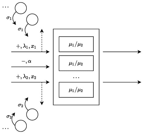
Figure 1.
Resource retrial queue with two orbits and negative customers.
The goal of the paper is to study four-dimensional stochastic process
where is the number of k-type customers in the service unit at the moment t, and is the number of customers in the k-th orbit at the moment t. Then, the state space has the form:
where is a value of the process , and is a value of the process , where .
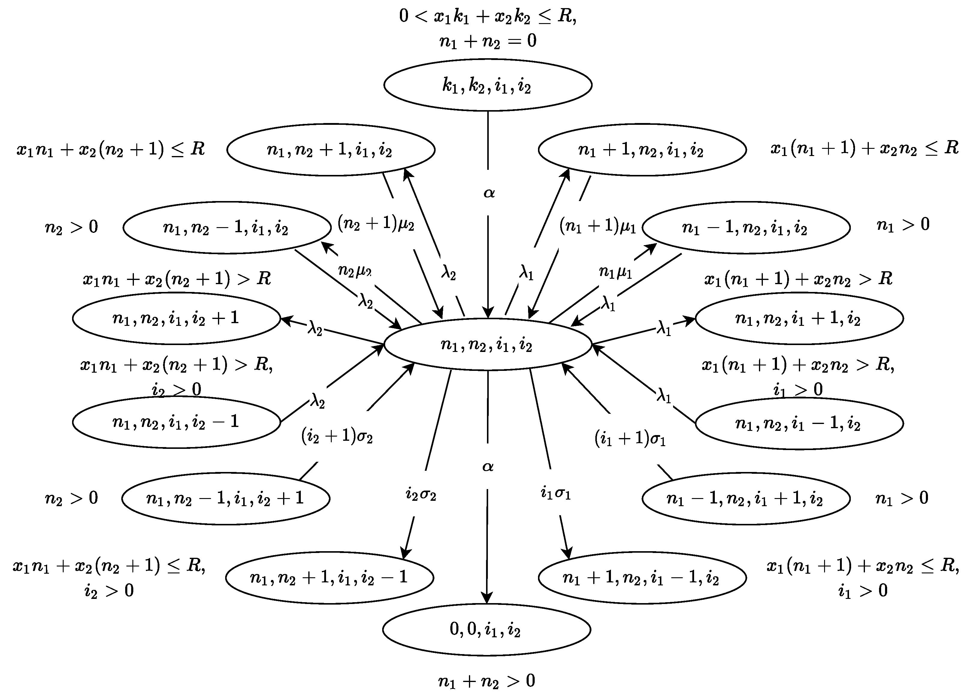
Traditionally, continuous-time Markov chains can be represented as a transition graph. In Figure 2, we depict such a graph for the considered Markov chain . The ovals on the graph represent the states, and the arrows show the possible transitions and their intensities. In addition, next to each state, we show the condition under which it exists, knowing that the central state (any state) on the graph is .
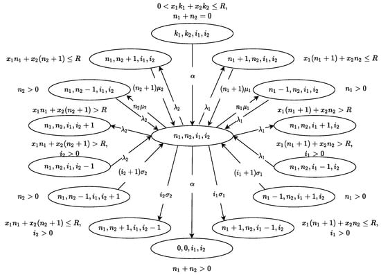
Figure 2.
Graph of the input/output transitions of central state.
Let us consider in more detail the possible events that cause a change in the state of the considered Markov chain:
- the negative customer arrival with intensity , so the number of customers from both types being serviced becomes equal to 0 (transitions and );
- the first type arrival with intensity :
- -
- if there is a sufficient resource amount for the customer, it gets serviced; therefore, the number of customers of the first type being serviced increases by 1 (transitions and );
- -
- otherwise, the customer goes to the orbit and waits for the retrial; therefore, the number of customers in the first orbit increases by 1 (transitions and );
- the end of first type customer service with an intensity ; therefore, the number of customers of the first type being serviced is reduced by 1 (transitions and );
- the successful retrial to service of the first type customer with an intensity ; therefore, the number of customers in the first orbit is reduced by 1, and the number of customers of the first type being serviced is reduced by 1 (transitions and );
- similarly, we have transitions for the second type customers.
So, we will find the stationary probabilities
Let us write the following system of equations for them:
where
From System (1), we write several equations for different states.
- (a)
- For
- (b)
- For
- (c)
- For
- (d)
- For
- (e)
- For
Because of , Equations (a)–(e) have infinite dimension. So, for solving of difference equations System (a)–(e), we use the method of characteristic transforms. This method allows to find solutions of complex equations in queuing theory in more simple way. In the paper, we introduce the following partial characteristic functions:
where .
Note that is a characteristic function of the two-dimensional process of the number of customers in the orbits.
Using Notation (2), Equations (a)–(e) are rewritten as follows:
- (a)
- For
- (b)
- For
- (c)
- For
- (d)
- For
- (e)
- For
Let us denote the matrix . So, the following equation can be written:
where are the followings operators:
Operator is the sum of equations for all values of , . Obviously,
So, we have the following equation:
3. Asymptotic Analysis Method
Since it is not possible to find an explicit form of the solution of equations system (3) and (4), we propose the asymptotic analysis method [15,27,29]. In the paper, we will use the asymptotic condition of the long delay (when and ). The practical mean of the long delay condition is that the service time is much less than the time of repeated call.
The algorithm of the proposed method includes the following steps.
- 1.
- Deriving of the asymptotic mean of the considered process:
- (a)
- introducing of an infinitesimal parameter and an asymptotic function notation (5);
- (b)
- (c)
- deriving of a limit solution of the asymptotic equations for ;
- (d)
- using the inverse substitutions, we obtain the form of the first-order asymptotic characteristic function (10), which gives the value of the asymptotic mean of the considered process.
- 2.
- Deriving of the asymptotic variance of the considered process:
- (a)
- using the result of the first-order asymptotic analysis 1.(d), we rewrite the characteristic function as (11);
- (b)
- (c)
- introducing of an infinitesimal parameter and new asymptotic function notation (13);
- (d)
- rewriting of equations obtained in 2.(b) for the asymptotic notations;
- (e)
- approximating asymptotic functions by its 2th-degree Maclaurin series with respect to as (14);
- (f)
- deriving of a limit solution of the asymptotic equations for ;
- (g)
- using the inverse substitutions, we obtain the form of the second-order asymptotic characteristic function, which gives the value of the asymptotic variance of the considered process.
- 3.
- Combining the results of 1.(d) and 2.(g), we obtain the final form of asymptotic characteristic function (21).
3.1. First-Order Asymptotics
First of all, we denote , where and . In the first-order asymptotic analysis method, we use the following notations:
where is infinitesimal, and is an asymptotic function.
Substituting Notations (5) into Equations (3) and (4), we obtain the following asymptotic equations:
Let us make limits . Then, System (6) has the form:
Obviously, the solution of Equation (7) has the form
where is the matrix of the stationary probabilities of the states of process ; , are normalized means of the number of customers in the orbit, which are calculated from the following equations (obtained by substituting (8) in (7)):
After returning to Substitutions (5), we have obtained the first-order approximation of the characteristic function
where and are normalized means of processes and .
3.2. Second-Order Asymptotics
The first step of the second-order asymptotic analysis is rewriting the characteristic functions using the result of the first-order asymptotics (10) as follows:
where is matrix of characteristic functions of two-dimensional stochastic centered process .
The next step of the analysis is introducing the following notations (as in Section 3.1):
The solution of System (14) will be found in the following multiplicative form:
where is an unknown scalar function, and , are unknown operators, which will be found further.
Make some transformations and obtain .
The solution of System (16) has the form:
where and are normalized variances of the stochastic process , and is their normalized covariance. For the , , and finding, we substitute (17) into System (16):
For (18) solving, let us write the factors for different powers of :
The system of the first and second equations in (19) is the heterogeneous system of linear algebraic equations with respect to and . The determinant of the matrix of the system is equal to zero, while the rank of the extended matrix is equal to the rank of the matrix of coefficients, i.e., the system has many solutions. Comparing the first and second equations of systems (19) and the first equation of (9) (in the first-order asymptotics), we can write:
where
So, we have the following system for and finding:
After returning to Substitutions (13), we obtain that the second-order approximation of the characteristic function has the following form:
So, the asymptotic characteristic function of the considered multi-dimensional process has the following matrix form:
Therefore, two-dimensional process of number of customers in the orbits is asymptotically Gaussian with means’ vector and covariance matrix
4. Numerical Examples
In this section, we present the comparison of asymptotic and simulated distributions for some values of the model parameters. In addition, some performance characteristics of the model are evaluated.
For the numerical examples presentation, we assume the following values of the retrial queue parameters:
We have software applications for the considering model simulation and computing the asymptotic results.
We use the discrete-event simulation. The state of the system is changed by events, such as:
- the arrival of the first customer,
- the arrival of the second customer,
- the arrival of the negative customer,
- the service end of the first customer,
- the service end of the second customer,
- the customer attempt to access the service unit from the first orbit, and
- the customer attempt to access the service unit from the second orbit.
The condition for stopping the simulation is the service end at least customers of each arrival process.
Note that the structural parameters of the system, such as , can take any values, and, with growth R regarding , the number of system states increases, which entails an increase in the time spent on analytical calculating the probability distribution. The proposed parameter values allow for clearly demonstrating the dimension of the system and the influence of the system load parameters, such as , on the main performance characteristics.
First, we compare asymptotic and simulated distributions for various values of (the infinitesimal variable of the asymptotic analysis). In Figure 3, the two-dimensional asymptotic probability distribution of the number of customers in orbits is presented for .
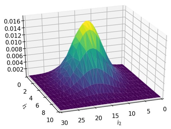
Figure 3.
The two-dimensional asymptotic probability distribution of the number of customers in the orbits.
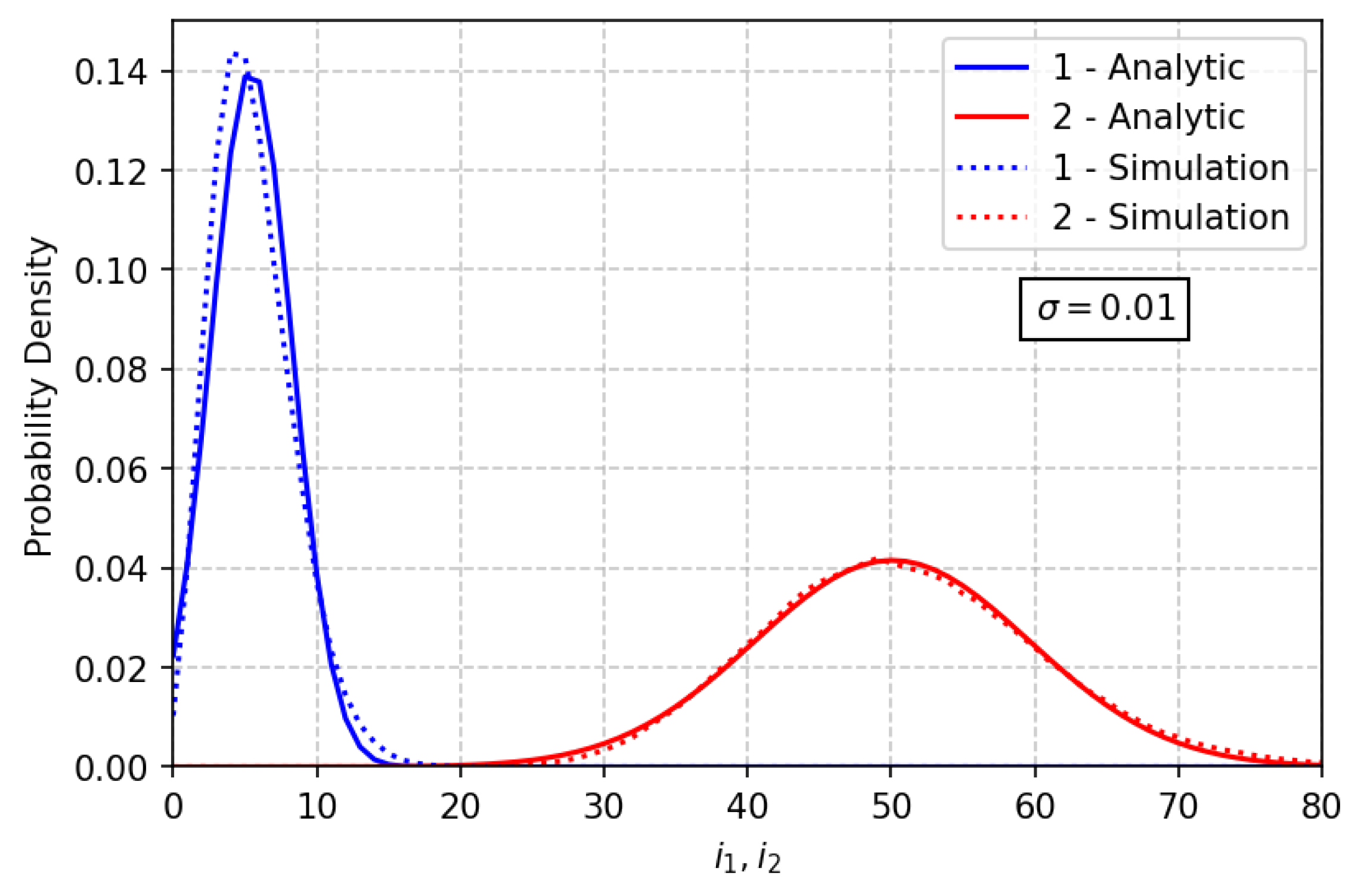
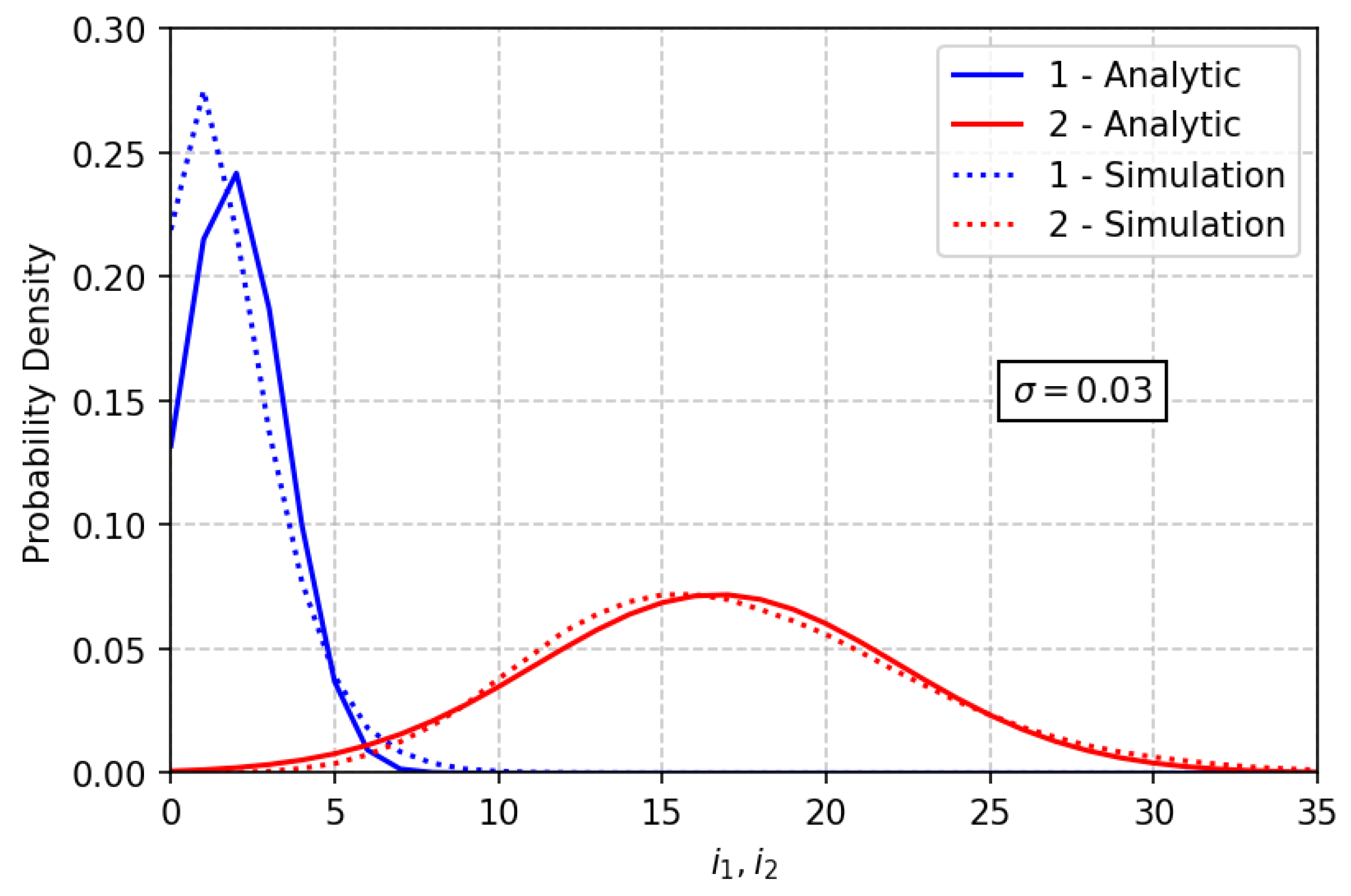
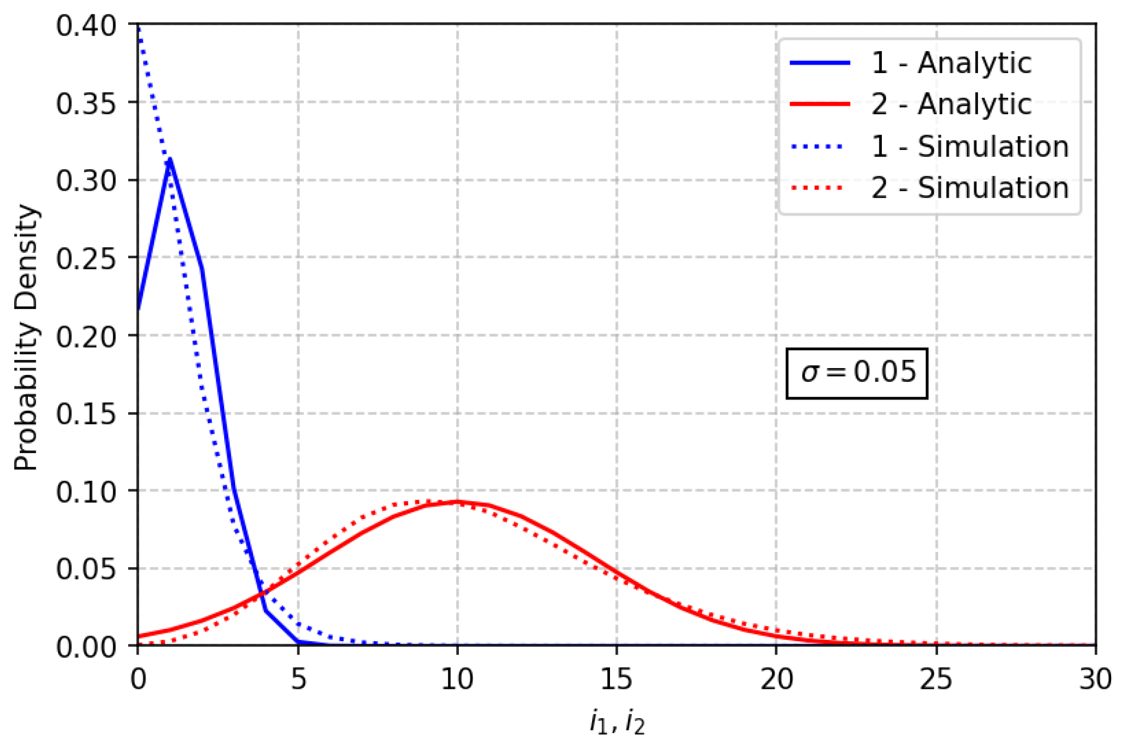
In Figure 4, Figure 5 and Figure 6, you may find the comparison of the asymptotic and simulated one-dimensional distributions for various values of . Curves 1 and 2 are the probability distributions of the number of customers in the first and the second orbits, respectively.
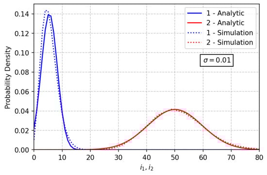
Figure 4.
Comparison of the asymptotic and simulated distributions for .
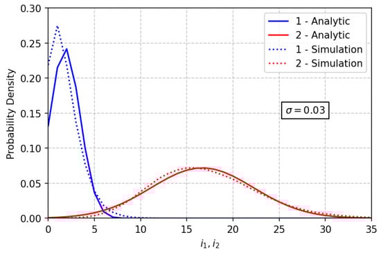
Figure 5.
Comparison of the asymptotic and simulated distributions for .
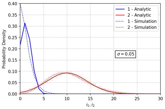
Figure 6.
Comparison of the asymptotic and simulated distributions for .
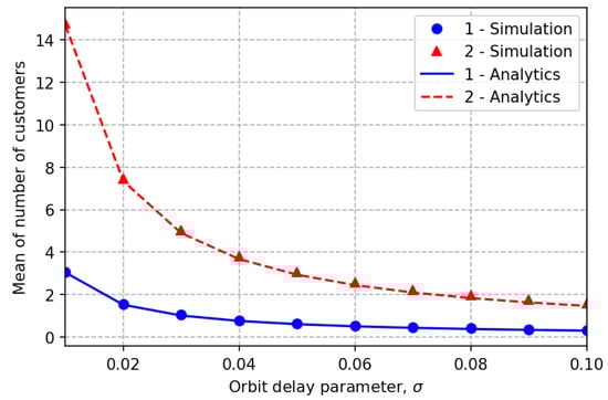
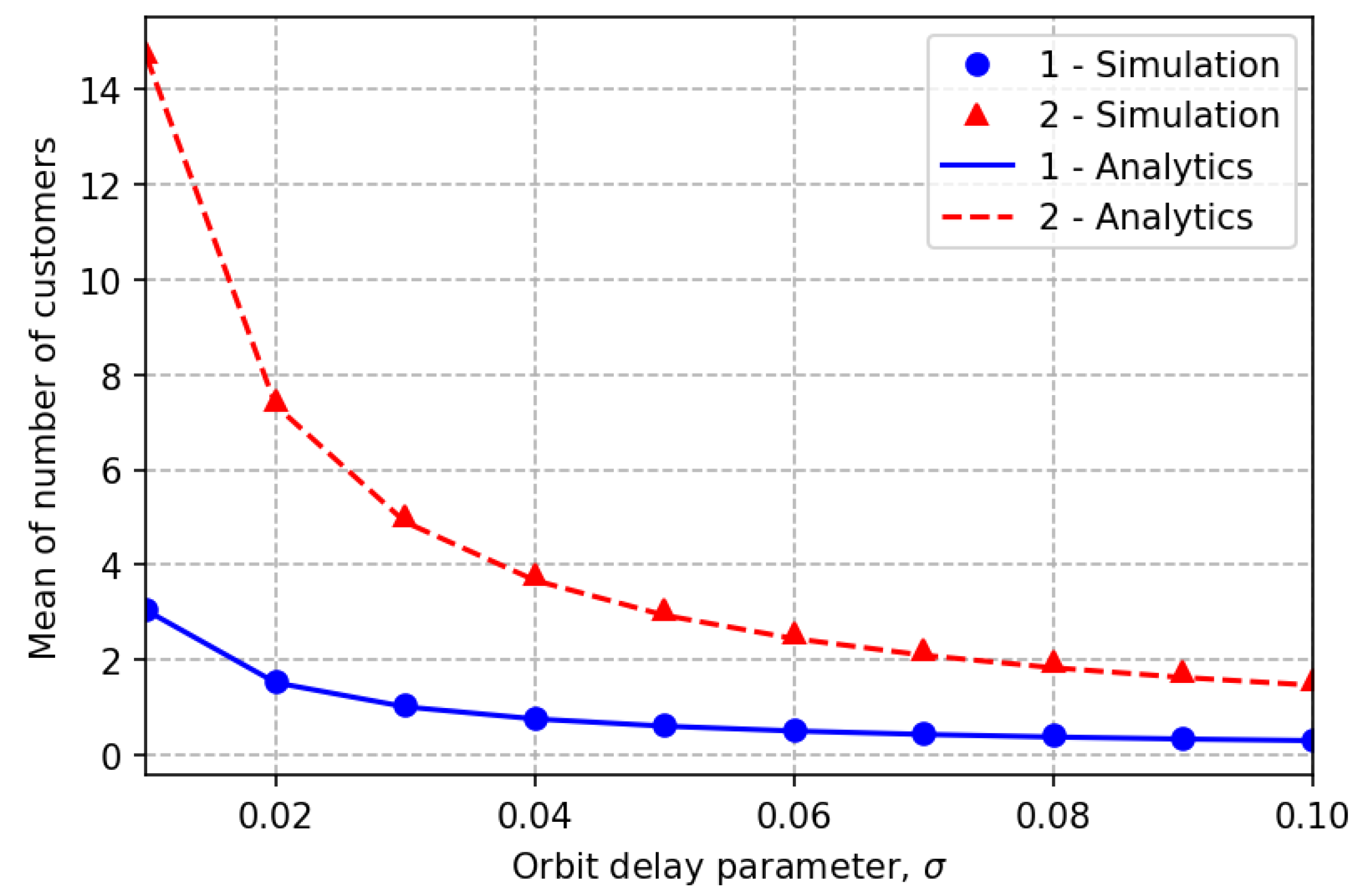
Figure 7.
Asymptotic and simulate means.
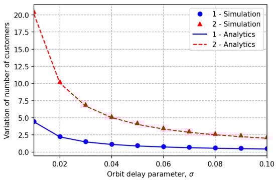
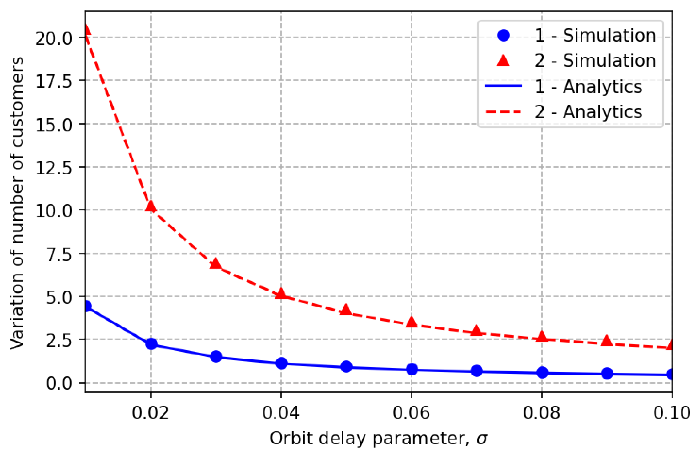
Figure 8.
Asymptotic and simulate variances.
In addition, the relative errors of the asymptotic means and variances (in comparison with the simulated results) are computed (Table 1 and Table 2).

Table 1.
Table of relative errors of means.
Table 2.
Table of relative errors of variances.
Another measure of distributions comparison is Kolmogorov distance
where is the probability distribution of the processes or calculated using the asymptotic formula, and is the corresponding empiric distribution based on the simulation. Values of the Kolmogorov distances for our example are presented in Table 3.
Table 3.
The Kolmogorov distances between asymptotic and simulated distributions.
Another direction of the numerical analysis is the computations of the model performance characteristics. The main practical feature is the joining probability (the probability that the arrival customer goes to an orbit):
where
In the following tables, the dependence on the system parameters values is presented.
From Figure 9 and Figure 10, we see that parameter does not have much impact on joining probability P, and we need to take into account only the system load () for choosing the amount of resource R. Table 4, Table 5, Table 6 and Table 7 can be used in practical goals.
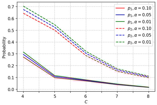
Figure 9.
Dependence of P on .
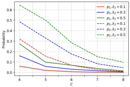
Figure 10.
Dependence of P on .
Table 4.
Values of joining probability .
Table 5.
Values of joining probability .
Table 6.
Values of joining probability .
Table 7.
Values of joining probability .
5. Conclusions
In this paper, the resource multi-server retrial queue with different rates of the service laws for different types of arrival customers and with breakdowns of servers modeling by the negative arrival process is analyzed. The capacity of the system resources is limited. The stationary distribution of the number of customers in the orbits and in the service unit is obtained under the asymptotic condition of the long delay in orbits. The comparison of the asymptotic results with simulation ones shows the high accuracy of our approach. Finally, we provide numerical examples to show the impact of the model parameters on some performance characteristics. Such analysis for the queuing system with a limited total amount of resources can be used in the process of communication network node design.
In the future, we plan to study multi-server resource retrial queuing systems with non-Poisson arrival processes and random values of the required resource. In addition, study of queuing systems with the service time depending on the required resource seems interesting.
Author Contributions
Conceptualization, E.L., E.F. and S.M.; methodology, E.L., R.S., E.F. and S.M.; software, E.L., R.S.; writing, original draft preparation, E.F.; writing, review and editing, E.L., R.S., E.F. and S.M.; supervision S.M. All authors have read and agreed to the published version of the manuscript.
Funding
This research received no external funding.
Institutional Review Board Statement
Not applicable.
Informed Consent Statement
Not applicable.
Data Availability Statement
Not applicable.
Conflicts of Interest
The authors declare no conflict of interest.
References
- Dudin, A.N.; Klimenok, V.I.; Vishnevsky, V.M. The Theory of Queuing Systems with Correlated Flows; Springer: Berlin/Heidelberg, Germany, 2020; 410p. [Google Scholar]
- Lakatos, L.; Szeidl, L.; Miklos, T. Introduction to Queueing Systems with Telecommunication Applications; Springer: Boston, MA, USA, 2013; 388p. [Google Scholar]
- Bocharov, P.; D’Apice, C.; Pechinkin, A.; Salerno, S. Queueing Theory; VSP: Utrecht, The Netherlands; Boston, MA, USA, 2004; 446p. [Google Scholar]
- Artalejo, J.R.; Gomez-Corral, A. Retrial Queueing Systems: A Computational Approach; Springer: Berlin/Heidelberg, Germany, 2008; 318p. [Google Scholar]
- Falin, G.I.; Templeton, J.G.C. Retrial Queues; Chapman and Hall: London, UK, 1997; 328p. [Google Scholar]
- Gelenbe, E. Product form networks with negative and positive customers. J. Appl. Prob. 1991, 28, 656–663. [Google Scholar] [CrossRef]
- Gelenbe, E. Harrison, P.; Pitel, E. The M/G/1 queue with negative customers. Adv. Appl. Probab. 1996, 28, 540–566. [Google Scholar]
- Bocharov, P.P.; Vishnevskii, V.M. G-Networks: Development of the theory of multiplicative networks. Automat. Rem. Control 2003, 64, 46–74. [Google Scholar]
- Chao, X.; Xiu, L.; Masakiyo, M.; Michael, P. Queueing Networks: Customers, Signals and Product Form Solutions; Wiley: Hoboken, NJ, USA, 1999; 464p. [Google Scholar]
- Matalytsky, M.; Zajac, P. Application of HM-network with positive and negative claims for finding of memory volumes in information systems. Appl. Math. Comput. Mech. 2019, 18, 41–51. [Google Scholar] [CrossRef]
- Do, T.V. Bibliography on G-networks, negative customers and applications. Math. Comput. Model. 2011, 53, 205–212. [Google Scholar] [CrossRef]
- Anisimov, V.; Artalejo, J.R. Analysis of Markov multiserver retrial queues with negative arrivals. Queueing Syst. 2001, 39, 157–182. [Google Scholar] [CrossRef]
- Shin, Y.W. Multi-server retrial queue with negative customers and disasters. Queueing Syst. 2007, 55, 223–237. [Google Scholar] [CrossRef]
- Kirupa, K.; Chandrika, K. Unreliable Batch Arrival Retrial Queue with Negative Arrivals, Multi-Types Of Heterogeneous Service, Feedback and Randomized J Vacations. Int. J. Comput. Appl. 2015, 127, 38–42. [Google Scholar]
- Fedorova, E.A.; Nazarov, A.A.; Farkhadov, M.P. Asymptotic Analysis of the MMPP/M/1 Retrial Queue with Negative Calls under the Heavy Load Condition. Izv. Saratov Univ. Math. Mech. Inform. 2020, 20, 534–547. [Google Scholar] [CrossRef]
- Dudin, A.; Dudina, O.; Dudin, S.; Samouylov, K. Analysis of Single-Server Multi-Class Queue with Unreliable Service, Batch Correlated Arrivals, Customers Impatience, and Dynamical Change of Priorities. Mathematics 2021, 9, 1257. [Google Scholar] [CrossRef]
- Atencia, I.; Galán-García, J.L. Sojourn Times in a Queueing System with Breakdowns and General Retrial Times. Mathematics 2021, 9, 2882. [Google Scholar] [CrossRef]
- Melikov, A.; Aliyeva, S.; Sztrik, J. Retrial Queues with Unreliable Servers and Delayed Feedback. Mathematics 2021, 9, 2415. [Google Scholar] [CrossRef]
- Nazarov, A.; Phung-Duc, T.; Paul, S.; Lizyura, O.; Shulgina, K. Central Limit Theorem for an M/M/1/1 Retrial Queue with Unreliable Server and Two-Way Communication. In Information Technologies and Mathematical Modelling. Queueing Theory and Applications. ITMM 2020. Communications in Computer and Information Science; Springer: Berlin/Heidelberg, Germany, 2021; Volume 1391, pp. 120–130. [Google Scholar]
- Tikhonenko, O.; Ziółkowski, M. Queueing systems with non–homogeneous customers and infinite sectorized memory space. Commun. Comput. Inf. Sci. 2019, 1039, 316–329. [Google Scholar]
- Tikhonenko, O.; Ziółkowski, M. Queueing Systems with Random Volume Customers and their Performance Characteristics. JIOS 2021, 45, 21–38. [Google Scholar] [CrossRef]
- Naumov, V.; Samouylov, K. Resource System with Losses in a Random Environment. Mathematics 2021, 9, 2685. [Google Scholar] [CrossRef]
- Naumov, V.; Samuilov, K. Analysis of networks of the resource queuing systems. Autom. Remote. 2018, 79, 822–829. [Google Scholar] [CrossRef]
- Efrosinin, D. Stepanova, N. Sztrik, J. Algorithmic Analysis of Finite-Source Multi-Server Heterogeneous Queueing Systems. Mathematics 2021, 9, 2624. [Google Scholar] [CrossRef]
- Lisovskaya, E.; Pankratova, E.; Moiseeva, S.; Pagano, M. Analysis of a Resource-Based Queue with the Parallel Service and Renewal Arrivals, Lecture Notes in Computer Science. Distrib. Comput. Commun. Netw. 2020, 12563, 335–349. [Google Scholar]
- Bushkova, T.; Moiseeva, S.; Moiseev, A.; Sztrik, J.; Lisovskaya, E.; Pankratova, E. Using Infinite-server Resource Queue with Splitting of Requests for Modeling Two-channel Data Transmission. Methodol. Comput. Appl. Probab. 2021, 1–20. [Google Scholar] [CrossRef]
- Bushkova, T.; Galileyskaya, A.; Lisovskaya, E.; Pankratova, E.; Moiseeva, S. Multi-service resource queue with the multy-component Poisson arrivals. Glob. Stoch. Anal. 2021, 8, 97–109. [Google Scholar]
- Moskaleva, F.; Lisovskaya, E.; Gaidamaka, Y. Resource Queueing System for Analysis of Network Slicing Performance with QoS-Based Isolation. In Information Technologies and Mathematical Modelling. Queueing Theory and Applications. ITMM 2020. Communications in Computer and Information Science; Springer: Berlin/Heidelberg, Germany, 2021; Volume 1391, pp. 198–211. [Google Scholar]
- Nazarov, A.; Moiseev, A.; Phung-Duc, T.; Paul, S. Diffusion Limit of Multi-Server Retrial Queue with Setup Time. Mathematics 2020, 8, 2232. [Google Scholar] [CrossRef]
- Dudin, S.; Dudin, A.; Dudina, O.; Samouylov, K. Analysis of a Retrial Queue with Limited Processor Sharing Operating in the Random Environment. In Wired/Wireless Internet Communications. WWIC 2017. Lecture Notes in Computer Science; Springer: Berlin/Heidelberg, Germany, 2017; Volume 10372, pp. 38–49. [Google Scholar]


Publisher’s Note: MDPI stays neutral with regard to jurisdictional claims in published maps and institutional affiliations. |
© 2022 by the authors. Licensee MDPI, Basel, Switzerland. This article is an open access article distributed under the terms and conditions of the Creative Commons Attribution (CC BY) license (https://creativecommons.org/licenses/by/4.0/).