CellsDeepNet: A Novel Deep Learning-Based Web Application for the Automated Morphometric Analysis of Corneal Endothelial Cells

Abstract

The quantification of corneal endothelial cell (CEC) morphology using manual and semi-automatic software enables an objective assessment of corneal endothelial pathology. However, the procedure is tedious, subjective, and not widely applied in clinical practice. We have developed the CellsDeepNet system to automatically segment and analyse the CEC morphology. The CellsDeepNet system uses Contrast-Limited Adaptive Histogram Equalization (CLAHE) to improve the contrast of the CEC images and reduce the effects of non-uniform image illumination, 2D Double-Density Dual-Tree Complex Wavelet Transform (2DDD-TCWT) to reduce noise, Butterworth Bandpass filter to enhance the CEC edges, and moving average filter to adjust for brightness level. An improved version of U-Net was used to detect the boundaries of the CECs, regardless of the CEC size. CEC morphology was measured as mean cell density (MCD, cell/mm²), mean cell area (MCA, μm²), mean cell perimeter (MCP, μm), polymegathism (coefficient of CEC size variation), and pleomorphism (percentage of hexagonality coefficient). The CellsDeepNet system correlated highly significantly with the manual estimations for MCD (r = 0.94), MCA (r = 0.99), MCP (r = 0.99), polymegathism (r = 0.92), and pleomorphism (r = 0.86), with p < 0.0001 for all the extracted clinical features. The Bland–Altman plots showed excellent agreement. The percentage difference between the manual and automated estimations was superior for the CellsDeepNet system compared to the CEAS system and other state-of-the-art CEC segmentation systems on three large and challenging corneal endothelium image datasets captured using two different ophthalmic devices.

1. Introduction

In Vivo Confocal Microscopy (IVCM) is a rapid non-invasive imaging method used to capture high-resolution images from all corneal layers [1]. The images acquired are useful to extract important clinical information and quantify morphological alterations in the human cornea to provide insights into a wide range of corneal endothelial cells’ pathologies and infections. The corneal endothelium is a monolayer of hexagonal corneal endothelial cells (CECs) that line the posterior surface of the cornea [2]. These CECs are vital for corneal transparency by maintaining an optimal state of corneal stromal hydration [3,4,5]. The corneal endothelial layer is comprised of 2300 to 2500 (cells/mm²), which are fixed-sized with uniform hexagonal forms and a honeycomb appearance [6]. The density, size, and shape of the CEC can be affected by ageing and a range of ocular and systemic pathologies as well as intraocular surgery [2]. CEC density and morphology can be used to define the functional ability of donor cornea before corneal transplantation [7,8].

Ideally, several morphological features define the health status of the corneal endothelium, including the Mean Cell Density (MCD) (cell/mm²), Mean Cell Area (MCA) (μm²), Mean Cell Perimeter (MCP), polymegathism, and pleomorphism. However, it has not been previously possible to accurately quantify these features [9]. Ophthalmologists and researchers have relied on the manual annotation to quantify endothelial cell density alone, which is very time-consuming and highly subjective [10]. It has also relied on assessing a particular Region of Interest (ROI) containing 20–30 cells and extrapolating to the whole cornea [7]. Therefore, the availability of an automatic image analysis system for accurate detection of the CEC boundaries and rapid geometric analysis of CEC morphology is essential to enable CEC pathology assessment in clinical settings [11]. Given the increasing clinical burden of diseases of the corneal endothelium, there is a need for rapid automated CEC quantification.

Designing and implementing a segmentation system for CECs has proven difficult due to poor image quality of the corneal endothelium [12]. Most of the early approaches applied simple methods (e.g., thresholding, Gaussian filtering, shape-dependent filters, and morphological operations) [13,14,15,16]. However, these approaches were limited due to the low contrast and uneven lighting of the input images, and relatively good results could only be obtained using high-quality images. Ruggeri et al. [7] proposed an automated estimation algorithm by applying a 2D-Discrete Fourier Transform (2D-DFT) for extracting the spatial frequencies embedded in 100 corneal endothelium images captured by an Inverse Phase Contrast Microscope (IPCM). The overall difference between the manual and automatic analysis of the endothelial cell density (ECD) was 14 (cells/mm²) with an execution time of 1 to 2 s per image. In 2015, Scarpa and Ruggeri [17] developed a CEC segmentation procedure using a genetic algorithm that they tested on a small database of 15 images acquired using specular microscopy and demonstrated a mean difference in ECD between manual and automated estimations of 4% with a maximum difference of less than 7%. Sharif et al. [18] developed a new model for detecting the CEC boundaries depending on Snake and Particle Swarm Optimization (S-PSO) by initially applying an image enhancement algorithm using 2D-DFT and Bandpass filter to improve the quality and decrease the noise presented in 11 corneal endothelium images and showed a mean difference between the manual and automated ECD of 5%. The automatic segmentation of CEC boundaries using the watershed approach and its variants is an applied solution. A market-driven watershed segmentation algorithm by Vincent and Masters [19] applied the watershed algorithm on the distance map [20] generated from the input image to generate a seeded stochastic watershed algorithm was developed by Selig et al. [21]. A slightly different algorithm was presented by Al-Fahdawi et al. [2] using a combination of the watershed algorithm and the Voronoi tessellations approaches to precisely trace the endothelial cell boundaries. However, the watershed approach and its variants are still prone to either under- or over-segmentation, especially in poor-quality images containing large endothelial cells.

Recently, several machine learning and deep learning approaches have been employed for the precise segmentation of corneal endothelial cell boundaries. Fabijanska [12] developed an effective endothelium cell segmentation system using a Feed-Forward Neural Network (F-FNN), trained to classify the image pixels into two classes (e.g., cell body or cell boundary). Nurzynska [22] proposed to train the Convolutional Neural Network (CNN) to precisely distinguish between three different regions: cell body, cell boundary, and cell centre. The performance of this approach was assessed on the “Alizarine” dataset [23], and a precision of 93%, a DICE of 0.94, and a Hausdorff distance of 0.14 pixel distance were achieved. Fabijanska [24] employed the U-Net on a dataset of 30 CEC images captured using specular microscopy to produce an edge probability map that was binarized and skeletonized to produce one-pixel wide borders. Relatively good results were obtained with a DICE of 0.85, AUROC of 0.92, and difference errors in ECD, CV, and HEC of 5.2%, 11.9%, and 6.2%, respectively. However, most of the existing approaches require user intervention to manually remove the incorrect borders or connect the discontinuous ones. Furthermore, a major limitation of most of the existing works is the use of small datasets, which cannot reveal how the trained network generalizes to a larger dataset of real-world CEC images unseen in the training set. Finally, a key concern of deep learning segmentation methods (e.g., CNN) is the extensive time needed to train a model to precisely trace the endothelial cell boundaries.

Segmentation systems can be utilized via a desktop or web application. Generally, desktop applications have limitations, especially for use in the clinic in relation to hardware requirements, the need for a specific operating system, and regular individual updates. Alternatively, web applications are more flexible and suitable for image segmentation systems, as the image processing and output are implemented on the server-side, and all users can easily access the web application. This paper provides a novel web application for the fully automated segmentation of CECs using a deep learning approach based on an improved version of U-Net architecture that correctly and accurately distinguishes cell boundaries and achieves precise segmentation. The main contributions of the current work are summarized below:

i.

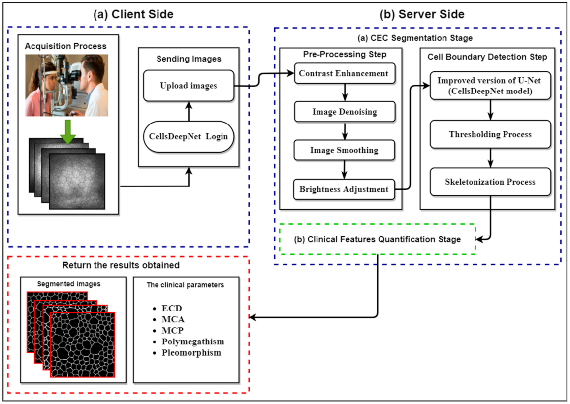
Development of CellsDeepNet, a novel, fully automated, and real-time web application for objective quantification of CEC morphology for CEC pathology assessment.

ii.

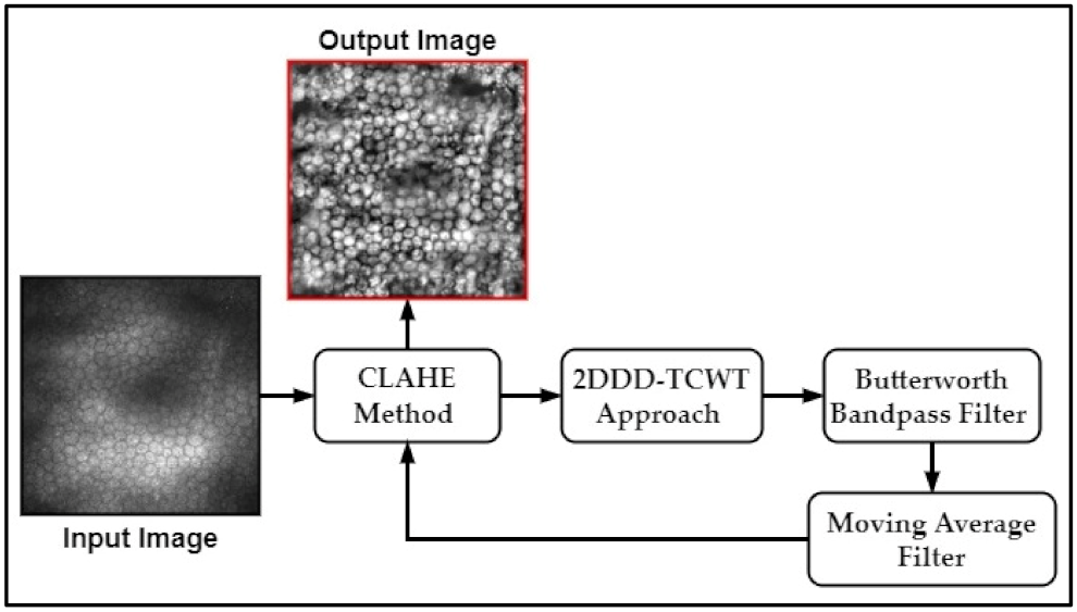
A new pre-processing procedure for reducing the noise and enhancing image quality is proposed to make cell boundaries more visible. Firstly, the contrast of the corneal endothelium image is improved by transforming the values using CLAHE. Secondly, novel image denoising and smoothing algorithms are proposed based on 2DDD-TCWT and Butterworth Bandpass filter to minimize the noise and enhance the edges of the corneal endothelial cell boundaries. This is followed by applying the brightness level adjustment step using the moving average filter and the CLAHE to reduce the effects of non-uniform illumination.

iii.

An improved version of U-Net architecture was applied to precisely identify all CEC boundaries in the enhanced image regardless of the endothelial cell size. An effective training methodology supported with some well-appointed training techniques (e.g., data augmentation, dropout technique, etc.) is utilized to assess different U-Net structures (e.g., the number of layers, the number of filters per layer, etc.) to prevent the overfitting issues and enhance the generalization capability of the final trained model.

iv.

The performance and generalization capability of the proposed CellsDeepNet system was verified in corneal endothelium images captured using corneal confocal microscopy (CCM) by the Heidelberg Retina Tomograph 3 with the Rostock Cornea Module (HRT 3 RCM) and a specular microscope. The results demonstrated that the measurement of the CEC morphology by the CellsDeepNet system highly correlates to the manual annotation and outperforms current state-of-the-art automated approaches on precise endothelial cell segmentation.

The remainder of this paper is structured as follows: Section 2 includes descriptions of the proposed CellsDeepNet system. The experimental results are presented in Section 3. Section 4 presents the conclusions and future research directions.

2. The Proposed CellsDeepNet System

The CellsDeepNet system is an entirely automatic system that needs no user interaction to precisely identify the CEC boundaries. As demonstrated in Figure 1, the CellsDeepNet system is comprised of the client-side and server-side. On the client-side, images of human CECs are acquired using CCM from patients. Then, the user/ophthalmologist goes to the CellsDeepNet login page to log in with their account. The CellsDeepNet web application allows the ophthalmologist to create a unique record for each patient that can be edited, viewed, and removed at any time. Once the patient’s record is created, all images are uploaded and sent to the server-side, where the core CellsDeepNet system produces the final segmented images and extracts useful endothelial cell parameters. On the server side, the proposed CellsDeepNet system comprises two stages: (a) CEC segmentation stage and (b) Clinical features quantification stage. The CEC segmentation stage is composed of (i) a ore-processing step to improve the CEC image quality and decrease the noise level and (ii) a cell boundaries detection step to precisely identify the CEC borders. In the clinical features quantification stage, a set of valuable clinical features are extracted as described previously [2].

2.1. Pre-Processing Step

The reliable calculation of the CEC parameters needs an accurate detection of the CEC boundaries in a large number of cells. However, CCM images suffer from various artefacts including blurriness, noise, non-uniform illumination, and low contrast (Figure 2) caused by: (i) saccadic eye movement causing a motion, blurring, or displacement effect; (ii) the spherical form of the cornea layer that can result in a non-uniform light distribution in various regions with darker areas in the periphery making the borders of cells unclear; and (iii) variation in the pressure level applied between the surface of the cornea and the CCM Tomocap.

In this study, an effective and reliable pre-processing procedure is developed to address the problems mentioned above, as shown in Figure 3. The main steps of the proposed image preprocessing procedure can be summarized as follows:

Step 1 (Contrast Enhancement): an adaptive contrast enhancement method is applied using the CLAHE method to improve the contrast of the CEC image [25]. The CLAHE method is based on Adaptive Histogram Equalization (AHE) that works on enhancing the contrast in small data regions, called tiles rather than the whole image, and neighboring tiles are fused using bilinear interpolation to reduce artificially induced borders. Herein, an optimized bilinear interpolation function is employed as in [26]. The main steps of the applied the CLAHE method can be outlined as follows:

(1)

Divide the input image of size (M × M) pixels into non-overlapping tiles of size (8 × 8) pixels.

(2)

Estimate the histogram of each tile in the input image.

(3)

Compute the clipping threshold value to redistribute pixels of each tile.

(4)

The histogram equalization is estimated for each tile of redistributed pixels.

(5)

The center pixel is computed of each tile, and then all pixels within a tile are produced using an optimized bilinear interpolation function to eliminate boundary artefacts.

In this work, the optimal value of the clip limit is set to 0.9. The contrast in the homogeneous regions can be restricted to avoid the over-enhancement of noise and decrease the edge-shadowing influence in the output image, as shown in Figure 4b.

Step 2 (Image Denoising): the 2DDD-TCWT approach is applied as a powerful image denoising technique to reduce noise and avoid destroying fine details (e.g., edges and curves) in the enhanced endothelial cell image, as displayed in Figure 4c. For the TCWT based denoising, we employed the ‘db4’ family wavelets. Many image denoising algorithms based on the wavelet framework have been proposed, but they suffer from weaknesses such as a lack of directionality, shift variance, oscillations, and aliasing [27]. In this work, to overcome these drawbacks, an efficient and robust image denoising approach using the 2DDD-TCWT and shrinkage operation is proposed to reduce the noise and recover the fine details in the endothelial cell image. In the wavelet domain, the coefficients having large absolute values correspond to the important information in the image, while commonly noise and very fine feature representations of the image are encoded by the coefficients having small absolute values. Hence, eliminating the coefficients with small absolute values and then rebuilding the image will produce an image with a lesser amount of noise. As described in [28], the major steps of image denoising based on the wavelet coefficients shrinkage approach can be summarized as follows:

(1)

The forward 2DDD-TCWT is applied to the input CEC image to determine the wavelet sub-bands coefficients.

(2)

The level of the noise variance in the input image is evaluated.

(3)

The non-linear shrinkage function is applied to compute the threshold value.

(4)

The soft thresholding technique is adopted based of the thresholding value computed in step 3.

(5)

Finally, the denoised image is obtained by applying the inverse 2DDD-TCWT.

In this work, the soft thresholding function $\left(\mathrm{T}=11\right)$ is applied in step 3, as described in [29].

Step 3 (Image Smoothing): the denoised image is then smoothed using the Butterworth Bandpass filter to reduce enhance the edges and curves in the endothelial cell image, as shown in Figure 4d. The Butterworth Bandpass filter is computed mathematically by multiplying the transfer functions of a low and high pass filter where the low pass filter has the higher cut-off frequency [30].

$$H_{LP} \left(u,v\right)=\frac{\mathbf{1}}{\mathbf{1}+{\left[D\left(u,v\right)/D_L\right]}^{\mathbf{2}n}}$$

(1)

$$H_{HP} \left(u,v\right)=\mathbf{1}-\frac{\mathbf{1}}{\mathbf{1}+{\left[D\left(u,v\right)/D_H\right]}^{\mathbf{2}n}}$$

(2)

$$H_{BP} \left(u,v\right)=H_{LP} \left(u,v\right)\times H_{HP} \left(u,v\right)$$

(3)

where $D_L$ and $D_H$ are the cut frequencies of the low and high pass filters and set to be 22 and 40, respectively; $n=\mathbf{3}$ is the filter order, and is $D\left(u,v\right)$ the distance from the origin.

Step 4 (Brightness Adjustment): the brightness level adjustment step using the moving average filter, and the CLAHE method is applied as described in step 1 (Contrast Enahancement) to reduce the effects of the non-uniform illumination of the image resulting from the previous step, as shown in Figure 4e. In this study, the moving average filter replaces each pixel with a weighted average of pixel values in a square of size (5 × 5) pixels centred at that pixel instead of forming a simple average. Let $f_{i.j}$, for $i,j=\mathbf{1},\mathbf{2},\dots ,n$, indicate the pixel values in the image and $g_{i.j}$ denote the output image. A linear filter of size $\left(\mathbf{2}m+\mathbf{1}\right)\times \left(\mathbf{2}m+\mathbf{1}\right)$, with identified weights $W_{k,l}$, for $k,l=-m,\dots ,m$, can be computed as follows:

$$g_{i.j}={\displaystyle \sum }_{k=-m}^m{\displaystyle \sum }_{l=-m}^m{W}_{k,l}\times f_{i+k.j+l}, for i, j=\left(m+\mathbf{1}\right),\dots ,\left(n-m\right)$$

(4)

2.2. Endothelial Cell Boundary Detection Step

Once the enhanced image is obtained, an effective segmentation algorithm using an improved version of the U-Net is applied to classify the pixels of the input image accurately and automatically into either the endothelial cell body or cell boundary. In the next sub-sections, the network architecture of the improved version of U-Net along with the followed training methodology are explained in detail.

2.2.1. Network Architecture

Many perspectives concerning the U-Net architecture along with the possible output generalization were investigated. The U-Net is mainly based on CNN, which was established to be used for biomedical image segmentation tasks. The main structure of the standard U-Net is composed of two main paths: a contracting path (called encoder) and an expanding path (called decoder). The encoder is a typical CNN and consists of the iterative application of convolutional layers, each followed by a rectified linear unit (ReLU) function and a max-pooling procedure. Through this contracting path, the size of the spatial data is reduced while more discriminative features are produced. On the other hand, the decoder integrates features and spatial data through a sequence of up-convolutional layers and concatenations with high-resolution and discriminative features obtained from the encoder path. Thus, the U-Net can efficiently produce the pixel-wise probability map of an image instead of classifying it as a whole. Compared to a typical CNN, the main structure of the U-Net was designed to work with fewer training images and to yield more precise segmentation.

The architecture of the proposed U-Net employed for detecting the boundaries of the CECs is depicted in Figure 5. It was derived from the original U-Net described in [31]. Unlike the original U-Net architecture, a set of modifications and enhancements were applied to produce precise endothelial cell segmentation. Firstly, the depth of the original U-Net was reduced by eliminating one layer from each path (e.g., contracting and expanding path) with the corresponding convolutions operations. Secondly, the filter size was changed to be (5 × 5) pixels instead of (3 × 3) pixels with a zero-padding of 2 pixels implemented at each layer to avoid a quick decrease in the amount of spatial data though moving toward the deepest layers. Thirdly, the number of trainable filters (feature maps) were changed to minimize the complexity of the last trained model and prevent the overfitting issues. Therefore, the number of trainable filters varies from 32 filters in the input layer to 128 filters in the deepest resolution layer. Finally, the dropout method as a regularization technique newly proposed by Srivastava et al. [32] was applied in between each two consecutive convolutional layers in the same level to avoid overfitting the training set and decreasing the complex co-adaptations of neurons by avoiding the inter-dependencies between them. In this work, the dropout is applied in each iteration of the training process by totally neglecting neurons with a probability of 0.5. At each path of the proposed network architecture, there are eight repeated applications of (5 × 5) convolutional filters, each followed by implementing a ReLU function.

The convolutional layers in the odd sequence are followed by applying the dropout method with a 0.5 parameter value to prevent the overfitting problem and learn more discriminative features. Furthermore, in the contacting path, a (2 × 2) max-pooling process with a stride of 2 pixels is implemented for down-sampling after each convolutional layer in the even sequence, in which the number of trainable filters was doubled. The main structure of the layers in the decoder path is identical to that in the encoder path, except that the max-pooling procedures were replaced with up-sampling procedures of the feature maps by a factor of 2. At decoder path, the total number of trainable filters was also halved, and the generated feature representations were merged with the analogous feature representations from the encoder path. A loss function based on cross-entropy along with Softmax activation was employed over the last convolutional layer in the decoder path to produce the probability distribution of two classes (e.g., cell body and cell boundary). Specifically, the loss function (https://en.wikipedia.org/wiki/Cross_entropy) (accessed on 10 December 2021) was defined as follows:

$$C\left(l,s\right)=w_{l_i}{\displaystyle \sum }_{i=0}^B{l}_i\log (s_i)+\left(\mathbf{1}-l_i\right)\log \left(\mathbf{1}-s_i\right)$$

(5)

where $s$ is the assigned pixel score, $l$ the reference pixel label, $B$ the total number of samples in one batch, and $w_{l_i}$ the pixel weight. The coss entropy is one of the most commonly used loss functions to measure how good DNNs perform. The value of the loss is computed as a numeric value between 0 and 1, with 0 being an optimal model. Thus, the main aim is to obtain a DNN model with a loss value as close to 0 as possible. To obtain the final segmented image, the edge probability map produced by the CellsDeepNet model was binarized and skeletonized to generate the one-pixel wide borders of the endothelial cells. In this step, the Hysteresis thresholding method was utilized to generate the binary image from the obtained edge probability map [33]. Using the Hysteresis thresholding method, all pixels with intensity value above the upper threshold $\left(T_{up}\right)$ are defined as cell boundary pixels. Furthermore, all the nearby pixels to these boundary pixels with intensity values higher than a lower threshold $\left(T_{low}\right)$ are defined as the cell’s boundary pixels as well. Herein, 8-connectivity was employed to detect the connected areas to each boundary point. Finally, the skeletonized image (e.g., one-pixel wide borders) was obtained by iteratively applying a thinning operation using the binary image produced from the Hysteresis thresholding method.

2.2.2. The Training Methodology

The corneal endothelium images and their corresponding manually segmented images (gold standard) were utilized to train the adopted model with the Stochastic Gradient Descent (SGD) technique for learning rate adaptability. Herein, all of the experiments were conducted by employing 60% randomly chosen images for the training set, while the remaining 40% was separated equally between the validation and testing sets. As described in [34], the suggested training methodology begins with training a specific network architecture using the training set and using the validation set to assess the generalization capability of the network through the learning process and store the weights of the model that performs best on it with a smallest validation error rate, as displayed in Figure 6. The proposed CellsDeepNet model was trained for 100 epochs with an initial learning rate of 0.01, a high momentum value (0.99), a weight decay parameter value (0.0005), and a mini-batch size of 100. In this study, the early stopping procedure was adopted during the learning process to determine the number of epochs where the learning process is stopped directly when the validation accuracy rate starts to decline due to the model starting to overfit the training data. On the other hand, the values of the most commonly used hyper-parameters (e.g., learning rate, mini-batch size, etc.) in the literature were employed. The major steps of the suggested training methodology can be outlined as follows:

(1)

Divide the dataset into 3 different sets: training set, validation set, and test set.

(2)

Choose an initial network architecture and a combination of training parameters.

(3)

Train the selected network architecture in step 2 using the training set.

(4)

Use the validation set to assess the performance of the selected network architecture through the training progression.

(5)

Repeat steps 3 through 4 by employing N = 100 epochs.

(6)

Choose the best-trained model with the smallest validation error.

(7)

Report the performance of the best model using the testing set.

In this work, the training and prediction procedures were implemented in the image-to-image sitting instead of the image-to-patch sitting employed in the original U-Net to reduce the system complexity, increase its throughput, and reduce the data redundancy due to overlapping patches. Figure 7 displays the loss and accuracy plots during the training process on the training and validation set of the MCCM and ECA dataset.

The data augmentation procedure is fundamental for the learning process associated with deep learning networks to prevent overfitting issues and enhance the generalization capability of the DNN. Given the nature of the corneal endothelium images, only eight random image patches of the same size were cropped from each corneal endothelium image and set to the size of the original image. Besides, the horizontal and vertical flipped versions were also obtained. Thus, ten images were generated from each corneal endothelium image. Figure 8 shows the ten image patches produced from a single CEC image using the employed data augementation procedure. In this work, other elastic deformations and transformations (e.g., rotation) were avoided for two reasons. Firstly, applying image rotation can produce new noise types, which do not exist in the CEC images. Secondly, the rotation process leads to losing the corners of the CEC image, which require to be filled either by reflecting the image or coloured the missing regions in black.

2.3. Clinical Features Quantification Stage

Five morphological measures are computed automatically from the final segmented CEC image, including mean cell density (MCD, cell/mm²), mean cell area (MCA, µm2), mean cell perimeter (MCP, µm), polymegathism, and pleomorphism. Using our web application, all these computed morphological measures can be reported in a PDF file that also contains coloured figures, patients’ information, and a table listing all the extracted features and a histogram distribution of the cell pleomorphism. The ophthalmologist can crop the selected ROI from the segmented CEC image, and the following morphological measures are computed as in [2].

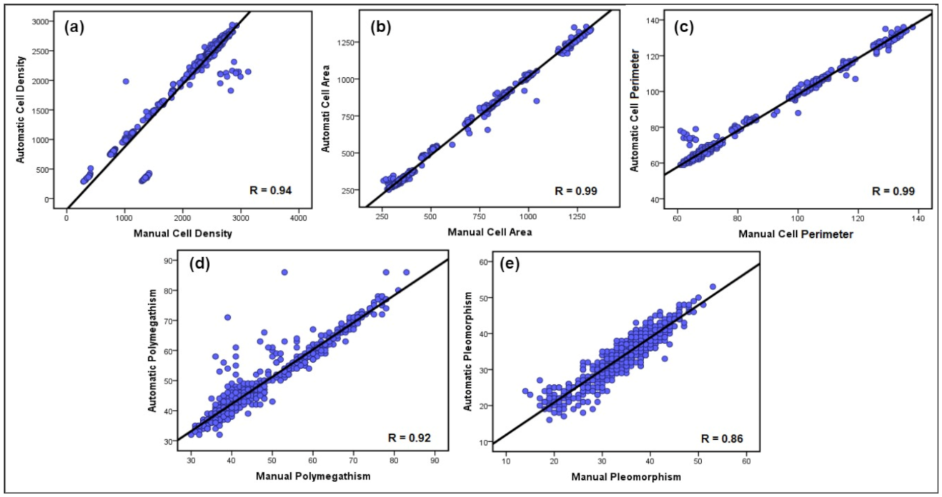
• MCD is computed by dividing the number of CECs $({\mathbf{C}}_{\mathbf{number}})$ in the selected ROI (otherwise entire segmented image) on the total size ${\left(\mathbf{S}\right)}_{ }$ of the selected ROI (otherwise entire segmented image) as follows:

  $$MCD=\frac{ C_{number}}{S_{ }}$$

  (6)
  Herein, to accurately estimate the MCD, only the cells on the two adjacent borders of the selected ROI are included, discarding them on other borders.
• Polymegathism also called Coefficient of Variation (CV), is utilized to define the difference in the endothelial cell’s area. Increasing the standard deviation ($STD$) value of the MCA can result in an imprecise estimate for the MCD. Therefore, increased polymegathism results in an imprecise estimation of MCA [6]. Polymegathism is computed as follows:

  $$Polymegathism=\frac{ST{D}_{cell area}}{MCA}\times 100$$

  (7)

  where $\mathbf{S}{\mathbf{D}}_{\mathbf{cell} \mathbf{area}}$ is the STD of the cell area divided by the MCA.
• Pleomorphism, also called Hexagonality Coefficient (HC), is computed by dividing the number of CECs with a roughly hexagonal form (neighbouring with 6 cells) C_hexagonal on the overall number of CECs in the selected ROI (otherwise entire segmented image) C_image as follows:

  $$Pleomorphism=\frac{C_{hexagonal}}{C_{image}}\times 100$$

  (8)

Some of the generated figures are displayed in Figure 9. Figure 9a shows a colour-coded map of the endothelial cells pleomorphism, where all CECs that neighbour the same number of cells are coded with the same colour. The CECs coloured orange correspond to six-sided cells. Figure 9b shows the histogram distribution plot of the pleomorphism parameter.

3. Experimental Results

In this work, several comprehensive experiments are carried out to measure the performance of the CellsDeepNet system in both detecting the endothelial cell boundaries and extracting useful clinical features. Firstly, the corneal endothelium image datasets employed in the conducted experiments are briefly described. This is followed by a comprehensive assessment and a comparison with the most current highly developed methods are presented. In this work, the partial correlation was employed to measure the strength of a relationship between the manual and automatic calculations of five clinical features. The cut-off of p-values was set to (p < 0.0001). Furthermore, the Bland–Altman plots were also used to confirm the agreement between manual and automatic endothelial cell parameters using the proposed CellsDeepNet system. A Bland–Altman plot comprises of a plot of the difference between paired evaluations of two parameters (e.g., the manual and automated estimations) over the average of these two estimations, with ±2 SD lines (agreements outlines) parallel to the mean difference line.

3.1. Datasets Description

The performance of the developed CellsDeepNet system was assessed using two different challenging datasets, termed the Manchester Corneal Confocal Microscopy (MCCM) dataset [35] and Endothelial Cell Alizarine (ECA) dataset [23].

• Manchester Corneal Confocal Microscopy Dataset: The MCCM dataset contains a total of 1010 images of CECs acquired using the Heidelberg Retinal Tomograph III Rostock Cornea Module (Heidelberg Engineering GmbH, Heidelberg, Germany). This device uses a 670 nm red wavelength diode laser, which is a class I laser and therefore does not pose any ocular safety hazard. A 63× objective lens with a numerical aperture of 0.9 and a working distance relative to the applanating cap (TomoCap, Heidelberg Engineering GmbH, Heidelberg, Germany) of 0.0 to 3.0 mm was used. The images produced using this lens are (400 μm × 400 μm) with a (15°×15°) field of view and 10 μm/pixel transverse optical resolution. The cornea was locally anaesthetized by instilling 1 drop of 0.4% benoxinate hydrochloride (Chauvin Pharmaceuticals, Chefaro, UK), and Viscotears (Carbomer 980, 0.2%, Novartis, UK) was used as the coupling agent between the cornea and the TomoCap as well as between the TomoCap and the objective lens. The patients were asked to place their chin on the chin rest and press their forehead against the forehead support. They were asked also to fixate with the eye not being examined on an outer fixation light to enable examination of the central cornea. Images of the endothelial cells were captured using the “section” mode. Multiple images were taken from the endothelium immediately posterior to the posterior stroma. On CCM, endothelial cells are identified as a polygonal shape with bright cell bodies and dark borders. During image acquisition, 2–3 representative sharp images were selected by filtering out blurred images, pressure lines, or dark shadows caused by the pressure applied between the TomoCap and cornea or out of focus images. Some samples of unprocessed corneal endothelium images are presented in Figure 2. It is worth noting that the corneal endothelium images used in this dataset are very challenging poor-quality images compared to those used in the previous works. A major challenge for carrying out this research using this dataset was the unavailability of ground-truth images and the reference value measurements for all five clinical parameters. To obtain a manual version from this database, a freely available application, named GNU Image Manipulation Program (GIMP) was utilized by an expert ophthalmologist from the University of Manchester to manually detect endothelial cell boundaries and then generate a binary image from particular ROIs to serve as a ground-truth image in the segmentation evaluation and a manual estimation of the reference values of the clinical parameters, as shown in Figure 10.
• Endothelial Cell Alizarine Dataset: This dataset is composed of 30 corneal endothelium images captured by an IPCM (CK 40, Chroma Technology Corp, Windham, VT, USA) at (200 × magnification) and an analogue camera (SSC-DC50AP, Sony, Tokyo, Japan) [23]. These images were taken from 30 porcine eyes stained with alizarine and stored in the JPEG format of resolution (576 × 768) pixels. The ground truth images representing the borders of the endothelial cells traced manually by an expert ophthalmologist are also provided. Each image contains approximately 232 detected cells on average (ranging from 188 to 388 cells), along with an average cell area of 272.76 pixels. This dataset is freely available at http://bioimlab.dei.unipd.it, accessed on 10 December 2021.

3.2. Experiments on MCCM Dataset

Using the MCCM dataset, several experiments were carried out to measure the performance of the CellsDeepNet system. Firstly, the performance of the CellsDeepNet system was validated against the gold standard images (e.g., binary images) produced from the GIMP software, as shown in Figure 10c. In this assessment procedure, seven quantitative performance measurements were computed, including: Probabilistic Rand Index (PRI) [36], Gradient Magnitude Similarity Deviation (GMSD) [37], Structural SIMilarity (SSIM) Index [38], Variation of Information (VoI) [39], Normalized Absolute Error (NAE), Mean Square Error (MSE) [40], and Global Consistency Error (GCE) [41]. These employed seven quantitative metrics are commonly used in the previous works for measuring the effectiveness and reliability of segmentation algorithms. In this work, the performance of the developed CellsDeepNet system was compared with our previous fully-automated Corneal Endothelium Analysis System (CEAS) described in [2] as well as with the original U-Net structure described in [31]. Initially, the impact of the image enhancement procedure was assessed by training the improved U-Net from scratch on top of enhanced CEC images instead of the direct usage of the raw CEC images to guide the learning process by enforcing the U-Net to learn only discriminating features. As shown in

Table 1. Performance comparison study of the proposed CellsDeepNet system with and without applying the image pre-processing step.

Quantitative Measures	MCCM Dataset		ECA Dataset
	With Image Pre-Processing	Without Image Pre-Processing	With Image Pre-Processing	Without Image Pre-Processing
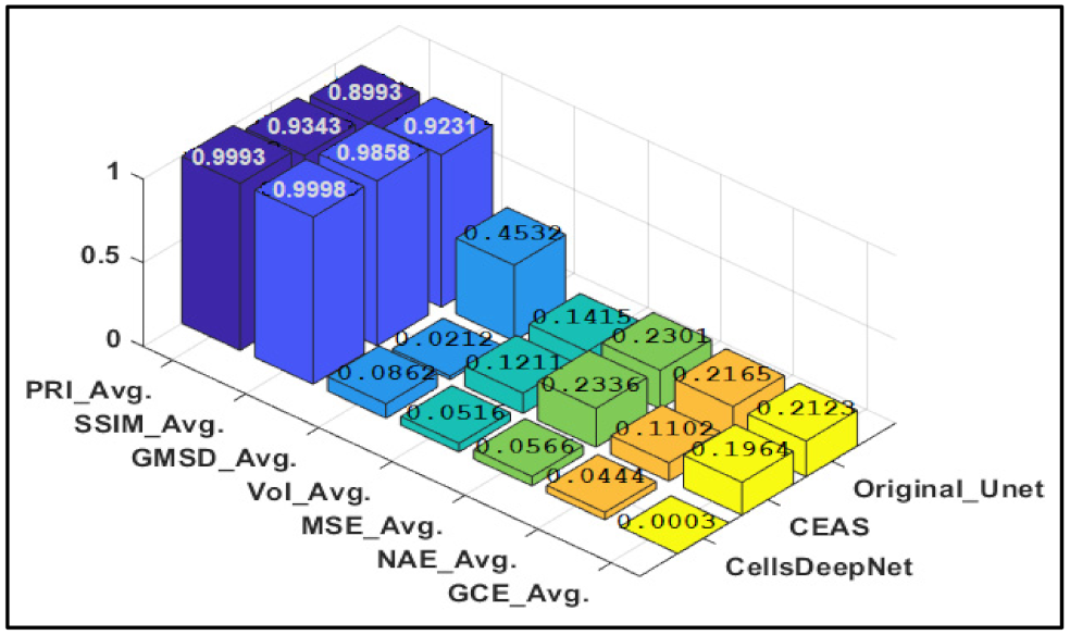
PRI	0.9993	0.4956	0.9837	0.5053
SSIM	0.9998	0.4102	0.9768	0.4312
VoI	0.0516	0.7231	0.1032	0.8901
GMSD	0.0862	0.8231	0.0105	0.9212
MSE	0.0566	0.5342	0.0337	0.5231
GCE	0.0003	0.5223	0.0006	0.4345
NAE	0.0444	0.4532	0.0769	0.5301

, we demonstrate that the developed CellsDeepNet system can accurately identify the boundaries of the CECs regardless of endothelial cell size.

The total average of the employed seven quantitative metrics was significantly increased in comparison with the direct usage of the raw CEC images. Moreover, the time required to obtain the final trained model was about 20 min compared to approximately one hour and 45 min using the raw CEC images. The overall average of these seven quantitative metrics was calculated for all the CCM images in the MCCM dataset and compared in Figure 11. Of note, better results were obtained from both CellsDeepNet and CEAS systems compared to the original U-Net in terms of all seven quantitative measurements.

Although the CEAS system has got a superior result of GMSD measurement (0.0212) compared to 0.0862 produced from the proposed CellsDeepNet system, it produced lower results in terms of the other six quantitative measures. There were no substantial differences found between the automated segmented images using the developed CellsDeepNet system and the manual images. In the second experiment, the effectiveness and robustness of the CellsDeepNet system were assessed by comparing the automatic estimations of the five clinical parameters with reference values computed by applying the definition of these clinical features on the binary image produced from the GIMP software. Initially, the outputs using both the CellsDeepNet and CEAS system were obtained from all corneal endothelium images in the MCCM dataset. Then, the identical ROI with the biggest region of visible CECs was chosen for that image and used to automatically compute the values of the five clinical parameters. Next, the automatic estimations of the clinical parameters were compared with the reference values.

Table 2. Measures of the CEC morphology generated by manual assessment, CEAS, and CellsDeepNet system from the MCCM dataset. The differences (Diff) between the manual and automated estimates are listed along with a percentage (Diff %).

	Manual	Auto. CEAS System			Auto. CellsDeepNet System
	MCD (Cells/mm2)	MCD (Cells/mm2)	Diff	Diff %	MCD (Cells/mm2)	Diff	Diff %
Av.	1898.08	1967.04	31.04	1.56	1984.88	13.2	0.66
STD	765.21	755.55	9.66	1.27	763.17	2.04	0.26
Max	3125	3226	−101	−3.18	2937	188	6.20
Min	1232	1280	−48	−3.82	1230	2	0.16
	MCA (µm2)	MCA (µm2)	Diff	Diff %	MCA (µm2)	Diff	Diff %
Av.	292.28	285	7.28	2.52	292.27	0.01	0.003
STD	41.77	44.45	−2.68	−6.21	41.76	0.01	0.02
Max	395	390	5	1.27	395	0	0
Min	229	233	−4	−1.73	229	0	0
	MCP (µm)	MCP (µm)	Diff	Diff %	MCP (µm)	Diff	Diff %
Av.	79.04	74.06	4.98	6.50	77.16	1.88	2.40
STD	20.55	21.67	−1.12	−5.30	20.93	−0.38	−1.83
Max	138	140	−2	−1.43	136	2	1.45
Min	61	63	−2	−3.22	59	2	3.33
	Polymegathism %	Polymegathism %	Diff	Diff %	Polymegathism %	Diff	Diff %
Av.	45.44	42.95	2.49	5.6	44.14	1.3	2.90
STD	11.14	12.68	−1.54	−12.93	10.48	0.66	6.10
Max	83	79	4	4.93	86	−3	−3.55
Min	30	34	−4	−12.5	32	−2	−6.45
	Pleomorphism %	Pleomorphism %	Diff	Diff %	Pleomorphism %	Diff	Diff %
Av.	34.78	32.5	2.28	6.77	34.19	0.59	1.71
STD	6.14	3.63	2.51	51.38	5.98	0.16	2.64
Max	53	56	−3	−5.50	53	0	0
Min	14	17	−3	−19.35	16	−2	−13.33

shows the total average, STD, MAX, and MIN of each clinical feature for both manual and automatic segmented CEC images, in addition to the difference and the percentage difference between them. Although the CEAS system achieved good agreement with reference values, a higher agreement was achieved with the proposed CellsDeepNet system. The average percentage variations between manual and automated estimates computed using the CEAS and CellsDeepNet system were 1.56% vs. 0.66%, 2.52% vs. 0.003%, 6.5% vs. 2.4%, 5.6% vs. 2.9%, and 6.8% vs. 1.7% for MCD, MCA, MCP, polymegathism, and pleomorphism, respectively. There were highly significant correlations between the manual and automated estimates for MCD (r = 0.94), MCA (r = 0.99), MCP (r = 0.99), polymegathism (r = 0.92), and pleomorphism (r = 0.86), with p < 0.0001 for all the extracted clinical features, as shown in Figure 12. As shown in Figure 13, one can see that MCD is located between 966 to 2925 (cell/mm²), MCA is located between 266 to 1328 (μm²), MCP is located between 60 to 137 (μm), polymegathism is located between 31 to 85%, and pleomorphism is located between 18 to 53%.

3.3. Experiments on ECA Dataset

To prove the generalization capability of the developed CellsDeepNet system, seven quantitative performance measurements from both the automated segmented images and ground-truth images were applied to the ECA dataset. The performance comparison between three different segmentation systems (U-Net, CellsDeepNet, and CEAS system) on the ECA dataset was tested using seven quantitative metrics (Figure 14). Even though the performance of the original U-Net improved slightly on the ECA dataset, it was inferior to both the CellsDeepNet and CEAS systems. The results obtained by the CellsDeepNet system compared to the CEAS system were better for all seven quantitative measurements. The automated estimation of all five CEC parameters were compared to the reference values from the same ROI (

Table 3. Performance comparison between the manual and automatic estimates of five clinical parameters from the ECA dataset.

	Manual	Auto. CEAS System			Auto. CellsDeepNet System
	MCD (Cells/mm2)	MCD (Cells/mm2)	Diff	Diff %	MCD (Cells/mm2)	Diff	Diff %
Av.	2952	2925	27	0.91	2927	25	0.85
STD	161	157	4	2.51	158	3	1.88
Max	3194	3177	17	0.53	3181	13	0.40
Min	2662	2605	57	2.16	2612	50	1.89
	MCA (µm2)	MCA (µm2)	Diff	Diff %	MCA (µm2)	Diff	Diff %
Av.	274	269	5	1.84	272	2	0.73
STD	16.08	15.65	0.43	2.71	16.01	0.07	0.43
Max	305	300	5	1.65	306	−1	−0.32
Min	251	246	5	2.01	247	4	1.60
	MCP (µm)	MCP (µm)	Diff	Diff %	MCP (µm)	Diff	Diff %
Av.	66.68	65.58	1.1	1.66	65.20	1.48	2.24
STD	2.76	1.67	1.09	49.20	2.82	−0.06	−2.15
Max	92	90	2	2.19	87	5	5.58
Min	56	58	−2	−3.50	59	−3	−5.21
	Polymegathism %	Polymegathism %	Diff	Diff %	Polymegathism %	Diff	Diff %
Av.	31.81	30.54	1.27	4.07	31.65	0.16	0.50
STD	2.85	2.68	0.17	6.14	2.83	0.02	0.70
Max	38	42	−4	−10	38	0	0
Min	26	29	−3	−10.9	26	0	0
	Pleomorphism %	Pleomorphism %	Diff	Diff %	Pleomorphism %	Diff	Diff %
Av.	40.84	37.5	3.34	8.52	40.68	0.16	0.39
STD	1.73	2.52	−0.79	−37.17	1.95	−0.22	−11.95
Max	46	44	2	4.44	47	−1	−2.15
Min	36	33	3	8.69	36	0	0

). The average percentage differences between manual and automatic estimations calculated using the CEAS and CellsDeepNet system were 0.91% vs. 0.85%, 1.84% vs. 0.73%, 1.66% vs. 2.24%, 4.07% vs. 0.50%, and 8.52% vs. 0.39% for MCD, MCA, MCP, polymegathism, and pleomorphism, respectively. There were highly remarkable correlations between the manual and automated estimations for MCD (r = 0.98), MCA (r = 0.98), MCP (r = 0.86), polymegathism (r = 0.91), and pleomorphism (r = 0.76) with the cut-off of p-values set to (p < 0.0001), as shown in Figure 15.

The Bland–Altman plots confirm the excellent agreement between manual and automatic endothelial cell parameters using the CellsDeepNet system. As shown in Figure 16, one can see that the MCD is located between 2637 and 3185 (cell/mm²); MCA is located between 250 and 306 (μm²); MCP is located between 58 and 90 (μm); polymegathism is located between 27 and 38%; and pleomorphism is located between 36 and 46%.

Figure 17 shows the overlap segmented image of the manual and automated outputs to visually demonstrate the endothelial cell segmentation truthfulness of the proposed CellsDeepNet system. In this figure, the yellow lines refer to the ground-truth segmented image, and the purple lines refer to the automatic output of the CellsDeepNet system, whereas the white lines describe the common borders of the endothelial cells.

3.4. Comparison Study

In this section, the performance of the developed CellsDeepNet system was compared against six present state-of-the-art CEC segmentation systems using the EAC dataset, as illustrated in

Table 4. Performance comparison between the CellsDeepNet system and the existing CEC segmentation systems using three clinical parameters.

		Scarpa and Ruggeri [17]		Ruggeri et al. [23]		Poletti and Ruggeri [42]		CellsDeepNet System
MCD (cells/mm2)		Diff	Diff %	Diff	Diff %	Diff	Diff %	Diff	Diff %
	Av.	17.73	0.82	−12	0.28	96.35	3.11	25	0.85
	STD	16.31	1.08	−10	3.1	58.83	2.29	3	1.88
	Max	0	0	−7	0.18	18	0.57	13	0.40
	Min	3.80	6.24	35	0.72	245	10.37	50	1.89
Polymegathism %		Diff	Diff %	Diff	Diff %	Diff	Diff %	Diff	Diff %
	Av.	1.45	3.95	0.7	3.02	5.72	14.78	0.16	0.50
	STD	0.79	1.93	0.2	6.89	2.56	5.90	0.02	0.70
	Max	0	0	1.1	6.41	1.10	2.20	0	0
	Min	2.80	6.86	−0.1	0.35	12.20	24.30	0	0
		Diff	Diff %	Diff	Diff %	Diff	Diff %	Diff	Diff %
Pleomorphism %	Av.	1.83	3.13	−0.5	1.03	4.21	7.32	0.16	0.39
	STD	1.33	2.27	−0.9	23.37	2.72	4.57	−0.22	−11.95
	Max	0	0	2.2	5.62	0	0	−1	−2.15
	Min	3.80	6.24	−4.2	7.47	11.80	16.21	0	0

. The first system was established by Ruggeri et al. [23], in which the luminosity correction and contrast enhancement of the corneal endothelium image was enhanced using a parabolic correction and a sigmoid point transformation, respectively. The boundaries of the endothelial cells were detected by training a multi-layer F-FNN to classify each pixel in the input image either as a cell body or cell boundary. The second system proposed by Scarpa and Ruggeri [17] used a genetic algorithm combining information about the shape of the CECs and the intensity of the pixels to detect the endothelial cell boundaries. The third one developed by Poletti and Ruggeri [42] uses three different kernels specially designed to compute three endothelial cell signatures (e.g., vertex, side, or body). These extracted signatures were utilized as feature vectors to train a SVM classifier to correctly detect the boundaries of the CECs. In this comparison study, MCD, polymegathism, and pleomorphism were compared due to the limitation of these systems to compute the other CEC parameters. Compared to the method of Ruggeri et al. [23], the CellsDeepNet system achieved a slightly worse Diff % for MCD (0.28 v 0.85), but it was better for polymegathism (3.02% v 0.50%) and pleomorphism (1.03% v 0.39%). Compared to the Poletti and Ruggeri system [42], CellsDeepNet system achieved a slightly worse Diff % for MCD (0.82% v 0.85%), but it was better for polymegathism (3.95% v 0.50%) and pleomorphism (3.13% v 0.39%). Compared to the method of Scarpa and Ruggeri [17] the CellsDeepNet system achieved better outcomes for MCD (3.11% v 0.85%), but it was better for polymegathism (14.78% v 0.50%) and pleomorphism (7.32% v 0.39%).

The performance of the CellsDeepNet system was also compared with some of the state-of-the-art deep learning-based CEC segmentation systems (e.g., Fabija’nska [24], Zhang et al. [43], Nurzynska [22], and U-Net [31]) by the conduction of several comprehensive experiments using the same dataset. In these experiments, six measures were computed, such as Dice Coefficient (DI), Jaccard coefficient (JA), F1 Score (F1), Specificity (SP), Sensitivity (SE), and Modified Hausdorff Distance (MHD) as evaluation metrics. The first three measures are more related to reveal the overall level between the manual and automatic segmentation. As shown in

Table 5. Performance comparison between the proposed CellsDeepNet system with other existing deep learning CEC segmentation systems using the EAC dataset.

Models	Measures
	DI	JA	F1	SP	SE	MHD
Fabija´nska [24]	0.86	-	-	-	-	-
Zhang et al. [43],	0.78	-	0.82	0.94	0.87	-
Nurzynska [22]	0.94	0.94	-	-	-	0.14
Orig. U-Net [31]	0.77	0.79	0.81	0.96	0.81	0.22
CellsDeepNet	0.97	0.98	0.89	0.98	0.90	0.08

, the proposed CellsDeepNet system has achieved the best overall performance on the EAC dataset in term of the six adopted evaluation metrics. It is worth mentioning that the CEC segmentation system developed by Fabija’nska [24] achieved a proportional difference of 5.2% for MCD, 6.2% for pleomorphism, and 11.93% for polymegathism, while no clinical feature with a proportional difference (>2.5%) has been achieved using the proposed CellsDeepNet system.

Further experiments were carried out by testing the performance of the developed CellsDeepNet system on the dataset provided by Selig et al. [21]. This dataset composed of 52 CEC images acquired from 23 patients using in vivo confocal corneal microscopy. Using the automated cell segmentation results provided by Selig et al. [21], the seven adopted quantitative performance measurements were computed and compared with the proposed CellsDeepNet system, as shown in Figure 18. The results obtained by the proposed CellsDeepNet system compared to the Selig et al. [21] system were better for all seven quantitative measurements.

Figure 19 displays a comparison between the automatically segmented CEC images produced by the developed CellsDeepNet system and Selig et al. [21] system. It is clear that the Selig et al. [21] system suffers from the over-segmentation problem, especially in detecting the endothelial cells with large sizes. The incorrectly segmented endothelial cell boundaries are filled with the red colour.

3.5. Discussion

The study has shown a quantitatively better performance using the proposed CellsDeepNet system compared to U-Net and the SEAS system on two large and challenging corneal endothelium image datasets captured using two different devices. For instance, using the MCCM dataset, the mean difference between manual and automated estimates was lower than 1%, 0.05%, 2.5%, 3%, and 2% for MCD, MCA, MCP, polymegathism, and pleomorphism, respectively, with no clinical feature with a proportional difference (>3%) between the manual and automated estimates. The proposed CellsDeepNet system provides an accurate estimation for all the five clinical features of the detected CECs, with higher than (95%) of the information falling between ±2 SD lines, as shown in Figure 13. In this experiment, one can see that MCD is located between 966 and 2925 (cell/mm²); MCA is located between 266 and 1328 (μm²); MCP is located between 60 and 137 (μm); polymegathism is located between 31 and 85%; and pleomorphism is located between 18 and 53%.

Using the ECA dataset derived from a specular microscope, which is most commonly used in most ophthalmology clinics, the mean differences between manual and automated estimates were less than 1%, 1%, 2.5%, 0.5%, and 0.5% for MCD, MCA, MCP, polymegathism, and pleomorphism, respectively, with no clinical feature with a proportional difference (>2.5%) between the manual and automated estimates. Better results were obtained using all the employed systems on the ECA dataset, as the images were of higher quality compared to the images obtained for the MCCM dataset which used a CCM.

Furthermore, the developed CellsDeepNet system based on the modified U-Net architecture significantly reduced the time necessary to obtain the last trained model to 20 min compared with the original U-Net model, which takes approximately one hour and 45 min. The proposed CellsDeepNet web application has a number of advantages. It is more flexible and suitable for researchers or ophthalmologists, as they do not need specific hardware, given that the processing to produce the final segmented image and quantitative output is implemented on the server-side. In addition, clinicians can create a unique record for each patient that can be edited, viewed, and removed at any time. The selection of an ROI from the final segmented image allows for the inspection of the segmentation results to automatically extract more accurate and useful clinical parameters from the clearest ROI in the segmented image. The results obtained using the CellsDeepNet system are encouraging, especially as they have been obtained from two large image data sets of corneal endothelial cells from two different microscopes. However, there are some limitations, including over-segmentation, especially when poor quality images containing large CEC’s are fed into the CellsDeepNet system. The accuracy of the CellsDeepNet system may be enhanced by extending the training set using a larger and more heterogeneous dataset of corneal endothelial images.

4. Conclusions and Future Work

We have developed the CellsDeepNet system, an improved, fully automated, and fast corneal endothelial cell analysis system. It requires no user intervention for segmenting and extracting different corneal endothelial cell parameters. Two different datasets of corneal endothelium images acquired using a specular microscope and corneal confocal microscope along with their manually traced ground-truth images were employed to validate the performance of the developed CellsDeepNet system. An efficient and reliable pre-processing procedure was deployed to eliminate the noise, improve the image quality, and make the boundaries of CECs more visible, and an improved version of the U-Net architecture was used to produce a binary segmented image of the endothelial cell boundaries to enhance the quantification of clinically useful parameters. Our results demonstrate the effectiveness, reliability, and superior outcomes of the CellsDeepNet system compared to the current highly developed approaches in terms of segmentation precision and the extraction of clinically useful endothelial cell parameters. This markedly increases the clinical utility of this image analysis system, especially as it is web-based to allow rapid (<3 s/image) corneal endothelial cell quantification to identify pathology and assess disease progression over time. We are not presenting the final word in accurately detecting the endothelial cell boundaries and extracting useful clinical features. We are currently in the process of testing the accuracy of the proposed CellsDeepNet system using a larger and more challenging dataset, in which the corneal endothelium images are captured using different microscope devices.

References

- Al-Fahdawi, R.S.; Qahwaji, A.R.S.; Al-Waisy, S.; Ipsopn, S. An Automatic Corneal Subbasal Nerve Registration System Using FFT and Phase Correlation Techniques for an Accurate DPN Diagnosis. In Proceedings of the 2015 IEEE International Conference on Computer and Information Technology; Ubiquitous Computing and Communications; Dependable, Autonomic and Secure Computing; Pervasive Intelligence and Computing, Liverpool, UK, 26–28 October 2015; pp. 1035–1041. [Google Scholar] [CrossRef]
- Al-Fahdawi, S.; Qahwaji, R.; Al-Waisy, A.S.; Ipson, S.; Ferdousi, M.; Malik, R.A.; Brahma, A. A fully automated cell segmentation and morphometric parameter system for quantifying corneal endothelial cell morphology. Comput. Methods Programs Biomed. 2018, 160, 11–23. [Google Scholar] [CrossRef]
- Al-Fahdawi, S.; Qahwaji, R.; Al-Waisy, A.S.; Ipson, S.; Malik, R.A.; Brahma, A.; Chen, X. A fully automatic nerve segmentation and morphometric parameter quantification system for early diagnosis of diabetic neuropathy in corneal images. Comput. Methods Programs Biomed. 2016, 135, 151–166. [Google Scholar] [CrossRef] [Green Version]
- Gavet, Y.; Pinoli, J.-C. Comparison and Supervised Learning of Segmentation Methods Dedicated to Specular Microscope Images of Corneal Endothelium. Int. J. Biomed. Imaging 2014, 2014, 704791. [Google Scholar] [CrossRef] [PubMed]
- Khan, A.; Kamran, S.; Akhtar, N.; Ponirakis, G.; Al-Muhannadi, H.; Petropoulos, I.N.; Al-Fahdawi, S.; Qahwaji, R.; Sartaj, F.; Babu, B.; et al. Corneal Confocal Microscopy detects a Reduction in Corneal Endothelial Cells and Nerve Fibres in Patients with Acute Ischemic Stroke. Sci. Rep. 2018, 8, 17333. [Google Scholar] [CrossRef]
- McCarey, B.E.; Edelhauser, H.F.; Lynn, M.J. Review of Corneal Endothelial Specular Microscopy for FDA Clinical Trials of Refractive Procedures, Surgical Devices and New Intraocular Drugs and Solutions. Cornea 2008, 27, 1–16. [Google Scholar] [CrossRef] [Green Version]
- Ruggeri, A.; Grisan, E.; Jaroszewski, J. A new system for the automatic estimation of endothelial cell density in donor corneas. Br. J. Ophthalmol. 2005, 89, 306–311. [Google Scholar] [CrossRef] [Green Version]
- Gain, P.; Thuret, G.; Kodjikian, L.; Gavet, Y.; Turc, P.H.; Theillere, C.; Acquart, S.; Le Petit, J.C.; Maugery, J.; Campos, L. Automated tri-image analysis of stored corneal endothelium. Br. J. Ophthalmol. 2002, 86, 801–808. [Google Scholar] [CrossRef] [PubMed]
- Doughty, M.J.; Aakre, B.M. Further analysis of assessments of the coefficient of variation of corneal endothelial cell areas from specular microscopic images. Clin. Exp. Optom. 2008, 91, 438–446. [Google Scholar] [CrossRef] [PubMed]
- Foracchia, M.; Ruggeri, A.M. Cell contour detection in corneal endothelium in-vivo microscopy. In Proceedings of the 22nd Annual International Conference of the IEEE Engineering in Medicine and Biology Society, Chicago, IL, USA, 23–28 July 2000; Volume 2, pp. 1033–1035. [Google Scholar] [CrossRef]
- Foracchia, M.; Ruggeri, A.M. Corneal Endothelium Cell Field Analysis by means of Interacting Bayesian Shape Models. In Proceedings of the 2007 29th Annual International Conference of the IEEE Engineering in Medicine and Biology Society, Lyon, France, 22–26 August 2007; Volume 62035–60387, pp. 6035–6038. [Google Scholar] [CrossRef]
- Fabijańska, A. Corneal Endothelium Image Segmentation Using Feedforward Neural Network. In Proceedings of the Federated Conference on Computer Science and Information Systems, Prague, Czech Republic, 3–6 September 2017; Volume 11, pp. 629–637. [Google Scholar] [CrossRef] [Green Version]
- Nadachi, R.; Nunokawa, K. Automated Corneal Endothelial Cell Analysis. In Proceedings of the Fifth Annual IEEE Symposium on Computer-Based Medical Systems, Durham, NC, USA, 14–17 June 1992; pp. 450–457. [Google Scholar]
- Mahzoun, M.; Okazaki, K.; Mitsumoto, H.; Kawai, H.; Sato, Y.; Tamura, S.; Kani, K. Detection and Complement of Hexagonal Borders in Corneal Endothelial Cell lmage. Med. Imaging Technol. 1996, 14, 56–69. [Google Scholar]
- Sanchez-Marin, F.J. Automatic segmentation of contours of corneal cells. Comput. Biol. Med. 1999, 29, 243–258. [Google Scholar] [CrossRef]
- Ayala, G.M.E.D.H.; Mart, L.H. Granulometric moments and corneal endothelium status. Pattern Recognit. 2001, 34, 1219–1227. [Google Scholar] [CrossRef]
- Scarpa, F.; Ruggeri, A. Segmentation of Corneal Endothelial Cells Contour by Means of a Genetic Algorithm. In Proceedings of the Ophthalmic Medical Image Analysis Second International Workshop, OMIA 2015, Held in Conjunction with MICCAI 2015, Munich, Germany, 9 October 2015; pp. 25–32. [Google Scholar]
- Sharif, M.; Qahwaji, R.; Shahamatnia, E.; Alzubaidi, R.; Ipson, S.; Brahma, A. An efficient intelligent analysis system for confocal corneal endothelium images. Comput. Methods Programs Biomed. 2015, 122, 421–436. [Google Scholar] [CrossRef] [PubMed] [Green Version]
- Vincent, L.M.; Masters, B.R. Morphological image processing and network analysis of cornea endothelial cell images. In Proceedings of the SPIE, San Diego, CA, USA, 1 July 1992; Volume 1769, pp. 212–226. [Google Scholar] [CrossRef]
- Gavet, Y.; Ijean-Charles, P. Visual Perception Based Automatic Recognition of Cell Mosaics in Human Corneal Endothelium Microscopy Images Cornea : Vision And Quality. Image Anal. Stereol. 2008, 27, 53–61. [Google Scholar] [CrossRef] [Green Version]
- Selig, B.; Vermeer, K.A.; Rieger, B.; Hillenaar, T.; Hendriks, C.L.L. Fully automatic evaluation of the corneal endothelium from in vivo confocal microscopy. BMC Med. Imaging 2015, 15, 13. [Google Scholar] [CrossRef] [PubMed] [Green Version]
- Nurzynska, K. Deep Learning as a Tool for Automatic Segmentation of Corneal Endothelium Images. Symmetry 2018, 3, 60. [Google Scholar] [CrossRef] [Green Version]
- Ruggeri, A.; Scarpa, F.; de Luca, M.; Meltendorf, C.; Schroeter, J. A system for the automatic estimation of morphometric parameters of corneal endothelium in alizarine red-stained images. Br. J. Ophthalmol. 2010, 94, 643–647. [Google Scholar] [CrossRef] [PubMed] [Green Version]
- Fabijańska, A. Segmentation of corneal endothelium images using a U-Net-based convolutional neural network. Artif. Intell. Med. 2018, 88, 1–13. [Google Scholar] [CrossRef]
- Sasi, N.M.; Jayasree, V.K. Contrast Limited Adaptive Histogram Equalization for Qualitative Enhancement of Myocardial Perfusion Images. Engineering 2013, 05, 326–331. [Google Scholar] [CrossRef] [Green Version]
- Miao, Y. Application of the CLAHE algorithm based on optimized bilinear interpolation in near infrared vein image enhancement. In Proceedings of the 2nd International Conference on Computer Science and Application Engineering, Hohhot, China, 22–24 October 2018; pp. 1–6. [Google Scholar] [CrossRef]
- Raj, V.N.P.; Venkateswarlu, T.P. Denoising of Medical Images Using Dual Tree Complex Wavelet Transform. Procedia Technol. 2012, 4, 238–244. [Google Scholar] [CrossRef] [Green Version]
- Fodor, I.K.; Kamath, C. Denoising Through Wavelet Shrinkage: An Empirical Study. J. Electron. Imaging 2001, 12, 151–161. [Google Scholar] [CrossRef]
- Naimi, H.; Adamou-Mitiche, A.B.H.; Mitiche, L. Medical image denoising using dual tree complex thresholding wavelet transform and Wiener filter. J. King Saud Univ. Comput. Inf. Sci. 2015, 27, 40–45. [Google Scholar] [CrossRef] [Green Version]
- Ginley, B.; Lutnick, J.B.E.; Tomaszewski, P.J.; Sarder, E.; Govind, D. Glomerular Detection and Segmentation from Multimodal Microscopy Images using a Butterworth Band-Pass Filter; Université de Grenoble: Grenoble, France, 2018; p. 10581. [Google Scholar]
- Ronneberger, O.; Fischer, P.; Brox, T. U-net: Convolutional networks for biomedical image segmentation. arXiv 2015, arXiv:1505.04597. [Google Scholar]
- Agarwal, A.; Negahban, S.; Wainwright, M.J. Noisy matrix decomposition via convex relaxation: Optimal rates in high dimensions. Ann. Stat. 2012, 40, 1171–1197. [Google Scholar] [CrossRef] [Green Version]
- Sornam, M.; Kavitha, M.S.; Nivetha, M. Hysteresis thresholding based edge detectors for inscriptional image enhancement. In Proceedings of the IEEE International Conference on Computational Intelligence and Computing Research (ICCIC), Chennai, India, 15–17 December 2016; pp. 1–4. [Google Scholar] [CrossRef]
- Al-Waisy, A.S.; Qahwaji, R.; Ipson, S.; Al-Fahdawi, S.; Nagem, T.A.M. A multi-biometric iris recognition system based on a deep learning approach. Pattern Anal. Appl. 2017, 21, 783–802. [Google Scholar] [CrossRef] [Green Version]
- Tavakoli, M.; Malik, R.A. Corneal Confocal Microscopy: A Novel Non-invasive Technique to Quantify Small Fibre Pathology in Peripheral Neuropathies. J. Vis. Exp. 2011, 12, e2194. [Google Scholar] [CrossRef] [PubMed] [Green Version]
- Kaur, J.; Agrawal, S.; Vig, R. Integration of Clustering, Optimization and Partial Differential Equation Method for Improved Image Segmentation. Int. J. Image Graph. Signal Process. 2012, 4, 26–33. [Google Scholar] [CrossRef]
- Xue, W.; Zhang, L.; Mou, X.; Bovik, A. Gradient Magnitude Similarity Deviation: A Highly Efficient Perceptual Image Quality Index. IEEE Trans. Image Process. 2013, 23, 684–695. [Google Scholar] [CrossRef] [PubMed] [Green Version]
- Wang, Z.; Bovik, A.C.; Sheikh, H.R.; Simoncelli, E.P.; Member, S. Image Quality Assessment: From Error Visibility to Structural Similarity. IEEE Trans. IMAGE Process 2004, 13, 600–612. [Google Scholar] [CrossRef] [PubMed] [Green Version]
- Meilă, M. Comparing Clusterings–An Information Based Distance. J. Multivar. Anal. 2007, 98, 873–895. [Google Scholar] [CrossRef] [Green Version]
- Mallikarjuna, K.; Prasad, K.S.; Subramanyam, M.V. Image Compression and Reconstruction using Discrete Rajan Transform Based Spectral Sparsing. Int. J. Image Graph. Signal Process. 2016, 8, 59–67. [Google Scholar] [CrossRef] [Green Version]
- Martin, D.; Fowlkes, C.; Tal, D.; Malik, J. A database of human segmented natural images and its application to evaluating segmentation algorithms and measuring ecological statistics. In Proceedings of the Eighth IEEE International Conference on Computer Vision. ICCV 2001, Vancouver, BC, Canada, 7–14 July 2001; Volume 2, pp. 416–423. [Google Scholar]
- XIII Mediterranean Conference on Medical and Biological Engineering and Computing 2013. IFMBE Proc. 2014, 41, 658–661. [CrossRef] [Green Version]
- Zhang, Y. A Multi-Branch Hybrid Transformer Networkfor Corneal Endothelial Cell Segmentation. 2021. Available online: http://arxiv.org/abs/2106.07557 (accessed on 1 March 2021).