Abstract
In this paper, we present a new modelling method to create 3D models. First, characteristic cross section curves are generated and approximated by generalized elliptic curves. Then, a vector-valued sixth-order partial differential equation is proposed, and its closed form solution is derived to create PDE surface patches from cross section curves where two adjacent PDE-surface patches are automatically stitched together. With the approach presented in this paper, C2 continuity between adjacent surface patches is well-maintained. Since surface creation of the model is transformed into the generation of cross sectional curves and few undetermined constants are required to describe cross sectional curves accurately, the proposed approach can save manual operations, reduce information storage, and generate 3D models quickly.
1. Introduction
3D modelling is an important and widely used step in the production pipeline for film and game industries. Using partial differential equation (PDE) surface patches to create 3D models has the advantages of representing complicated polygon models with fewer design variables and automatically achieving required continuity to avoid manual operations to stitch two adjacent surface patches together. Owing to their analytical mathematical expressions, this approach can also facilitate other applications such as levels of detail for multi-resolution models and deep learning-based tasks for reducing processing time.
In this paper, we use this partial differential equation method to create continuous 3D models from generalized elliptic curves. In order to generate a complicated 3D model, first we create a set of cross section curves. Each of the cross-section curves is approximated by a generalized elliptic curve whose analytical mathematical expression is in the form of a Fouier series. With the help of the analytical mathematical expression of generalized elliptic curves, a very complicated cross section curve can be defined with fewer design variables, which decreases information storage, speeds up network transmission, and facilitates consequent geometric processing. The design variables involved in generalized elliptic curves are used as the input of continuous PDE surface creation, which is based on the accurate closed form solution to a vector-valued sixth-order PDE. All created PDE surface patches are automatically connected together to obtain a continuous 3D model. Since all the undetermined constants in the closed form solution are determined by the design variables involved in the analytical mathematical expression of generalized elliptic curves, the proposed PDE-based modelling method also has the advantage of few design variables.
The remaining parts of this paper are organized as follows: In Section 2, we review the related work in the area. Then, an overview of the algorithm is given in Section 3. It consists of two steps: curve fitting and the creation of continuous PDE surfaces. A number of examples and results are given in Section 4. Conclusions and future work are discussed in Section 5.
2. Related Work
There are many different approaches for 3D modeling (see Figure 1). Roughly speaking, they can be classified as pure-geometric modeling and physics-based modeling techniques. Traditional pure-geometric modeling methods such as polygon modeling [1], NURBS modelling [2,3] modeling and subdivision modeling [4] are widely used in commercial graphics packages. Polygon modeling and subdivision modeling approaches can generate detailed or branching models; they are suitable for linear shapes and rigid objects. However, it is hard to use a small number of polygons to accurately represent smooth surfaces. On the other hand, NURBS modeling could use a few control points to create smooth curved objects. The disadvantage is the continuity problem between different patches, which typically require a lot of manual work to stitch adjacent patches together.
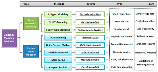
Figure 1.
Comparison of different digital 3D modeling methods.
Physics-based modeling [5] considers the basic physics of surface deformation. Compared with polygon modeling and NURBS modeling, it has the ability to create a more realistic look. Physics-based modeling methods include finite element method [6], finite difference method [7], finite volume method [8], mass-spring systems [9], the meshless method [10], coupled particle systems [11] and simplified deformation models for modal analysis [12].
PDE geometric modeling was pioneered by Bloor and Wilson [13] in computer graphics three decades ago. Since then, PDE methods have been developed to tackle various geometric modeling problems, such as surface modeling [14,15], surface design [16], and solid modeling [17], and are used to represent high-speed train head models [18] and optimize aerodynamic performance of high speed train heads [19]. One major advantage is that the differential operator of PDE can generate smooth surfaces [18]. Another advantage of using the PDE approach is that PDE surfaces can be generated by intuitive manipulation of the relatively small set of boundary conditions for PDE [20]; it can transform geometric modeling problems into boundary value PDE problems. Therefore, the PDE modeling method can obtain continuous smooth surfaces without manual work to stitch adjacent patches together.
Elliptic cross sections have been used in sweeping surfaces to describe human shapes [21]. Surface generation from cross-sections is used in many applications, especially in medical visualization. Some illustrative examples include human body 3D visualization with 2D computed tomography (CT) slices [22] or magnetic resonance imaging (MRI) data [23]. Different methods have been developed to reconstruct 3D models or surfaces from cross sections or point clouds [24,25,26,27]. A method for modeling and deforming the human arm and leg by using cross section ellipses and displacement diagrams is proposed in [28]. Another method dealing with curve networks of arbitrary shape and arbitrary topology with arbitrary direction about non-parallel cross sections is reported in [29]. Barton et al. [30] presented an approach to detect if a surface can be represented by the sweeping of a planar profile or not. It shows applications in functional architectural design. Kovács and Várady [31] proposed an algorithm to detect and reconstruct the profile curves from the property that they are principal curvature lines. Barton et al. [32] studied the evolution of an arc spline curve which constitutes an effective discretization of smooth curves.Recently an analytical mathematical representation of cross section curves including generalized ellipses, generalized elliptic curves and composite generalized elliptic segments was proposed, and surfaces were reconstructed from the curves in [33].
3. Algorithm Overview
Figure 2 shows the overall algorithm of our proposed approach. It consists of two steps: curve fitting and the creation of continuous PDE surfaces.
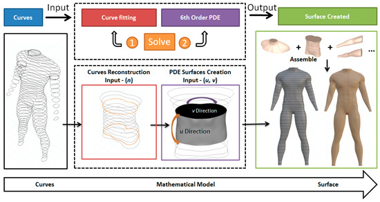
Figure 2.
Overall proposed algorithm.
Before curve fitting, cross section curves of 3D models are created. Four different methods can be used to generate cross section curves. The first method is to manually draw cross section curves by artists or modelers. The second method is to extract the contour of computed tomography slices. The third method is to slice 3D surface models and obtain 2D cross section curves. And the last method is to reconstruct cross section curves from point clouds.
In the first step, i.e., curve fitting, we use generalized elliptic curves to approximate and reconstruct each of the cross section curves. Then these cross section curves are changed into an analytical mathematical expression with few undetermined constants. We call it a generalized elliptic curve. Through this simple procedure, we can get some smooth curves as well as achieve an adequate trade-off between the approximation errors and the amount of data required to approximate cross section curves. It works well on complicated curve-based models with smooth cross-sections. In other words, the ground truth closed curves are defined by few coefficients involved in the mathematical expression of generalized elliptic curves, which will be used in the following processes.
In the second step, continuous PDE surface patches are constructed from generalized elliptic curves obtained in the previous step. A vector-valued sixth-order partial differential equation is proposed for this purpose and an accurate closed form solution is obtained from the vector-valued sixth-order partial differential equation, which is used to interpolate the generalized elliptic curves. The interpolation operation generates a PDE surface patch. Since two adjacent PDE surface patches share three same cross section curves or share the same curve, first partial derivatives, and the second partial derivatives on their joint boundary, continuity between two adjacent PDE surface patches is naturally achieved.
3.1. Curve Fitting
Figure 3 shows the first step of the algorithm. In the figure, the ground truth curves are highlighted in blue, the generalized elliptic curves defined by Equation (1) below are in red, and indicates the number of Fourier series terms in Equation (1). First, we use the cross-section curves of a 3D model as input. For each ground truth cross-section curve (blue), we use a generalized elliptic curve (red) to fit it. The mathematical expression of generalized elliptic curves is given in Equation (1). In doing so, the ground truth curves are now defined by the few coefficients involved in the mathematical expression of the generalized elliptic curves.
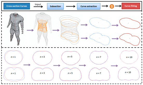
Figure 3.
Curve fitting example. The ground truth curves are shown in blue and fitted generalized elliptic curves are in red.
The figure above shows that the blue ground truth curves are approximated by the red generalized elliptic curves very well and the errors between them are very small. When , large differences between the ground truth curves and the generalized elliptic curves can be seen. When increases, the differences become smaller and smaller. When , visiable differences between the ground truth curves and the generalized elliptic curves disappear.
Good fitting accuracy is also demonstrated by the data given in Table 1. When , the average and maximum errors are 0.044169 and 0.065371, respectively. When is raised to 7, they are reduced to 0.001767 and 0.005312, which are small. When the terms are further increased, the errors will be reduced further. They indicate that by using different terms in Equation (1), the fitting accuracy can be controlled and ground truth curves can be approximated accurately by generalized elliptic curves.

Table 1.
Errors of curve fitting.
Because there are no sharp points in organic shapes like a human body, through this process we can get smooth curves and eliminate input sharp points if they exist. By doing so, we can also fix errors in an artist’s drawn models and improve the final results. The mathematical expression of generalized elliptic curves can be written as
where and are undetermined constants, which are determined by using Equation (1) to fit cross section curves represented with discrete points. As shown in Equation (1), the parameter could be set to different numbers in order to get different resolutions and degree of approximation.
3.2. Creation of Continuous PDE Surfaces
According to [32], “there is no restriction upon the type and order of the PDE to be solved” and “elliptic PDEs have been chosen to develop this technique since this kind of PDE is regarded as an averaging process throughout the entire surface”. In this paper, an elliptic PDE will be introduced to develop a 3D modelling method.
When a continuous PDE surface patch is created from known boundary conditions on two boundaries, it should satisfy the position functions and the first and second partial derivatives on the two boundaries. Therefore, there are six boundary conditions in total. It is known that the closed form solution of a sixth-order partial differential equation involves six undetermined constants which can be used to exactly satisfy the six boundary conditions. Therefore, in order to achieve continuity between two adjacent PDE surface patches, the following vector-value sixth-order partial differential equation is proposed to define PDE surface patches:
According to the above Equation (1), the solution to the partial differential Equation (2) can be taken to be:
In the above Equations (3)–(5), the undetermined functions and and are derived in Appendix A, which can be written as Equations (6), (7), and (8) below, respectively.
For ,
For ,
In what follows, we use the solution for the case , i.e., Equations (3)–(5) whose undetermined functions are determined by Equations (6) and (8), to reconstruct 3D shapes consisting of continuous PDE surface patches.
Twelve curves shown in Figure 3 are used to demonstrate how to reconstruct three PDE surface patches with continuity. The mathematical equations for 12 curves are:
As shown in Figure 4, the six curves are used to construct the first PDE surface patch (Patch 1). Then, two different methods are used to construct PDE surface patch 2 and patch 3 with continuity. For curve , of Patch 1 is the same as of Patch 2. Similarly, for curve , of Patch 1 is the same as of Patch 3. Curve is at of Patch 2 and is at of Patch 3.
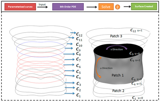
Figure 4.
Surface creation example. The six curves − (red) are used to construct the PDE surface patch 1.
The first method uses the six curves to construct the PDE surface patch 1, the curves to construct the PDE surface patch 2, and the six curves to construct the PDE surface patch 3. With this construction method, the patch 1 and patch 2 at the curve and the patch 1 and patch 3 at the curve achieve up to continuity.
The second method calculates the first and second partial derivatives of the PDE surface patch 1 at the curves and , and use the curves and the first and second partial derivatives of the PDE surface patch 1 at the curves to construct the PDE surface patch 2, and the curves and the first and second partial derivatives of the PDE surface patch 1 at the curves to construct the PDE surface patch 3. With this construction method, the patch 1 and patch 2 at the curve and the patch 1 and patch 3 at the curve also achieve continuity. The first partial derivatives can be obtained below from Equations (6) and (8).
And the second partial derivatives can be derived from the above Equations (10) and (11) and have the forms below
Substituting into Equations (10)–(13), we obtain the first and second partial derivatives of the PDE surface patch 2 at . They together with the curves are used to construct the PDE surface patch 2.
Substituting into Equations (10)–(13), we obtain the first and second partial derivatives of the PDE surface patch 3 at . They together with the curves are used to construct the PDE surface patch 3.
3.2.1. PDE Surface Patch 1 Creation
The six curves for Patch 1 are at ,,,,, and . At these positions, the PDE surface patch 1 passes through the six curves, which gives six equations for x component, y component, and z component.
For the middle PDE surface patch 1, we introduce the superscript P1 into Equations (3)–(5) and change them into:
The middle PDE surface patch 1 is created from 6 curves . The PDE surface Patch 1 passes through the Curves , which gives the following equations.
where the superscript “P1” indicates the first PDE surface patch.
Although the values of the parametric variable are taken to be uniform, i.e., (), the values of can be arbitrary, i.e., uniform or nonuniform since the function for the component involves six undetermined constants to exactly satisfy arbitrary variations defined by the six values of .
The above Equation (15) can be changed into the following three groups of equations
For the PDE surface patch 1, we introduce the superscript P1 into Equations (6) and (8) and obtain:
Substituting Equation (19) into the above Equation (16), the first group of equations is changed into below
Substituting the first of Equation (20) into the above Equation (17), the second group of equations is changed into below
Substituting the second of Equation (32) into the above Equation (30), the third group of equations is changed into below
Solving Equation (21), we obtain the undetermined constants (. Solving Equation (22), we obtain the undetermined constants (. Solving Equation (23), we obtain the undetermined constants (. After that, substituting ( into Equation (19), and ( into Equation (20), and then substituting Equations (19) and (20) into Equation (14), we obtain the PDE surface patch 1.
3.2.2. Creation of PDE Surface Patch 2
Two methods can be used to create the bottom PDE surface patch 2. The first method uses the six curves to create the PDE surface patch 2, and the second method uses the curves and the first and second partial derivatives of the PDE surface patch 1 at the curve . For creation of the bottom PDE surface patch 2 from 6 curves , the three curves are shared by both PDE surface Patches 1 and 2 to ensure continuity on the curve .
With the first method, we use to replace , and , and (), and and () to replace (), and and (). Same as the above treatment, we obtain . With the obtained and we create the PDE surface patch 2 between , which achieves up to continuity with the PDE surface patch 1 at of the PDE surface patch 2, which is on the curve .
With the second method, the PDE surface patch 2 shares the same first and second partial derivatives with the PDE surface patch 1 on the curve , and the PDE surface patch 2 passes through the curves . According to these requirements, we obtain the following equations:
where
The undetermined functions and and involved in Equation (26) are determined by solving Equations (24) and (25). The details of solving Equations (24) and (25) are given in Appendix B.
With the obtained and , we create the PDE surface patch 2 between with Equation (26), which achieves up to continuity with the PDE surface patch 1 at of the PDE surface patch 2.
3.2.3. Creation of PDE Surface Patch 3
With the same method as creating PDE surface patch 2, we can create PDE surface patch 3, which can be written as the following equations.
4. Results
The above method and corresponding mathematical equations have been implemented using C++. The implemented computer program consists of two parts. The first part determines the coefficients involved in Equation (1) by fitting it to cross section curves, and the second part determines the undetermined coefficients ( and and ( for the PDE surface patch 1, ( and and ( for the PDE surface patch 2, and ( and and ( for the PDE surface patch 3.
Figure 5 gives an example of creating the parts of shoulder, body, left arm and leg with the above obtained PDE surface patches.
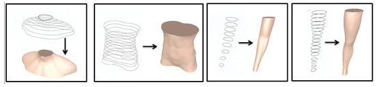
Figure 5.
The cross section curves and created human body parts.
Figure 6 shows the cross section curves of the human body and the reconstructed human body in front and side views. The reconstructed and rendered human body models show that our method can obtain smooth models without any manual operations to stitch adjacent patches together.
Figure 6.
The cross section curves of the human body and the created human body model in front and side views using continues PDE method.
Figure 7 shows smooth models of a vase, a horse belly, elephant front legs, and an elephant nose generated from vertical or horizontal cross section curves by using the method proposed in this paper.
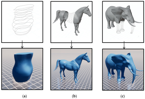
Figure 7.
Surface shape generation from cross section curves by using the method proposed in this paper. (a) a smooth vase model, (b) a horse belly model, (c) front leg and nose models of an elephant.
5. Conclusions
We have developed a PDE-based modelling method to create 3D models in this paper. Fourier series have been used to define generalized elliptic curves which can approximate ground-truth cross section curves with few coefficients and high accuracy. A vector-valued sixth-order partial differential equation has been proposed to construct 3D models from cross section curves and achieve continuity between two adjacent PDE surface patches. The accurate closed form solution to the vector-valued sixth-order partial differential equations has been derived, and the undetermined constants involved in the closed form solution have been determined by interpolating cross section curves while keeping continuity between two adjacent PDE surface patches. A number of examples have been presented to demonstrate the application of the proposed method in creating 3D models from cross section curves.
With the help of the physics-based analytical mathematical solution, a very complicated cross section curve can be represented with few variables. Compared with the polygon modeling, the proposed approach generates complicated and smooth surface models with fewer design variables and requires less hardware storage. In comparison with NURBS modeling, the proposed method has no continuous problem between different patches, which leads to the advantages of saving manual operations and reducing geometric modelling workload and time.
Moreover, the presented examples show that our method is accurate and effective in creating a 3D surface model from cross section curves. Because of fewer variables and analytical mathematical expression, the proposed approach is applicable to many applications involving heavy calculations such as machine learning-based shape reconstruction and computer animation and situations such as level of detail where different resolutions of a geometric model are used for different visual requirements.
The limitation of our method is additional processing of 3D models with more than one branch. For this situation, 3D models are segmented into parts. Each part is created with the method proposed in this paper. When two adjacent part models cannot be directly connected together, a transition surface is created to connect the two adjacent part models together. The transition surface is defined by two boundary curves respectively on the adjacent part models and the continuity requirements on the two boundary curves. The blending method proposed in [33] can be used to create the transition surface, which smoothly connects the two adjacent part models together with continuity.
Our work opens up several directions for future work. The first direction is input data processing. Although the method of reconstructing cross section curves from point clouds is mentioned in Section 3, how to obtain reconstructed cross section curves has not been discussed in this paper. In our following work, we will develop a new method to reconstruct Fourier series-represented cross section curves from point clouds.
The second direction is to extend the proposed method to more modelling applications of organic models and smooth man-made models. These organic models and smooth man-made models include non-human animals such as horses, bell peppers, vases, mountain contours, and streamlined aircrafts, trains and cars. We will investigate these modelling applications in our following work.
This paper discusses 3D modelling based on cross section curves. Actually, the method proposed in this paper can be extended to deal with spatial curves. In this case, the position component is also the function of the parametric variables and . The undetermined constants involved in the component function can be determined with the same method as the one used to determine the undetermined constants involved in the and component functions.
Author Contributions
Conceptualization, L.Y. and H.F.; validation, S.B., H.F. and O.L.; writing—original draft preparation, H.F. and L.Y.; writing—review and editing, H.F., S.B., A.I., J.M. and L.Y.; visualization, H.F. and E.C.; supervision, A.I., L.Y., J.M. and J.J.Z.; funding acquisition, A.I., L.Y. and J.J.Z. All authors have read and agreed to the published version of the manuscript.
Funding
This research is supported by the PDE-GIR project, which has received funding from the European Union Horizon 2020 Research and Innovation Programme under the Marie Skodowska-Curie grant agreement No 778035. Andres Iglesias also thanks the project TIN2017-89275-R funded by MCIN/AEI/10.13039/501100011033/FEDER “Una manera de hacer Europa”. And Haibin Fu is grateful for a scholarship from the Rabin Ezra Scholarship Trust.
Institutional Review Board Statement
Not applicable.
Informed Consent Statement
Not applicable.
Conflicts of Interest
The authors declare that they have no conflict of interest.
Appendix A. Determination of the Undetermined Functions A
Substituting Equation (3) into Equation (2), we have
Substituting Equation (4) into Equation (2), we have
Substituting Equation (5) into Equation (2), we have
The above Equations (A1)–(A3) can be rewritten as the following equations
The solution to the ordinary differential Equation (A4) is:
Substituting into the ordinary differential Equation (A5), we obtain the following characteristic equation:
When ,
For , we have
where
For , we have
From the obtained six roots , the solution to the differential Equation (A5) is obtained as:
The same method is applied to Equation (A6) to obtain
When ,
where is the imaginary unit.
Cubic roots of the imaginary unit are: , and . Substituting them into Equation (A11), we obtain the following six roots.
From , we obtain
where
From , we obtain
From the obtained six roots , the solution to the differential Equation (A5) is obtained as:
Using the same method to solve Equation (A6), we obtain
Appendix B. Determination of the Undetermined Functions B
In order to determine the undetermined functions and and , we first calculate the first and second partial derivatives of the PDE surface patch 1 at , i.e., on the curve .
Substituting Equations (14) and (26) into Equation (24), we obtain the following equations describing the continuity of the first and second partial derivatives.
Equalizing the coefficients of the constant terms, the terms, and the terms, respectively, the above equations are changed into:
Introducing the superscript P1 into Equations (10) and (11) and setting , we obtain the following equations:
Introducing the superscript P1 into Equations (12) and (13) and setting , we obtain the following equations:
Introducing the superscript P2 into Equations (10) and (11) and setting , we obtain the following equations:
Introducing the superscript P2 into Equations (12) and (13) and setting , we obtain the following equations:
Substituting Equations (A19), (A21), (A23) and (A25) into Equation (A17), the following equations are obtained.
Substituting Equations (A20), (A22), (A24) and (A26) into Equation (A18), the following equations are obtained.
Substituting Equation (26) into Equation (25), the four equations in Equation (25) are changed into the following ones:
The above Equation (A30) can be changed into the following three groups of equations
where (.
Following the same method used to obtain Equations (21)–(23), we obtain the following equations from Equations (A31)–(A33).
Solving the six equations in Equations (A27) and (A34), we determine the six undetermined constants (. Solving the six equations in Equations (A28) and (A35), we determine the six undetermined constants (. Solving the six equations in Equations (A29) and (A36), then we determine the six undetermined constants (.
References
- Russo, M. Polygonal Modeling: Basic and Advanced Techniques; Wordware Pub.: Plano, TX, USA, 2006; ISBN 9781598220070. [Google Scholar]
- Piegl, L.; Tiller, W. The NURBS Book; Springer Science & Business Media: Berlin/Heidelberg, Germany, 2012; ISBN 9783540550693. [Google Scholar]
- Farin, G. Curves and Surfaces for Computer-Aided Geometric Design: A Practical Guide; Elsevier: Amsterdam, The Netherlands, 2014; ISBN 9780122490521. [Google Scholar]
- Bischoff, S.; Kobbelt, L. Teaching meshes, subdivision and multiresolution techniques. Comput.-Aided Des. 2004, 36, 1483–1500. [Google Scholar] [CrossRef]
- Nealen, A.; Müller, M.; Keiser, R.; Boxerman, E.; Carlson, M. Physically Based Deformable Models in Computer Graphics. In Computer Graphics Forum; Blackwell Publishing Ltd.: Oxford, UK, 2006; Volume 25, pp. 809–836. [Google Scholar] [CrossRef]
- Li, Z.-C.; Chang, C.-S. Boundary penalty finite element methods for blending surfaces, III. Superconvergence and stability and examples. J. Comput. Appl. Math. 1999, 110, 241–270. [Google Scholar] [CrossRef] [Green Version]
- Chaudhry, E.; Bian, S.J.; Ugail, H.; Jin, X.; You, L.H.; Zhang, J.J. Dynamic skin deformation using finite difference solutions for character animation. Comput. Graph. 2015, 46, 294–305. [Google Scholar] [CrossRef] [Green Version]
- Cornford, S.L.; Martin, D.F.; Graves, D.T.; Ranken, D.F.; Le Brocq, A.M.; Gladstone, R.M.; Payne, A.J.; Ng, E.G.; Lipscomb, W.H. Adaptive mesh, finite volume modeling of marine ice sheets. J. Comput. Phys. 2013, 232, 529–549. [Google Scholar] [CrossRef]
- Liu, T.; Bargteil, A.W.; O’Brien, J.F.; Kavan, L. Fast simulation of mass-spring systems. ACM Trans. Graph. 2013, 32, 1–7. [Google Scholar] [CrossRef]
- Donning, B.M.; Liu, W.K. Meshless methods for shear-deformable beams and plates. Comput. Methods Appl. Mech. Eng. 1998, 152, 47–71. [Google Scholar] [CrossRef]
- Taniguchi, T.; Sawada, S. Stochastic boundary approaches to many-particle systems coupled to a particle reservoir. Phys. Rev. E 2017, 95, 012128. [Google Scholar] [CrossRef] [Green Version]
- Bai, J.; Zhang, J.; Jin, S.; Du, K.; Wang, Y. A multi-modal-analysis-based simplified seismic design method for high-rise frame-steel plate shear wall dual structures. J. Constr. Steel Res. 2021, 177, 106484. [Google Scholar] [CrossRef]
- Bloor, M.I.G.; Wilson, M.J. Generating blend surfaces using partial differential equations. Comput.-Aided Des. 1989, 21, 165–171. [Google Scholar] [CrossRef]
- Bloor, M.I.G.; Wilson, M.J. Using partial differential equations to generate free-form surfaces. Comput.-Aided Des. 1990, 22, 202–212. [Google Scholar] [CrossRef]
- Sheng, Y.; Sourin, A.; Castro, G.G.; Ugail, H. A PDE method for patchwise approximation of large polygon meshes. Vis. Comput. 2010, 26, 975–984. [Google Scholar] [CrossRef]
- Ugail, H.; Bloor, M.I.G.; Wilson, M.J. Techniques for interactive design using the PDE method. ACM Trans. Graph. 1999, 18, 195–212. [Google Scholar] [CrossRef]
- Ahmat, N.; Ugail, H.; Castro, G.G. Method of modelling the compaction behaviour of cylindrical pharmaceutical tablets. Int. J. Pharm. 2011, 405, 113–121. [Google Scholar] [CrossRef] [PubMed]
- Wang, S.B.; Xia, Y.; Wang, R.B.; You, L.H.; Zhang, J.J. Optimal NURBS conversion of PDE surface-represented high-speed train heads. Optim. Eng. 2019, 20, 907–928. [Google Scholar] [CrossRef] [Green Version]
- Wang, S.B.; Wang, R.B.; Xia, Y.; Sun, Z.; You, L.H.; Zhang, J.J. Multi-objective aerodynamic optimization of high-speed train heads based on the PDE parametric modelling. Struct. Multidiscip. Optim. 2021, 64, 1285–1304. [Google Scholar] [CrossRef]
- Wang, S.B.; Xiang, N.; Xia, Y.; You, L.H.; Zhang, J.J. Real-time surface manipulation with C1 continuity through simple and efficient physics-based deformations. Vis. Comput. 2021, 37, 2741–2753. [Google Scholar] [CrossRef]
- Gonzalez, C.G.; Ugail, H.; Willis, P.; Palmer, I.J. A survey of partial differential equations in geometric design. Vis. Comput. 2008, 24, 213–225. [Google Scholar] [CrossRef] [Green Version]
- Chen, C.; Sheng, Y.; Li, F.; Zhang, G.; Ugail, H. A PDE-based head visualization method with CT data. Comput. Animat. Virtual Worlds 2015, 28, e1683. [Google Scholar] [CrossRef]
- Ma, A.; Yang, R.; Ning, H.; Bai, H.; Li, L.; Wu, X. 3D scalp extraction and reconstruction of MRI brain images. J. Comput. Appl. 2013, 33, 1439–1442. [Google Scholar] [CrossRef]
- Hyun, D.-E.; Yoon, S.-H.; Chang, J.-W.; Seong, J.-K.; Kim, M.-S.; Jüttler, B. Sweep-based human deformation. Vis. Comput. 2005, 21, 542–550. [Google Scholar] [CrossRef]
- Xu, F.; Mueller, K. Real-time 3D computed tomographic reconstruction using commodity graphics hardware. Phys. Med. Biol. 2007, 52, 3405–3419. [Google Scholar] [CrossRef] [PubMed]
- Yoon, S.-H.; Kim, M.-S. Sweep-based Freeform Deformations. In Computer Graphics Forum; Blackwell Publishing Ltd.: Oxford, UK, 2006; Volume 25, pp. 487–496. [Google Scholar] [CrossRef]
- Farin, G.; Hoschek, J.; Kim, M.-S. Reverse engineering. In Handbook of Computer Aided Geometric Design; Elsevier: Amsterdam, The Netherlands; Boston, MA, USA, 2002; Volume 26, ISBN 9780444511041. [Google Scholar]
- Li, O.; Chaudhry, E.; Yang, X.; Fu, H.; Fang, J. Composite generalized elliptic curve-based surface reconstruction. In International Conference on Computational Science; Springer: Cham, Switzerland, 2021. [Google Scholar]
- Liu, L.; Bajaj, C.; Deasy, J.O.; Low, D.A.; Ju, T. Surface Reconstruction From Non-parallel Curve Networks. In Computer Graphics Forum; Blackwell Publishing Ltd.: Oxford, UK, 2008; Volume 27, pp. 155–163. [Google Scholar] [CrossRef] [Green Version]
- Barton, M.; Pottmann, H.; Wallner, J. Detection and reconstruction of freeform sweeps. In Computer Graphics Forum; Blackwell Publishing Ltd.: Oxford, UK, 2014; Volume 33, pp. 23–32. [Google Scholar] [CrossRef]
- Kovács, I.; Várady, T.; Cripps, R. Reconstructing swept surfaces from measured data. In The Mathematics of Surfaces XIV; Cripps, R., Ed.; IMA: Tarrytown, NJ, USA, 2013; pp. 327–344. [Google Scholar]
- Barton, M.; Shi, L.; Kilian, M.; Wallner, J.; Pottmann, H. Circular arc snakes and kinematic surface generation. In Computer Graphics Forum; Blackwell Publishing Ltd.: Oxford, UK, 2013; Volume 32, pp. 1–10. [Google Scholar] [CrossRef] [Green Version]
- You, L.H.; Comninos, P.; Zhang, J.J. PDE blending surfaces with C2 continuity. Comput. Graph. 2004, 28, 895–906. [Google Scholar] [CrossRef]
Publisher’s Note: MDPI stays neutral with regard to jurisdictional claims in published maps and institutional affiliations. |
© 2022 by the authors. Licensee MDPI, Basel, Switzerland. This article is an open access article distributed under the terms and conditions of the Creative Commons Attribution (CC BY) license (https://creativecommons.org/licenses/by/4.0/).