GeoStamp: Detail Transfer Based on Mean Curvature Field

Abstract

A shape detail transfer is the process of extracting the geometric details of a source region and transferring it onto a target region. In this paper, we present a simple and effective method, called GeoStamp, for transferring shape details using a Poisson equation. First, the mean curvature field on a source region is computed by using the Laplace–Beltrami operator and is defined as the shape details of the source region. Subsequently, the source and target regions are parameterized on a common 2D domain, and a mean curvature field on the target region is interpolated by the correspondence between two regions. Finally, we solve the Poisson equation using the interpolated mean curvature field and the Laplacian matrix of the target region. Consequently, the mean curvature field of the target region is replaced with that of the source region, which results in the transfer of shape details from the source region to the target region. We demonstrate the effectiveness of our technique by showing several examples and also show that our method is quite useful for adding shape details to a surface patch filling a hole in a triangular mesh.

1. Introduction

Owing to their simplicity and hardware-accelerated rendering facilities, triangular meshes have been widely used to represent the shape of three-dimensional (3D) objects in computer graphics and real-time 3D applications. During the last several decades, the modeling and deformation of a triangular mesh has been an important research subject in geometric modeling and processing owing to its ever widening range of applications in industrial and artistic design [1]. Among these techniques, creating shape details is an essential process for enhancing the realism of 3D objects. However, manually creating shape details with existing modeling tools is still a tedious and time-consuming task. Therefore, several methods [2,3,4,5] have been proposed for reusing existing shape details instead of creating them from scratch. In general, detail transfer refers to the process of extracting the shape details from one region and transferring it to another.

Geometric detail is an intrinsic property of a surface; thus, it would be desirable to be represented in a local coordinate system rather than the absolute position or orientation in 3D space. The Laplacian coordinates for a vertex are defined as a displacement vector from the centroid of its neighboring vertices, which provides the intrinsic representation of a triangular mesh. Based on this representation, Sorkine et al. [5] introduced a coating vector as the difference between two Laplacian coordinates of the original surface and its smooth version and developed several mesh-editing operations, such as the transfer of geometric details and the transplanting of a partial surface onto another surface. Although the coating vectors can effectively be used to represent geometric details, their orientations should be handled carefully when transferred to other regions.

In this paper, we also aim to transfer the geometric details from a source region to a target region. However, we take a slightly different approach to this problem by employing a mean curvature field to represent the shape details of a source region. Compared with the coating vectors [5], the computation of a mean curvature field is quite simple and computationally efficient because it does not require a smooth version of the original surface. Moreover, we do not need to consider the orientation of the shape details when applied to a target region. Consequently, the problem of a detail transfer simply boils down to finding the solution of a Poisson equation, which can be efficiently solved through stable numerical techniques.

The overall process of the proposed method is illustrated in Figure 1. First, the mean curvature field on a source region of a triangular mesh is computed from the Laplacian of the coordinates of the mesh vertices (Figure 1a), and a correspondence between the source and target regions is then established by parameterizing two regions over a common 2D domain (Figure 1b). Subsequently, the mean curvature field on the target region is interpolated by the correspondence between two regions (Figure 1c). Finally, we solve a Poisson equation using the interpolated mean curvature field and Laplacian matrix of the target region. The result with the transferred details is shown in Figure 1d, where the target region is reconstructed from the interpolated mean curvature field of the source region.

The main contributions of our method can be summarized as follows:

• Robustness: We formulate the transfer of the shape details as finding the solutions to a Poisson equation of a sparse symmetric linear system. By employing an efficient numerical solver, we can guarantee robust solutions to the problem.
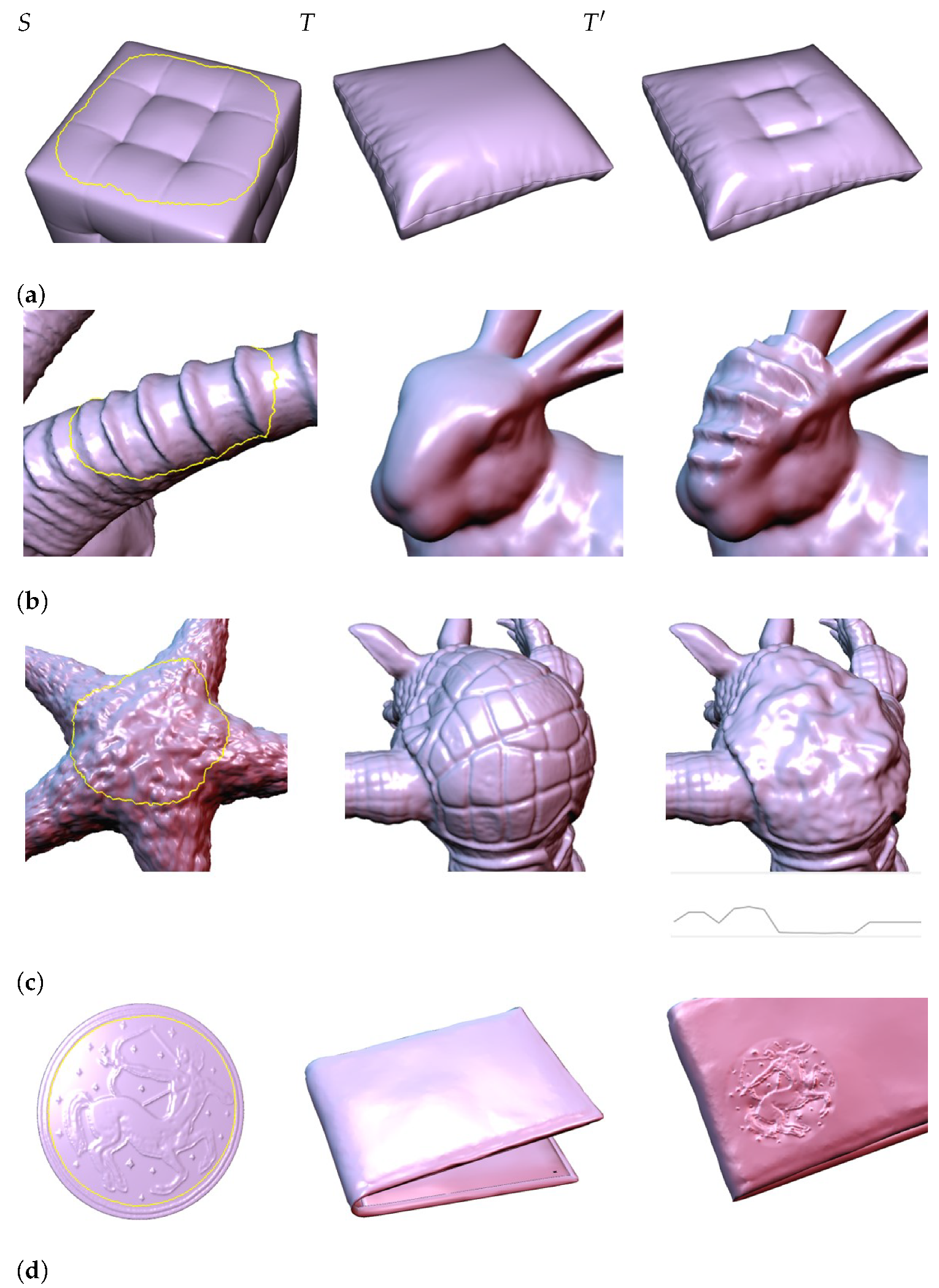
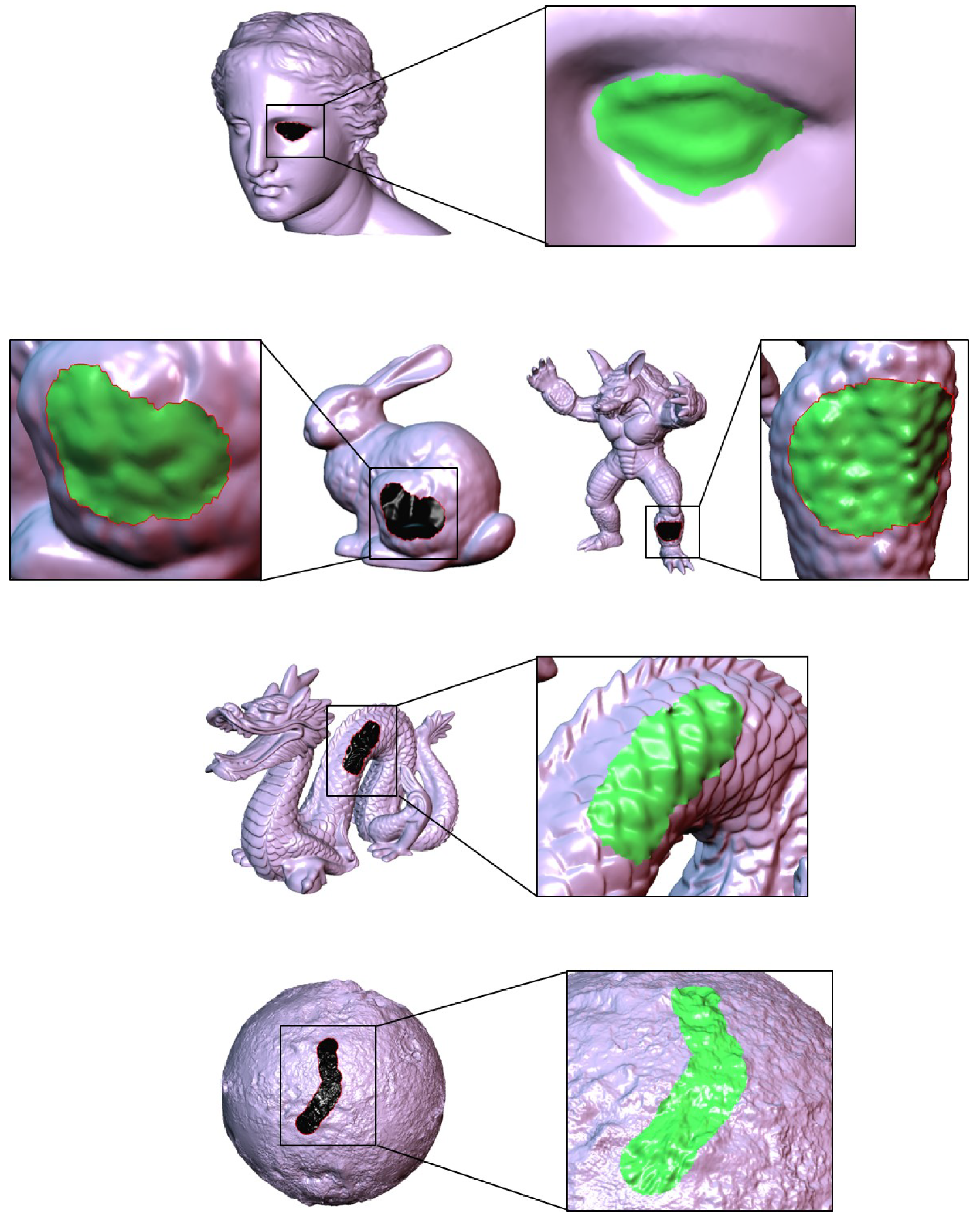
• Effectiveness: By analyzing the mean curvatures, any shape details such as regular patterns or irregular bumps can be effectively transferred to a target region. Moreover, our method can effectively and easily be combined with conventional methods such as the hole-filling of a triangular mesh to generate sophisticated results to match the shape details around a hole (see Supplementary Video).
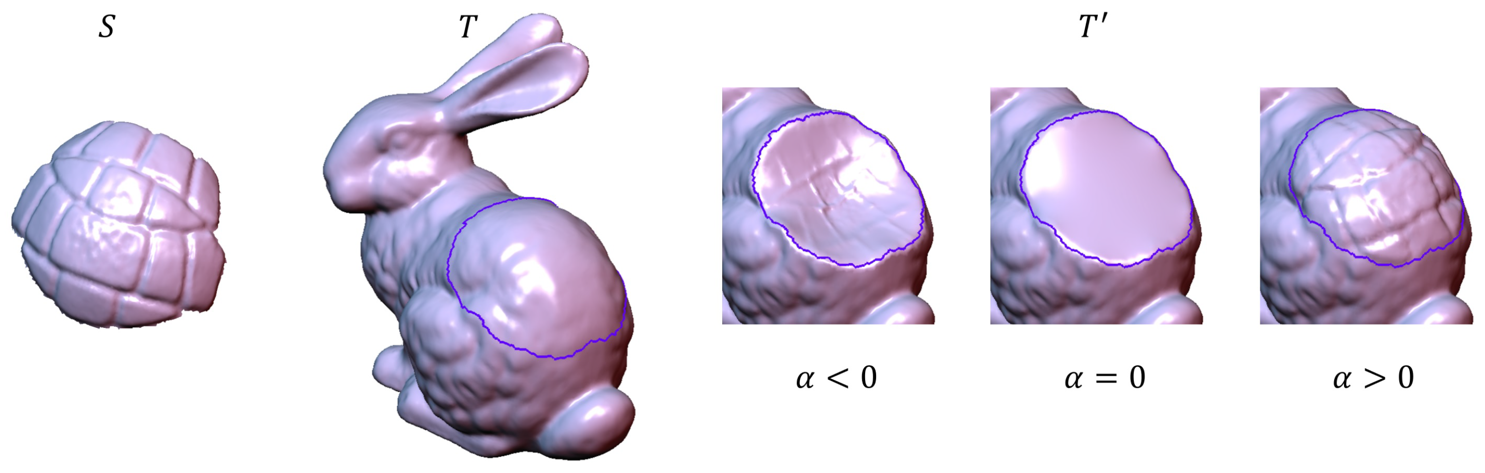
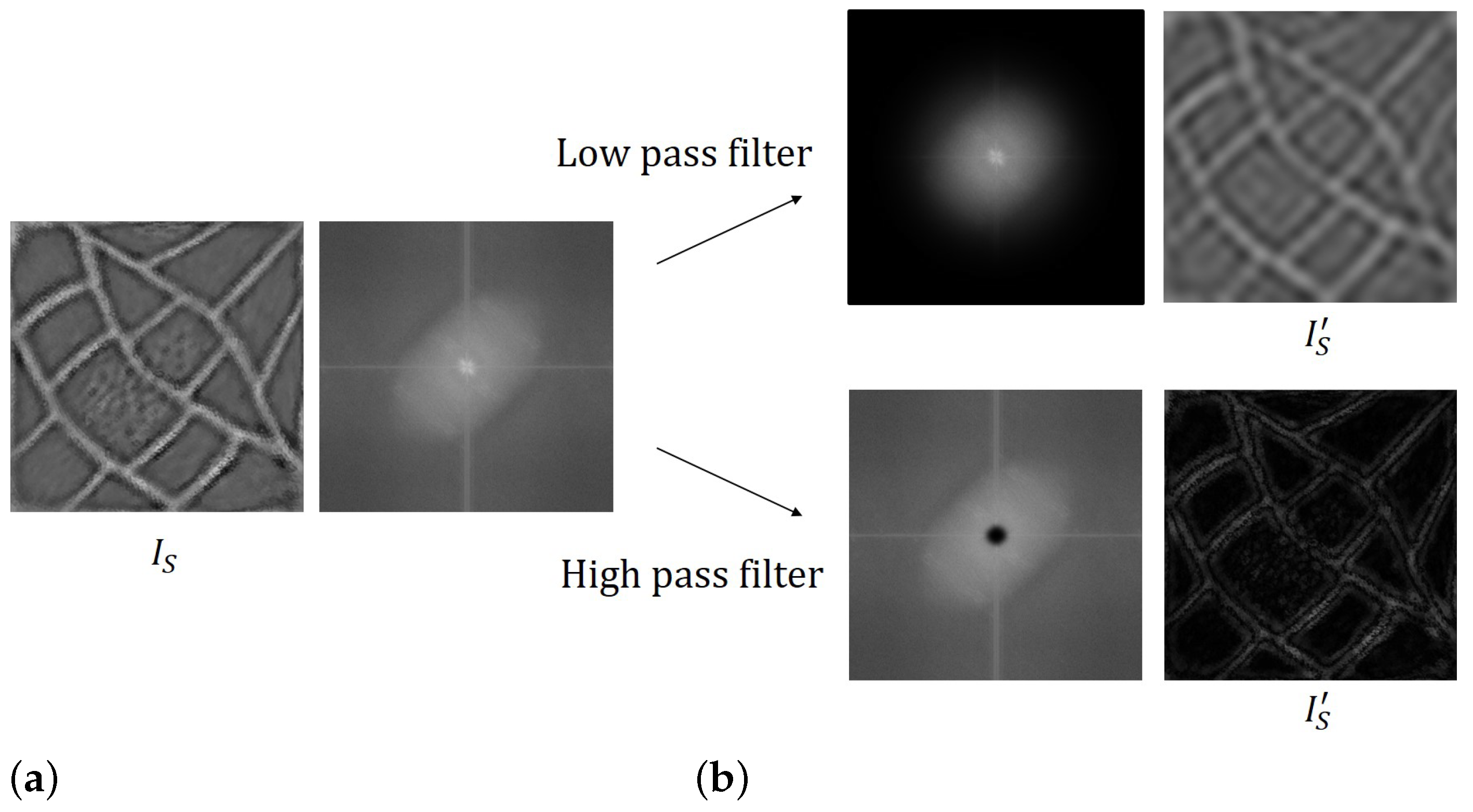
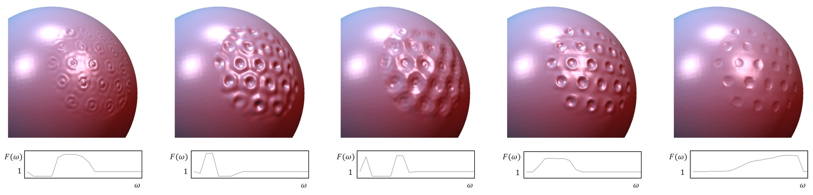
• Controllability: Our method provides the user with several control parameters for the shape detail intensity and orientation. The shape details can be thought of as a grayscale image on the parameter domain and thus analyzed within the frequency domain by applying a fast Fourier transformation (FFT). In the frequency domain, the user can edit the shape details interactively and transfer them to the target region in the spatial domain.

The paper is organized as follows. In Section 2, we briefly review recent work on the detail transfer of triangular meshes. Section 3 describes the representation of the shape details of a source region using a mean curvature field. The transfer of the shape details from the source region to a target region is detailed in Section 4, and various experimental results are presented in Section 5. Finally, we conclude the paper and discuss areas of future work in Section 6.

2. Related Work

In this section, we briefly review previous works directly related to our method, which include computations of the discrete differential property and shape detail transfer on a polygonal mesh.

2.1. Discrete Differential Property

Based on the assumption that polygonal meshes can be interpreted as piecewise linear approximations of smooth surfaces, many approaches have been proposed for computing discrete differential properties such as normal vectors and curvatures of the underlying surface directly from the mesh data. Taubin [6] introduced a method for estimating the tensor of the curvature of a surface at the vertices of a polyhedral approximation, and in [7], the author proposed the uniform discretization of the Laplace–Beltrami operator. However, because the uniform Laplace–Beltrami operator only depends on the connectivity of the mesh, it is inappropriate for non-uniform meshes with obtuse angles. Meyer et al. [8] proposed a more accurate discretization of the Laplace–Beltrami operator using a mixed finite element/finite volume method and derived estimates for the mean curvature of mesh vertices. Alternative derivations of the same result are presented in [9,10].

Cojen and Morvan [11] also proposed discrete definitions for the mean and Gaussian curvature and the curvature tensor based on the normal cycle theory and proved that the estimated curvature tensors converge to the true values of the smooth surface under specific sampling conditions. Rusinkiewicz [12] suggested a method for estimating the curvature tensor per triangle based on the vertex normals. They suggested a least-squares fitting of the curvature tensor to the normal variations across the edges of a given triangle. Gatzke and Grimm [13] suggested a technique for building a natural local parameterization of the surface and used it to compute differential properties. Kalogerakis et al. [14] proposed a statistical approach to a curvature estimation that is automatic and operates on discretely sampled surfaces.

In this paper, we employ the discrete Laplace–Beltrami operator proposed by Meyer et al. [8] to compute the discrete mean curvature, which is the de facto standard in computer graphics and is widely used for various geometry processing tasks [15]. However, a more sophisticated method can be used to improve the effectiveness of the proposed method.

2.2. Detail Transfer

Many studies have been conducted on representing the local features or details of a polygonal surface. Alexa [2] introduced the idea of describing a mesh geometry by using differential coordinates. The differential coordinates describe the mesh geometry as relative coordinates in a local coordinate system rather than those in a world coordinate system and are thus quite useful for representing local features or details. Lipman et al. [3] proposed an approach to rotating the differential coordinates according to the orientation of a local frame defined on each vertex and demonstrated that this approach can effectively be used for editing complex detailed meshes while maintaining the shape of the details in their natural orientation. By using differential coordinates for vertices, Sorkine et al. [4,5] developed a technique for transferring geometric details between two polygonal surfaces.

In addition, Biermann et al. [16] proposed a set of algorithms based on multiresolution subdivision surfaces that perform at interactive rates and enable intuitive cut-and-paste operations. They defined the shape details of a source surface as the displacement vectors from a smoothed surface and represent them in a local frame. Liu et al. [17] also proposed an image-based surface detail transfer method that does not require the explicit computations of 3D structures. However, their method is more suitable for image models than 3D triangular meshes. Takayama et al. [18] presented a method for the interactive cloning of 3D geometry. They computed an offset membrane for smoothly stitching a source detail to a target region. Recently, Berkiten et al. [19] proposed a learning detail transfer method based on geometric features. They used metric learning to find a combination of geometric features that predict the detailed map similarities on the source mesh. However, within their method, there are too many factors to consider when representing the geometric features at each vertex.

Our method is similar to [5] in that shape details are extracted from the region of interest and are then transferred into a target region. However, their method is cumbersome because a source region should be smoothed several times for extracting the feature vectors (they used the term coating vector), and the feature vectors need to be rotated correctly when they are transferred onto a target region. By contrast, our method employs a mean curvature field to represent the shape details, which is the scalar field defined on the source region and thus does not require rotating feature vectors when transferred to the target region. Moreover, the transfer mechanism is formulated as a simple Poisson equation while providing a robust solution to our problem. An additional advantage of using a scalar field is that it can be analyzed in the frequency domain and be treated it as an image, allowing various image processing techniques to be directly applied in generating enhanced detail transfer effects.

3. Representation of Shape Details

This section describes how to represent the shape details of a source region S of a triangular mesh $\mathbb{M}$. Let $f:S\to R$ be a scalar function defined on S and $f_i$ be the corresponding value to a vertex ${\mathbf{v}}_i\in S$. The Laplace–Beltrami operator $(\Delta )$ of a function f at vertex ${\mathbf{v}}_i$ is given as [8]:

$$\Delta f_i=\frac{1}{A_i}\sum _{{\mathbf{v}}_j\in N_1\left({\mathbf{v}}_i\right)}\left(\frac{\cot {\alpha }_{i,j}+\cot {\beta }_{i,j}}{2}\right)(f_j-f_i),$$

(1)

where $A_i$ is the local area of ${\mathbf{v}}_i$, and $N_1\left({\mathbf{v}}_i\right)$ is the set of one-ring neighboring vertices of ${\mathbf{v}}_i$ (see Figure 2). Intuitively, $\Delta f_i$ can be interpreted as the average of the weighted differences between $f_i$ and neighboring $f_j$s.

For each vertex ${\mathbf{v}}_i$, we can compute the mean curvature normal vector $\Delta {\mathbf{v}}_i=(\Delta x_i,\Delta y_i,$$\Delta z_i)$ by applying the Laplace–Beltrami operator $(\Delta )$ in Equation (1) to the $x_i,y_i$, and $z_i$ coordinates of ${\mathbf{v}}_i$, respectively [15]. The geometric meaning of $\Delta {\mathbf{v}}_i$ can be interpreted as follows:

$$\Delta {\mathbf{v}}_i=(\Delta x_i,\Delta y_i,\Delta z_i)=2h_i{\mathbf{n}}_i,$$

where $h_i$ is the mean curvature of ${\mathbf{v}}_i$, and ${\mathbf{n}}_i$ is its unit normal vector. The absolute value of the mean curvature $|h_i|$ is computed by $\frac{\parallel \Delta {\mathbf{v}}_i\parallel }{2}$, and its sign can be determined through a user-specified outer normal direction ${\tilde{\mathbf{n}}}_i$ as follows:

$$h_i=\left\{\begin{array}{cc}|h_i|\hfill & \mathrm{if}\Delta {\mathbf{v}}_i·{\tilde{\mathbf{n}}}_i>0,\hfill \\ -|h_i|\hfill & \mathrm{otherwise}.\hfill \end{array}\right.$$

For computational efficiency, the mean curvature normal vectors $\Delta {\mathbf{v}}_i(=2h_i{\mathbf{n}}_i)$ for all vertices can be computed simultaneously as follows:

$$\left[\begin{array}{c}\Delta {\mathbf{v}}_1\\ \Delta {\mathbf{v}}_2\\ ⋮\\ \Delta {\mathbf{v}}_n\end{array}\right]=\left[\begin{array}{c}2h_1{\mathbf{n}}_1\\ 2h_2{\mathbf{n}}_2\\ ⋮\\ 2h_n{\mathbf{n}}_n\end{array}\right]=L_S\left[\begin{array}{ccc}{x}_1& y_1& z_1\\ x_2& y_2& z_2\\ ⋮& ⋮& ⋮\\ x_n& y_n& z_n\end{array}\right],$$

where $L_S$ is the Laplacian matrix of a source region S, and $x_i,y_i$, and $z_i$ are the coordinates of a vertex ${\mathbf{v}}_i\in S$ (refer to [8] for more details). Figure 3a,b show the mean curvature normal vectors thus computed, where $\Delta {\mathbf{v}}_i$ in the concave region points to ${\tilde{\mathbf{n}}}_i$, and $\Delta {\mathbf{v}}_i$ in the convex region points to $-{\tilde{\mathbf{n}}}_i$, according to the sign of $h_i$. In this way, we can efficiently construct the mean curvature field $H_S={\left[\begin{array}{ccccc}{h}_1& \cdots & h_i& \cdots & h_n\end{array}\right]}^T$ on S, which consists of the signed mean curvature $h_i$ of each vertex ${\mathbf{v}}_i$ in S. Figure 3c shows the color-coded signed mean curvature field $H_S$. Finally, we use the mean curvature field $H_S$ to represent the shape details of a source region S and aim to transfer them to a target region T of a triangular mesh.

4. Transferring Shape Details

4.1. Shape Details for Target Region

We aim to transfer the shape details $H_S$ from a source region S to a target region T. However, these regions have different numbers of vertices and connectivity, which makes it quite difficult to transfer $H_S$ to T. To resolve this, we need to construct a correspondence between S and T. Two regions can be parameterized onto any convex region $\mathbb{D}\subset R^2$ using the 2D parameterization based on convex combination [20]. A common choice for $\mathbb{D}$ can be either a unit circle or square, as shown in Figure 4. For the unit square, the user-selected starting vertex is mapped to the origin of $\mathbb{D}$, and the other boundary vertices are parameterized to the boundary of $\mathbb{D}$ depending on the distances from the starting vertex. The 2D coordinates for interior vertices are then determined by a convex combination of neighboring vertices (see Figure 4). Note that different choices of starting vertices produce different parameterization results. Figure 5 illustrates two regions, S and T, parameterized onto the common unit square.

Once the two regions S and T have been parameterized onto a common domain $\mathbb{D}$ (e.g., unit square), we can determine the mean curvature field ${\widehat{H}}_T$ for T. Suppose that a vertex $\mathbf{v}\in T$ is mapped to ${\mathbf{v}}^{\prime }\in \mathbb{D}$ and a triangle $\tau \in S$ is mapped to ${\tau }^{\prime }\in \mathbb{D}$, which contains ${\mathbf{v}}^{\prime }$ (see Figure 5). The mean curvature $\widehat{h}$ for $\mathbf{v}\in T$ can be computed as follows:

$$\widehat{h}=\alpha h_i+\beta h_j+\gamma h_k,$$

where $(\alpha ,\beta ,\gamma )$ are the barycentric coordinates of ${\mathbf{v}}^{\prime }$ with respect to ${\tau }^{\prime }\in D$, and $h_{i\left|j\right|k}$ are the mean curvatures of the corner vertices of $\tau \in S$. In this way, we can create the mean curvature field ${\widehat{H}}_T={\left[\begin{array}{ccccc}{\widehat{h}}_1& \cdots & {\widehat{h}}_i& \cdots & {\widehat{h}}_m\end{array}\right]}^T$ for the target region T, where ${\widehat{h}}_i$ is the interpolated mean curvature for a vertex ${\mathbf{v}}_i\in T$. In the following subsection, we describe how to reconstruct the shape of the target region using ${\widehat{H}}_T$.

4.2. Reconstruction of Target Region

The vertices of T must be repositioned to produce ${\widehat{H}}_T$ created from $H_S$. That is, we need to reconstruct the shape of the target region by using the shape details from S. The reconstruction process can be formulated as a Poisson equation with Dirichlet boundary conditions. In general, the Poisson equation with Dirichlet boundary conditions [21,22] is formulated as follows:

$${\Delta f=b,\mathrm{with}f|}_{\mathsf{\partial }\mathrm{\Omega }}=f^{*}{|}_{\mathsf{\partial }\mathrm{\Omega }},$$

(2)

where $\Delta$ is the Laplace–Beltrami operator, and f and b are scalar functions on a domain $\mathrm{\Omega }$. Usually, f is an unknown variable, b is given, and $f^{*}$ is the boundary condition on $\mathsf{\partial }\mathrm{\Omega }$. When $b=0$, the Poisson equation becomes the Laplace equation $\Delta f=0$, which yields a harmonic field on $\mathrm{\Omega }$. For a triangular mesh, through a linearization followed by discretization based on the finite difference or finite element [23,24], Equation (2) boils down to a linear system.

Let $L_T$ be the Laplacian matrix for a target region T, and ${\widehat{H}}_T$ be the mean curvature field interpolated from $H_S$. The target region can be reconstructed such that its mean curvature field coincides with ${\widehat{H}}_T$ by solving the following Poisson system:

$$L_T\left[\begin{array}{ccc}{x}_1& y_1& z_1\\ x_2& y_2& z_2\\ ⋮& ⋮& ⋮\\ x_m& y_m& z_m\end{array}\right]=\alpha \left[\begin{array}{c}{\widehat{h}}_1{\mathbf{n}}_1\\ {\widehat{h}}_2{\mathbf{n}}_2\\ ⋮\\ {\widehat{h}}_m{\mathbf{n}}_m\end{array}\right],$$

(3)

where $\alpha$ is a user-specified parameter; $x_i,y_i$, and $z_i$ are the unknown coordinates of a vertex ${\mathbf{v}}_i\in T$; and ${\mathbf{n}}_i$ is its unit normal vector. The boundary condition can be realized by fixing the positions of the boundary vertices in T. In general, $L_T$ is sparse and symmetric positive-definite, and thus the solution to Equation (3) can be efficiently found through a Cholesky factorization [25].

Figure 6 shows the result of transferring the shape details from S to T by solving the Poisson system. Note that the source detail $H_S$ can be transferred with different orientations depending on the starting vertex in the parameterization stage. In Equation (3), $\alpha$ controls the strength of the transferring effect. For example, source details $H_S$ are embossed on T if $\alpha >0$, $H_S$ is engraved on T if $\alpha <0$, and, in particular, T is reconstructed by minimizing its area [26] if $\alpha =0$. The target regions reconstructed using various values of $\alpha$ are shown in Figure 7.

Shape details cannot be sufficiently reflected when the resolution of a target region (i.e., the density of the triangles) is significantly lower than that of the source region (see Figure 8b). In such a case, we can perform a preprocessing step to subdivide the target region before the parameterization step. For this, we apply an incremental remeshing technique [27,28,29] to the target region. As shown in Figure 8c, incremental remeshing increases the resolution of the target region to be similar to that of the source region and improves the result of transferring the shape details.

4.3. Controlling Shape Details

As shown in Figure 7, a user can control the effect of a detail transfer by changing the user-specified parameter $\alpha$, which is uniformly applied to ${\widehat{H}}_T$ in Equation (3). However, it does not provide a sophisticated control such as the exaggeration and smoothing of salient geometric features. To support these controls, we apply image-processing techniques to the curvature field $H_S$ of a source region. After normalization followed by quantization, $H_S$ can be considered a grayscale image of the 2D parameter domain. More specifically, to analyze the shape detail within the frequency domain, we create a grayscale image $I_S$ of size $512\times 512$ (see Figure 9a). We then apply a fast Fourier transformation (FFT) to $I_S$ and compute the amplitude of each frequency. Figure 9a shows the result of applying FFT to $I_S$. In the frequency domain, we apply various filtering kernels to $I_S$ and consequently obtain the post-processed shape details $H_S$. For example, we can exaggerate or remove salient geometric features of $H_S$ by increasing or decreasing the amplitudes of high frequencies of $I_S$ (see Figure 10).

Compared with a coating vector [5] or displacement vector [16], representing shape detail as a scalar field offers significant benefits for utilizing conventional image processing techniques. Moreover, shape details are applied along the normal directions of the target region; thus, we do not consider their orientations or directions. In the experimental results, we show various results of a detail transfer based on the control of shape details in frequency domain.

In addition, our method supports the blending of shape details from the source and target regions. Let $H_T={\left[\begin{array}{ccc}{h}_1& \cdots & h_m\end{array}\right]}^T$ be a mean curvature field of a target region computed by applying the Laplace–Beltrami operator to the coordinates of vertices in that region. The right side of Equation (3) can be further extended to blend the shape details ${\widehat{H}}_T$ from the source region and $H_T$ from the target region as follows:

$$L_T\left[\begin{array}{ccc}{x}_1& y_1& z_1\\ x_2& y_2& z_2\\ ⋮& ⋮& ⋮\\ x_m& y_m& z_m\end{array}\right]=\alpha \left[\begin{array}{c}\left((1-\beta ){\widehat{h}}_1+\beta h_1\right){\mathbf{n}}_1\\ \left((1-\beta ){\widehat{h}}_2+\beta h_2\right){\mathbf{n}}_2\\ ⋮\\ \left((1-\beta ){\widehat{h}}_m+\beta h_m\right){\mathbf{n}}_m\end{array}\right],$$

where $\beta$ is a user-specified weight for blending source and target details. Figure 11 shows various blending effects of the source and target details, where the target region with minimal area is obtained when $\alpha =0$, and the original target region is restored when $\alpha =1$ and $\beta =1$.

5. Experimental Results

The proposed technique was implemented on a PC with an Intel i7-10700K CPU, 32GB main memory, and an NVIDIA RTX 2060 graphics card, using the C++ language. In this section, we demonstrate the effectiveness of our method by showing several examples and leveraging it with a conventional hole-filling technique.

Figure 12 shows the effects of the control parameter $\alpha$ in Equation (3) when the shape details of S are transferred to T. The control parameter $\alpha$ mainly influences the global intensity of the shape details rather than sophisticated shape features. To control these features, shape details in the frequency domain are edited by using a user-defined detail transfer function $F\left(\omega \right)$. Figure 13 shows various results of transferring shape details (Figure 12) to a spherical model, where each result is generated by different detail transfer functions. Figure 14 shows additional examples in which the shape details from the four models are transferred to the target regions of different models. Our method supports an interactive control for the effect of detail transfer. As the user changes $\alpha$ or the starting vertex in the parameterization, the target region is reconstructed interactively (see Supplementary Video).

Table 1. Number of vertices on a source and a target region and the computation time (in ms) for a detail transfer for each example.

Examples	# Vertices of Source	# Vertices of Target	Computation Time (in ms)
			Sorkine et al. [5]	Our Method
Figure 14a	4731	4032	345	246
Figure 14b	3507	1039	212	158
Figure 14c	2001	21329	676	521
Figure 14d	37187	46640	4235	2488

compares the computation time of our method with that of Sorkine et al. [5]. We measure the computation time for three steps: the extraction of shape details from a source region, the parameterization of a source and target regions, and the reconstruction of a target region by solving a Poisson equation. Our method is more efficient than that of Sorkine et al. [5] because shape details are not represented by coating vectors but by a simple scalar field, and the orientations of the shape details are automatically determined based on the normal direction of the target region.

To create a hole patch that reflects the shape details around the hole, our method can easily be combined with existing approaches such as the hole-filling technique [30]. As shown in Figure 15, an initial hole patch is constructed by minimizing the curvature variation or thin-plate energy, and the shape details from a source region (around the hole) are transferred to the hole patch to match the shape details around the hole (see Supplementary Video).

6. Conclusions and Future Work

We presented an effective method for transferring the shape details from a source region to a target region of a triangular mesh. Shape details from a source region are represented by the mean curvature field, and the shape details for a target region are interpolated from the source details. For this, we constructed the correspondence between two regions with different geometries and connectivity using 2D parameterization. The target region was then reconstructed from the interpolated shape details by solving the Poisson system while representing the source details. The user can control the effect of the detail transfer by applying image processing techniques to the mean curvature field of the source region, as desired. In the experimental results, we demonstrated the effectiveness of the proposed method by showing several examples of transferring shape details and a hole-filling application. In future work, we will extend our technique so as to blend shape details from multiple regions, and apply sophisticated image processing techniques for editing and enhancing shape details.

References

1. Botsch, M.; Sorkine, O. On linear variational surface deformation methods. IEEE Trans. Vis. Comput. Graph. 2007, 14, 213–230. [Google Scholar] [CrossRef] [PubMed] [Green Version]
2. Alexa, M. Differential coordinates for local mesh morphing and deformation. Vis. Comput. 2003, 19, 105–114. [Google Scholar] [CrossRef]
3. Lipman, Y.; Sorkine, O.; Cohen-Or, D.; Levin, D.; Rossi, C.; Seidel, H.P. Differential coordinates for interactive mesh editing. In Proceedings of the Shape Modeling Applications, Genova, Italy, 7–9 June 2004; pp. 181–190. [Google Scholar]
4. Sorkine, O. Laplacian mesh processing. In Proceedings of the Eurographics 2005—State of the Art Reports. The Eurographics Association, Vienna, Austria, 3–7 May 2005. [Google Scholar]
5. Sorkine, O.; Cohen-Or, D.; Lipman, Y.; Alexa, M.; Rössl, C.; Seidel, H.P. Laplacian surface editing. In Proceedings of the 2004 Eurographics/ACM SIGGRAPH Symposium on Geometry Processing. Association for Computing Machinery, Nice, France, 8–10 July 2004; pp. 175–184. [Google Scholar] [CrossRef] [Green Version]
6. Taubin, G. Estimating the tensor of curvature of a surface from a polyhedral approximation. In Proceedings of the IEEE International Conference on Computer Vision, Cambridge, MA, USA, 20–23 June 1995; pp. 902–907. [Google Scholar]
7. Taubin, G. A signal processing approach to fair surface design. In Proceedings of the 22nd Annual Conference on Computer Graphics and Interactive Techniques, Los Angeles, CA, USA, 6–11 August 1995; pp. 351–358. [Google Scholar]
8. Meyer, M.; Desbrun, M.; Schröder, P.; Barr, A.H. Discrete differential-geometry operators for triangulated 2-manifolds. In Visualization and mathematics III; Springer: Berlin/Heidelberg, Germany, 2003; pp. 35–57. [Google Scholar]
9. Desbrun, M.; Meyer, M.; Schröder, P.; Barr, A.H. Implicit fairing of irregular meshes using diffusion and curvature flow. In Proceedings of the 26th Annual Conference on Computer Graphics and Interactive Techniques, Los Angeles, CA, USA, 8–13 August 1999; pp. 317–324. [Google Scholar]
10. Pinkall, U.; Polthier, K. Computing discrete minimal surfaces and their conjugates. Exp. Math. 1993, 2, 15–36. [Google Scholar] [CrossRef]
11. Cohen-Steiner, D.; Morvan, J.M. Restricted delaunay triangulations and normal cycle. In Proceedings of the 9th Annual Symposium on Computational Geometry, San Diego, CA, USA, 8–10 June 2003; pp. 312–321. [Google Scholar]
12. Rusinkiewicz, S. Estimating curvatures and their derivatives on triangle meshes. In Proceedings of the 2nd International Symposium on 3D Data Processing, Visualization and Transmission, Thessaloniki, Greece, 9 September 2004; pp. 486–493. [Google Scholar]
13. Gatzke, T.D.; Grimm, C.M. Estimating curvature on triangular meshes. Int. J. Shape Model. 2006, 12, 1–28. [Google Scholar] [CrossRef] [Green Version]
14. Kalogerakis, E.; Simari, P.; Nowrouzezahrai, D.; Singh, K. Robust statistical estimation of curvature on discretized surfaces. In Proceedings of the 5th Eurographics Symposium on Geometry Processing. Eurographics Association, Barcelona, Spain, 4–6 July 2007; pp. 13–22. [Google Scholar]
15. Botsch, M.; Kobbelt, L.; Pauly, M.; Alliez, P.; Lévy, B. Polygon Mesh Processing; CRC Press: Boca Raton, FL, USA, 2010. [Google Scholar]
16. Biermann, H.; Martin, I.; Bernardini, F.; Zorin, D. Cut-and-paste editing of multiresolution surfaces. ACM Trans. Graph. 2002, 21, 312–321. [Google Scholar] [CrossRef] [Green Version]
17. Liu, Z.; Zhang, Z.; Shan, Y. Image-based surface detail transfer. IEEE Comput. Graph. Appl. 2004, 24, 30–35. [Google Scholar] [PubMed]
18. Takayama, K.; Schmidt, R.; Singh, K.; Igarashi, T.; Boubekeur, T.; Sorkine-Hornung, O. GeoBrush: Interactive mesh geometry cloning. Comput. Graph. Forum 2011, 30, 613–622. [Google Scholar] [CrossRef]
19. Berkiten, S.; Halber, M.; Solomon, J.; Ma, C.; Li, H.; Rusinkiewicz, S. Learning detail transfer based on geometric features. Comput. Graph. Forum 2017, 36, 361–373. [Google Scholar] [CrossRef]
20. Floater, M.S.; Hormann, K. Surface parameterization: A tutorial and survey. In Advances in Multiresolution for Geometric Modelling; Springer: Berlin/Heidelberg, Germany, 2005; pp. 157–186. [Google Scholar]
21. Pérez, P.; Gangnet, M.; Blake, A. Poisson image editing. ACM Trans. Graph. 2003, 22, 313–318. [Google Scholar] [CrossRef]
22. Yu, Y.; Zhou, K.; Xu, D.; Shi, X.; Bao, H.; Guo, B.; Shum, H.Y. Mesh editing with Poisson-based gradient field manipulation. ACM Trans. Graph. 2004, 23, 644–651. [Google Scholar] [CrossRef]
23. Bloor, M.I.; Wilson, M.J. Using partial differential equations to generate free-form surfaces. Comput.-Aided Des. 1990, 22, 202–212. [Google Scholar] [CrossRef]
24. Moreton, H.P.; Séquin, C.H. Functional optimization for fair surface design. SIGGRAPH Comput. Graph. 1992, 26, 167–176. [Google Scholar] [CrossRef]
25. Chen, Y.; Davis, T.A.; Hager, W.W.; Rajamanickam, S. Algorithm 887: CHOLMOD, supernodal sparse Cholesky factorization and update/downdate. ACM Trans. Math. Softw. 2008, 35, 1–14. [Google Scholar] [CrossRef]
26. Botsch, M.; Kobbelt, L. An intuitive framework for real-time freeform modeling. ACM Trans. Graph. 2004, 23, 630–634. [Google Scholar] [CrossRef]
27. Botsch, M.; Kobbelt, L. A remeshing approach to multiresolution modeling. In Proceedings of the 2004 Eurographics/ACM SIGGRAPH Symposium on Geometry Processing, Nice, France, 8–10 July 2004; pp. 185–192. [Google Scholar]
28. Kobbelt, L.P.; Bareuther, T.; Seidel, H.P. Multiresolution shape deformations for meshes with dynamic vertex connectivity. Comput. Graph. Forum 2000, 19, 249–260. [Google Scholar] [CrossRef]
29. Vorsatz, J.; Rössl, C.; Seidel, H.P. Dynamic remeshing and applications. In Proceedings of the 8th ACM Symposium on Solid Modeling and Applications, Seattle, WA, USA, 16–20 June 2003; pp. 167–175. [Google Scholar] [CrossRef] [Green Version]
30. Park, J.H.; Park, S.; Yoon, S.H. Parametric blending of hole patches based on shape difference. Symmetry 2020, 12, 1759. [Google Scholar] [CrossRef]
Figure 1. Overview of the proposed method: (a) Color-coded mean curvature field of a source region S; (b) 2D parameterization of a source and a target region over a common unit square; (c) interpolated mean curvature field on a target region T; and (d) target region T reconstructed from the interpolated mean curvature field.
Mathematics 10 00500 g001
Figure 2. Local area A i of v i is defined as a mixed Voronoi cell [8], and α i , j and β i , j are the opposite angles of an edge incident to v i and v j .
Mathematics 10 00500 g002
Figure 3. Visualization of the mean curvature normal vectors pointing to the (a) front and (b) back faces. (c) Color-coded mean curvature values. The curvature becomes positive in the concave region and negative in the convex region.
Mathematics 10 00500 g003
Figure 4. A source region S (left) is parameterized in the unit square (right). The starting vertex and the boundary vertices are first fixed, and the interior vertices are then determined through a convex combination of the neighboring vertices.
Mathematics 10 00500 g004
Figure 5. A triangle τ S and a vertex v T are mapped to the triangle τ and v in the common unit square D .
Mathematics 10 00500 g005
Figure 6. Reconstruction of a target region T (in purple) by transferring the shape details from a source region S (in yellow). Depending on the starting vertex in 2D parameterization, the orientation of the shape details changes.
Mathematics 10 00500 g006
Figure 7. Depending on user-specified parameter α , the shape of the details transferred from S to T varies.
Mathematics 10 00500 g007
Figure 8. We subdivide a target region to increase its resolution: (a) source region S with high resolution, (b) target region T with low resolution (left) and shape details transferred to T (right), and (c) remeshed target region T (left) and shape details transferred to T (right).
Mathematics 10 00500 g008
Figure 9. Editing shape details within frequency domain: (a) The grayscale image I S is generated from H S and transformed into the frequency domain; (b) the shape details are edited by applying a filtering technique to the grayscale image I S .
Mathematics 10 00500 g009
Figure 10. As the user controls the detail transfer function F ( ω ) within the frequency domain, different shape details are transferred to the target region.
Mathematics 10 00500 g010
Figure 11. Various blending effects of the source and target shape details.
Mathematics 10 00500 g011
Figure 12. Detail transfer with increasing α . As α increases, the overall mean curvature of the target region continuously increases.
Mathematics 10 00500 g012
Figure 13. Detail transfer with various curvature field filtering. Defining F ( ω ) by the user, the transferred curvature field can be interactively constructed.
Mathematics 10 00500 g013
Figure 14. Four examples of a detail transfer. The third columns show the results of transferring shape details inside the yellow boundaries of S to T: (a) The pattern detail from the pouf is transferred onto the cushion. (b) From the damaliscus’s horn onto the Bunny’s head. (c) From the starfish skin onto the Armadillo’s shell. (d) From the coin onto the wallet.
Mathematics 10 00500 g014
Figure 15. Hole-filling results of five models with holes. By adding shape details, our detail transfer method can be used to reconstruct a surface patch filling a hole.
Mathematics 10 00500 g015