Abstract
Conditional aggregation operators are introduced, and coherent upper conditional previsions are constructed by sub-additive, positively homogenous, and shift-invariant conditional aggregation operators. Composed operators defined by positively homogenous conditional aggregation operators are proven to be conditional aggregation operators and they are involved in the construction of coherent upper conditional previsions. The given results show that the composed conditional aggregation operator obtained as the supremum of the class of the Choquet integrals with respect to Hausdorff outer measures defined by bi-Lipschitz equivalent metrics is a coherent upper conditional prevision.
Keywords:
conditional aggregation operator; composed conditional aggregation operator; coherent upper conditional previsions; Choquet integral; Sugeno integral; Hausdorff outer measures MSC:
60A05; 28A78
1. Introduction
New mathematical tools to define coherent conditional previsions are needed, because conditional expectation defined in the axiomatic approach [1] by the Radon–Nikodym derivative does not satisfy a necessary condition for coherence required in the subjective approach [2,3,4,5,6]. A new model of coherent upper conditional prevision based on Hausdorff outer measures was proposed in [7,8,9,10,11]. In [12,13], construction methods of coherent lower previsions based on collection integrals were proposed; in particular, a new type of integral, named the super-additive integral, was introduced. In [14], coherent upper previsions were constructed by aggregation functions [15,16,17,18] which are shift-invariant, positively homogeneous, and sub-additive [19,20,21,22]. In this paper, the construction of coherent upper conditional previsions with conditional aggregation operators is investigated. Given a partition, which represents information we have about a random phenomenon, the notion of a conditional aggregation operator is given such that a necessary condition for coherence holds. The condition assures that aggregating a random variable conditioned to the partition of singletons is equivalent to knowing the random variable itself. Examples of conditional aggregation operators are given: in particular, they are defined by means of the Choquet integral [23,24,25] and the Sugeno integral [26] with respect to a monotone set function which assesses positive measure to the conditioning event. In particular, in a metric space the monotone set function is chosen equal to the s-dimensional Hausdorff outer measure if the conditioning event has a positive and finite Hausdorff measure in its Hausdorff dimension s. If s is less than the Hausdorff dimension t of this choice allows for the aggregation of the values of a random variable defined on a set B with but with and the result of the aggregation is not zero. This finding can be useful in fusion if we want aggregate values coming from different sources represented by sets with different Hausdorff dimensions and we want to consider the contribution of each source. This approach is new in the literature, where different rules to update a monotone set function m given information represented by a set B are defined as equal to zero when [27].
Examples of conditional aggregation operators which cannot be used to construct a coherent upper conditional prevision are also given. Composed conditional aggregation operators are defined by means of conditional aggregation operators and the positive homogeneity is sufficient to assure that a composed aggregation operator is a conditional aggregation operator. Moreover, it is shown that there is not a one-to one correspondence between the class of coherent upper conditional previsions defined on the class of all random variables and the class of all coherent upper probabilities defined on the class of all indicator functions. This occurs because the class of all aggregation operators that can be used to construct coherent upper probabilities is greater than the class of all aggregation operators involved in the construction of coherent upper previsions. This implies that there are conditional aggregation operators that can define a coherent upper conditional probability, but they cannot define coherent upper conditional previsions on the class of all random variables as it occurs for the strongest conditional aggregation operator and shown in Example 4. Finally, the disintegration property for coherent upper conditional previsions, investigated in [10,28], is given in terms of conditional aggregation operators end examples are given.
2. Coherent Upper Conditional Previsions Defined by Sub-Additive Conditional Aggregation Operators
Let be a non-empty set, let be a sigma-field contained in , and let m be a monotone set function on such that . Let be a partition of which represents partial information about a random phenomenon or experiment in the sense that we do not know the result of the experiment, but we know if the result belongs to B for each . If is the partition of singletons, information about the random experiment is complete because we know the exact result of the experiment. So, an intuitive and basic property that is required to be satisfied by a conditional operator to represent partial knowledge is the ability to manage precise information; in that case, the conditional operator represents complete knowledge and, in particular, knowing a conditional operator when information about a random variable is represented by the partition of singletons is equivalent to knowing the random variable. For linear conditional previsions, defined in the subjective approach proposed by de Finetti, this property is assured by the notion of coherence. A random variable X is a function from to . In the subjective approach, no measurability condition is required for a random variable because probability can be defined on the power sets , as it is not required to be countably additive. Obviously, the restriction of probability to particular domains can be countably additive. A partial order ≤ can be introduced between random variables by if and only if for all . By we denote the random variable which is equal to 0 for all and by we denote the random variable equal to 1 for all . Denote by the class of all indicator functions, let be the linear space of all bounded random variables, and let the class of all positive random variables on . The indicator vector of an event E, represented by a set is such that if and if . For each let be the restriction of the random variable X to B and let the class of all random variables . Denote by and , respectively, the infimum and the supremum of the random variable X on B. A coherent upper conditional prevision is a random variable defined on such that to each associates if belongs to B. A necessary condition of coherence of a linear prevision [6] is that if a random variable X is constant on the atoms of the partition, then . In the axiomatic approach, given a probability space , partial information is represented by a sub -field of and conditional expectation is a random variable defined by the Radon–Nicodym derivative. A defining property of the Radon–Nikodym derivative, that is, to be measurable with respect to the -field of the conditioning events, contradicts the quoted necessary condition for the coherence as proven in [7,29]. In this section, the notion of a conditional aggregation operator is introduced to construct new models of coherent conditional previsions by means of conditional aggregation operators.
For each a coherent upper conditional prevision given B is a mapping such that conditions
- (CUCP1)
- ;
- (CUCP2)
- for all ;
- (CUCP3)
hold. Note that condition (CUCP2) is positive homogeneity of and condition (CUCP3) represents the sub-additivity of . A coherent lower conditional prevision is any mapping such that for all , where is some coherent upper conditional prevision. Coherent upper conditional probabilities are obtained when only indicator functions are considered in the domain and the unconditional coherent prevision is obtained when the conditioning event is .
By conditions (CUCP1)–(CUCP3) and by the definition of coherent lower conditional prevision with respect to B we have that
Moreover, from the monotony of a coherent conditional prevision we have that for any set E containing B
Given a partition the random variable is a random variable defined on equal to if .
A necessary condition for coherence of a linear coherent conditional prevision is that [6]
for every random variable is -measurable, i.e., constant on the atoms of the partition .
2.1. Conditional Aggregation Operators
In this subsection, the notion of conditional aggregation operator is introduced to construct new models of coherent conditional previsions by means of conditional aggregation operators.
Definition 1.
Letbe a partition of Ω. For any seta conditional aggregation operator given B is any mapping such that
- (1)
- is non-decreasing, i.e., implies
- (2a)
- ,
- (2b)
If , then Definition 1 is the classical definition of aggregation operator [17,19].
Let B be a finite set with cardinality equal to n and let . We can observe that the Gödel implication
cannot define a conditional aggregation operator given the set B because it does not satisfy both conditions (2a) and (2b). Moreover, condition (2a) does not imply condition (2b) as it occurs for the collapsed output operator if we choose and condition (2b) does not imply condition (2a), as it occurs for the conditional operator for a fixed So, a conditional aggregation in Definition 1 is a conditional aggregation operator according to Definition 3.1 in [30] but the converse is not true.
By condition (1) of Definition 1 we have that if , then and in particular by condition (2b) we obtain =.
The following operators are conditional aggregation operators according to Definition 1.
- The weakest conditional aggregation operator defined by
- The strongest conditional aggregation operator , defined by
- ifwhere denotes the Choquet integral defined by
- ifwhere denotes the Sugeno integral defined by
The following examples show that for a given monotone set function m the aggregation operator defined by the Choquet integral and the Sugeno integral may be not a conditional aggregation operators according to Definition 1 because it may not satisfy condition (2b) of Definition 1.
Example 1.
and
Let and where and and let m be the Lebesgue measure on the Borel sigma-field of Ω. Then, the Choquet integral (which in this case coincides with the Lebesgue integral) does not define a conditional aggregation operator because
Example 2.
and
so that property (2b) of Definition 1 is not satisfied.
Let and and let m be the Lebesgue measure on the Borel sigma-field of Ω and ; then, the Choquet integral (which in this case coincides with the Lebesgue integral) does not define a conditional aggregation operator because:
2.2. Conditional Aggregation Operators Defined by Hausdorff Outer Measures
If we want define conditional aggregation operator as ratio of aggregation operators of two random variables, we need to know if the aggregation operator of the condition event B is zero or not, that is, we have to consider the support, i.e. the smallest closed set containing all points not mapped to zero, of the monotone set function used to define the aggregation operator. The support of a measure exists if and only if the topological space is second countable, i.e., any open set can be written as union of open sets of some countable class of open sets. A model of a conditional aggregation operator is defined in a metric space by Hausdorff outer measures because if the metric space is separable, i.e., if it contains a countable dense subset, it is second countable and the support exists; if it is non-separable, the Hausdorff outer measure of each set is infinity. In any case, the null sets can be determined.
When data obtained by different sources are aggregated, it is important that the contribution coming from each source is considered so that information is not lost in the aggregation process.
Definition 2.
Given a partition and a random variable let be the random variable defined on Ω such that if .
Example 2 shows that in general .
Example 3.
Let be a time lapse and let the amount of money a person earns at the time ω. If
then to have information about the function X we have to require that the conditional aggregation operator if X is constant on the atoms of the partition.
We recall Hausdorff outer measures [31,32] define conditional aggregation operators by the Choquet integral and the Sugeno integral in a metric space when the set has Lebesgue measure equal to 0, but B has a positive and finite Hausdorff outer measure and Hausdorff dimension as occurs for some fractal sets, i.e., sets with non-integer Hausdorff dimension.
Let be a metric space. The diameter of a non-empty set U of is defined as and if a subset A of is such that A⊂ and 0<< for each i, the class is called a -cover of A.
Let s be a non-negative number. For , we define , where the infimum over all -covers .
The Hausdorff s-dimensional outer measure of A [31,32] denoted by , is defined as
This limit exists, but may be infinite, because increases as decreases. The Hausdorff dimension of a set A, , is defined as the unique value, such that
In the following example, the conditioning event B is represented by the Cantor set, which is a set with a Lebesgue measure equal to zero. The Hausdorff dimension of the Cantor set is , and the Hausdorff measure of order is 1.
Example 4.
Let be a metric space and let be a partition of Ω. For each , let be the Hausdorff dimension of the set B and let be the s-dimensional Hausdorff outer measure. If , then the conditional aggregation operators can be defined by
In particular,
- if Ω is a finite set, any subset B is finite, and its Hausdorff dimension is 0, i.e., , and the 0-dimensional Hausdorff measure is the counting measure, then
- If , let m be the Lebesgue measure on Ω and let B be the Sierpinski triangle (Figure 1), a conditional aggregation operator cannot be define with respect to m, according to Definition 1, because , but it can be defined with respect to the s-dimensional Hausdorff measure where is the Hausdorff dimension of the Sierpinski triangle.
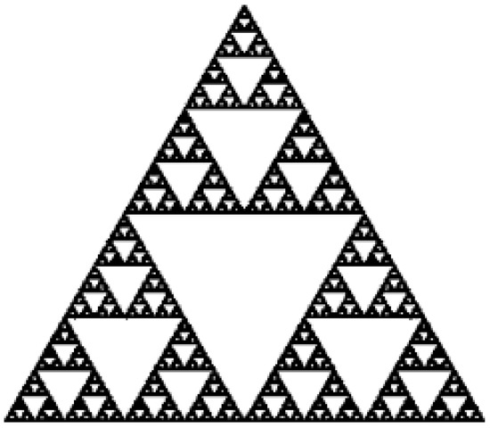 Figure 1. The Sierpinski triangle.
Conditions (CUCP1)–(CUCP3) assure coherence of the conditional upper previsions when the domain is a linear space of bounded random variables. In the sequel, we recall the properties of a conditional aggregation operator that allow for the construction a coherent upper conditional prevision by means of conditional aggregation operators.
We say that a conditional aggregation function A is sub-additive if and only if
holds for all . We say that a conditional aggregation function is positively homogeneous if and only if
for all and all .
In particular, a conditional aggregation function is idempotent if and only if
for all .
Lastly, we say that a conditional aggregation function is shift-invariant if and only if
for all and all .
A conditional aggregation function is linear if and only if it is shift-invariant and positively homogeneous.
Proposition 1.
A positively homogeneous conditional aggregation operator satisfies the following conditions:
- (a)
- is idempotent;
- (b)
- .
Proof.
(a) Because is positively homogeneous we have, by condition (2b) of Definition 1, that
for all .
(b)
□
Proposition 2.
Let be a sub-additive, positively homogeneous, and shift-invariant aggregation function such that . Then, the mapping given by
for all defines a coherent upper conditional prevision.
Proof.
By Proposition 3 of [14] we have that conditions (CUCP1)–(CUCP3) are satisfied. □
Coherent upper conditional probabilities can be obtained by Proposition 2 when only indicator functions are considered
Because , then the coherent upper conditional probability of an event E given B satisfies the following equality
For a coherent upper conditional probability, the following equalities hold:
The following example shows that there are conditional aggregation operators which cannot define coherent upper conditional previsions, but they can define a coherent upper conditional probability.
Example 5.
We can observe that the strongest conditional aggregation operator is a sub-additive but not positively homogeneous and shift-invariant aggregation operator on the class of all non-negative bounded random variables; so, it cannot be used to construct a coherent upper conditional prevision on the class of all random variables. Nevertheless, let then if and if and for all .
3. Composed Conditional Aggregation Operators
In this section, we investigate if composed aggregation operators are conditional aggregation operators. In that case, coherent upper conditional previsions are constructed by the composition of conditional aggregation operators according to Definition 1.
Theorem 1.
Let and let be a partition of Ω; for let be a positively homogeneous conditional aggregation and let be a class of conditional aggregation operators. Then, the composed conditional operator defined by
is a conditional aggregation operator.
Proof.
By condition (a) of Proposition 1 we have that any positively homogeneous conditional aggregation is idempotent, so the composed operator is an aggregation operator. Moreover, because are conditional aggregation operators we have that
and
so that conditions (2a) and (2b) of Definition 1 are satisfied and is a conditional aggregation operator. □
Remark 1.
According to Definition 1, a positive homogeneous conditional aggregation operator is idempotent, and it always defines a composed aggregation operator. If a conditional aggregation operator satisfies only one if the two conditions (2) of Definition 1, then the composed operator may be not a conditional aggregation operator.
Example 6.
Let X be a function such that for every , let , and let conditional aggregation operators defined by where each is a monotone set function such that . Then, the composed aggregation operator
is a composed conditional aggregation operator.
Because the Sugeno integral is not positively homogenous, the composed operator
is not a composed conditional aggregation operator.
Theorem 2.
Let, let, and letbe a class such thatare conditional aggregation operators which are sub-additive, positively homogeneous, and shift-invariant; then, the composed conditional operator defined onby
is a sub-additive, positively homogeneous, and shift-invariant conditional aggregation operator.
Proof.
For every we have
;
and
;
. ⋄□
By Theorem 2, the conditional aggregation operator defined in Example 5 is not sub-additive, positively homogeneous, and shift-invariant.
Given a metric space , let be a metric space such that is a bounded metric bi-Lipschitz equivalent to the metric d. Then, events which have a zero Hausdorff measure in a metric space also have a Hausdorff measure equal to zero in a metric space with a bi-Lipschitz equivalent metric.
Two different notions of equivalence can be considered for metrics: bi-Lipschitz equivalence [33] and topological equivalence.
Definition 3.
Letbe a metric space. A metricon Ω is bi-Lipschitz equivalent to the metric d if there exist two positive real constants such that
Definition 4.
Letbe a metric space and letbe a metric on Ω; d and are topological equivalent if they induce the same topology.
Proposition 3.
Letbe a metric space and letbe a metric on Ω bi-Lipschitz equivalent to d. Then, d and are topological equivalent.
The following example shows that the converse is not true.
Example 7.
is topological equivalent to the Euclidean metric d, as any open set inis an open set inand vice-versa because the topology τ induced by a metric d contains the empty set and the sets which are countable or finite unions of the. The metricis not bi-Lipschitz equivalent to d because there does not exist two positive real constantssuch thatas d is unbounded onwhile.
Letbe the Euclidean metric space and letbe a metric ondefinedby
In the following example, bi-Lipschitz equivalent distances are given.
Example 8.
Letand letdefined by
The distancesare bi-Lipschitz becausewe have
Theorem 3.
Letbe a metric space, let d andbe two metrics on Ω bi-Lipschitz equivalent and letandbe the s-dimensional Hausdorff measures defined, respectively, in the metric spaceand; then, there exists two positive real constantssuch that
Proof.
The result follows by the definition of Hausdorff outer measures and by the fact that the metrics are bi-Lipschitz equivalent (see Lemma 1.8 of [31]). □
Theorem 4.
Letbe a metric space and letbe a metric on Ω bi-Lipschitz equivalent to d. Then, the Hausdorff dimension of any set is invariant in the two metric spaces and .
The Hausdorff dimension of any set is not invariant with respect to two topological equivalent metrics which are not bi-Lipschitz equivalent.
Example 9.
which are sub-additive, positively homogeneous, and shift-invariant. Let be the composed aggregation operator
where the supremum is over ; then is sub-additive, positively homogeneous, shift-invariant, and by Theorem 2 we can construct a coherent upper conditional prevision by . The restriction to the to the class of all indicator functions of Borel sets of is a coherent conditional absolutely continuous with respect to all s-dimensional Hausdorff measures defined in metric spaces with metrics which are bi-Lipschitz equivalent.
Given a metric spaceand a partitionof Ω, let be a set with positive and finite Hausdorff outer measure in its dimension s, let be the class of all metrics on Ω which are bi-Lipschitz equivalent to d. Denote by the s-dimensional Hausdorff outer measures defined in with . Consider the following conditional aggregation operators
The following example shows that if all with do not satisfy condition (2b) of Definition 1 then the composed aggregation operator is not a conditional aggregation operator because it does not satisfy condition (2b) of Definition 1.
Example 10.
Letandand let m be the Lebesgue measure on the Borel sigma-field of Ω, the Choquet integral (which in this case coincides with the Lebesgue integral) is a conditional operator, but it does not define a conditional aggregation operator because it does not satisfy condition (2b) of Definition 1. Let and let A be a positively homogeneous conditional aggregation operator; then the composed operator is not a conditional aggregation operator because condition (2b) of Definition 1 is not satisfied
4. The Disintegration Property
Up to now, we have recalled the properties which assure that a conditional aggregation operator with respect to a conditioning event can be used to construct coherent upper conditional previsions. Now, the notion of a conditional aggregation operator with respect to a partition is introduced. This allows for the investigation of the coherence of the coherent upper conditional prevision with the unconditional upper prevision.
By Theorem 2 we have the following example of conditional aggregation operator
Example 11.
Letbe a partition of Ω and for each let be a positively homogenous conditional aggregation operator on . Then, the composed conditional operator
is a conditional aggregation operator.
Proposition 4.
If for everyis a sub-additive, positively homogeneous, and shift-invariant aggregation operator, then the operatoris an aggregation operator and it can define a coherent upper prevision.
Proof.
The result is a consequence of Theorem 2 when . □
Condition (2b) of Definition 1 assures that aggregating the random variable by a positively homogeneous conditional aggregation when the conditioning event B belongs to the partition of singletons is equivalent to knowing the random variable.
Proposition 5.
Let and let be a positively homogeneous conditional aggregation property. Then, for every we have .
Proof.
Denote . Then, by Proposition 1 and condition (2b) of Definition 1 we have so that . □
Remark 2.
Proposition 5 assures the intuitive result that aggregating a random variable X on the partition of singletons is equivalent to knowing the random variable itself. This property may be not satisfied if the conditional aggregation operator does not satisfy condition (2b) of Definition 1.
Definition 5.
A coherent upper conditional prevision satisfies the disintegration property with respect to the partition Bif and only if for all
If is a sub-additive, positively homogeneous, and shift-invariant aggregation operator, it can be used to construct a coherent upper conditional prevision and the disintegration property can be written in terms of conditional aggregation operators.
Example 12.
Ifis a finite set,a partition of Ω, and the conditional aggregation operator is the weighted average, the disintegration property is equivalent to
Example 13.
Let, letbe a Borel measurable partition of Ω, and let the conditional aggregation operator , that is, it is the Choquet integral with respect to the s-dimensional Hausdorff outer measure where s is the Hausdorff dimension of Ω. In [10,28], it is proven that the disintegration property holds and it is equivalent to
5. Conclusions
The notion of a conditional aggregation operator is important and useful when we want to aggregate data from different sources. In this paper, different sources are represented by atoms of a partition. In this framework, aggregating a function on the partition of singletons is equivalent to knowing the function. The definition of conditional aggregation operator given in this paper guarantees this intuitive property. A positively homogeneous conditional aggregation operator is proven to be always idempotent so that a composed operator is always a composed conditional aggregation operator. The findings proposed in this paper give sufficient conditions for a coherent upper conditional prevision to be defined by composed conditional aggregation operators. In particular, it is proven that a coherent conditional prevision can be obtained by the composed conditional aggregation operator which is the supremum of the class of coherent upper conditional previsions defined by the Choquet integrals with respect to the s-dimensional Hausdorff measures defined in metric spaces with metrics which are bi-Lipschitz. Conditional aggregation operators defined by Hausdorff outer measures can be applied in the continuous case, for instance when is an interval of and not in the finite case. In fact, if is a finite set, all of its subsets have Hausdorff dimensions equal to zero and the Choquet integral with respect to the 0-Hausdorff measure, which is the counting measure, is the weight average. A possible application of conditional aggregation operators based on Hausdorff outer measures is in management of big data that can be classified according their Hausdorff dimension or fractal dimension. A future work involves the consideration other conditional aggregation operators defined in a metric space by different dimensional measures, investigation of their properties, and consideration of these models for representing human brain activity and human decision making.
Funding
This research received no external funding.
Data Availability Statement
Not applicable.
Conflicts of Interest
The author declares no conflict of interest.
References
- Billingsley, P. Probability and Measure; Wiley: Hoboken, NJ, USA, 1986. [Google Scholar]
- De Finetti, B. Theory of Probability; Wiley: London, UK, 1974. [Google Scholar]
- Dubins, L.E. Finitely additive conditional probabilities, conglomerability and disintegrations. Ann. Probab. 1975, 3, 89–99. [Google Scholar] [CrossRef]
- Regazzini, E. Finitely additive conditional probabilities. Rend. Del Semin. Mat. Fis. Milano 1985, 55, 69–89. [Google Scholar] [CrossRef]
- Regazzini, E. De Finetti’s coherence and statistical inference. Ann. Stat. 1987, 15, 845–864. [Google Scholar] [CrossRef]
- Walley, P. Statistical Reasoning with Imprecise Probabilities; Chapman and Hall: London, UK, 1991. [Google Scholar]
- Doria, S. Characterization of a coherent upper conditional prevision as the Choquet integral with respect to its associated Hausdorff outer measure. Ann. Oper. Res. 2012, 195, 33–48. [Google Scholar] [CrossRef]
- Doria, S. Symmetric coherent upper conditional prevision by the Choquet integral with respect to Hausdorff outer measure. Ann. Oper. Res. 2014, 229, 377–396. [Google Scholar] [CrossRef]
- Doria, S. On the disintegration property of a coherent upper conditional prevision by the Choquet integral with respect to its associated Hausdorff outer measure. Ann. Oper. Res. 2017, 216, 253–269. [Google Scholar] [CrossRef]
- Doria, S.; Dutta, B.; Mesiar, R. Integral representation of coherent upper conditional prevision with respect to its associated Hausdorff outer measure: A comparison among the Choquet integral, the pan-integral and the concave integral. Int. J. Gen. Syst. 2018, 216, 569–592. [Google Scholar] [CrossRef]
- Doria, S. Preference orderings represented by coherent upper and lower previsions. Theory Decis. 2019, 87, 233–259. [Google Scholar] [CrossRef]
- Doria, S.; Mesiar, R.; Šeliga, A. Construction method of coherent lower and upper previsions based on collection integrals. Boll. dell’Unione Mat. Ital. 2020, 3, 469–476. [Google Scholar] [CrossRef]
- Doria, S.; Mesiar, R.; Šeliga, A. Integral representation of coherent lower previsions by super-additive integrals. Axioms 2020, 9, 43. [Google Scholar] [CrossRef]
- Doria, S.; Mesiar, R.; Šeliga, A. Sub-additive aggregation functions and their applications in construction of coherent upper previsions. Mathematics 2021, 9, 2. [Google Scholar] [CrossRef]
- Beliakov, G.; Pradera, A.; Calvo, T. Aggregation Functions: A Guide for Practitioners; Springer: Berlin/Heidelberg, Germany, 2007; ISBN 978-3-540-73720-9. [Google Scholar]
- Calvo, T.; Kolesarová, A.; Komorníková, M.; Mesiar, R. Aggregation operators: Properties, classes and construction methods. In Aggregation Operators; Physica: Heidelberg, Germany, 2002; pp. 3–104. [Google Scholar]
- Grabisch, M.; Marichal, J.L.; Mesiar, R.; Pap, E. Aggregation Functions; Cambridge University Press: Cambridge, UK, 2009. [Google Scholar]
- Torra, V.; Narukawa, Y. Modeling Decison: Information Fusion and Aggregation Operators; Springer: Berlin/Heidelberg, Germany, 2007. [Google Scholar]
- Greco, S.; Mesiar, R.; Rindone, F.; Šipeky, L. Superadditive and subadditive transformations of integrals and aggregation functions. Fuzzy Sets Syst. 2016, 291, 40–53. [Google Scholar] [CrossRef]
- Kouchakinejad, F.; Šipošová, A.; Širáň, J. Aggregation functions with given super-additive and sub-additive transformations. Int. J. Gen. Syst. 2017, 46, 225–234. [Google Scholar] [CrossRef]
- Šipošová, A. A note on the superadditive and the subadditive transformations of aggregation functions. Fuzzy Sets Syst. 2016, 299, 98–104. [Google Scholar] [CrossRef]
- Hriňáková, K.; Šeliga, A. Remarks on super-additive and sub-additive transformations of aggregation functions. Tatra Mt. Math. Publ. 2018, 72, 55–66. [Google Scholar] [CrossRef]
- Choquet, G. Theory of capacities. Ann. l’Institut Fourier 1954, 5, 131–295. [Google Scholar] [CrossRef]
- Denneberg, D. Non-Additive Measure and Integral; Kluwer Academic: Dordrecht, The Netherlands, 1994. [Google Scholar]
- Denneberg, D. Conditioning (Updating) non-additive measures. Ann. Oper. Res. 1994, 52, 21–42. [Google Scholar] [CrossRef]
- Klement, E.P.; Mesiar, R.; Pap, E. A universal integral as common frame for Choquet integral and Sugeno integral. IEEE Int. Trans. Fuzzy Syst. 2010, 355, 178–187. [Google Scholar] [CrossRef]
- Dubois, D.; Prade, H. Updating with belief functions, ordinal conditional functions and possibility measures. In Proceedings of the Sixth Annual Conference on Uncertainty in Artificial Intelligence, MIT, Cambridge, MA, USA, 27–29 July 1990. [Google Scholar]
- Doria, S. Disintegration property for coherent upper conditional previsions defined by Hausdorff outer measures for bounded and unbounded random variables. Int. J. Gen. Syst. 2021, 50, 262–280. [Google Scholar] [CrossRef]
- Doria, S. Probabilistic independence with respect to upper and lower conditional probabilities assigned by Hausdorff outer and inner measures. Int. J. Approx. Reason. 2007, 46, 617–635. [Google Scholar] [CrossRef]
- Bozczek, M.; Halčinová, L.; Hutník, O.; Kaluszka, M. Novel survivel functions based on conditional aggrgation operators. Inf. Sci. 2020, 580, 705–719. [Google Scholar] [CrossRef]
- Falconer, K.J. The Geometry of Fractal Sets; Cambridge University Press: Cambridge, UK, 1986. [Google Scholar]
- Rogers, C.A. Hausdorff Measures; Cambridge University Press: Cambridge, UK, 1970. [Google Scholar]
- Drutu, C.; Kapovich, M. Geometric Group Theory; Colloquium Publications, AMS: Providence, RI, USA, 2018. [Google Scholar]
Publisher’s Note: MDPI stays neutral with regard to jurisdictional claims in published maps and institutional affiliations. |
© 2022 by the author. Licensee MDPI, Basel, Switzerland. This article is an open access article distributed under the terms and conditions of the Creative Commons Attribution (CC BY) license (https://creativecommons.org/licenses/by/4.0/).