Fuzzy Extension of Crisp Metric by Means of Fuzzy Equivalence Relation

Abstract

We develop an alternative approach to the fuzzy metric concept, which we obtain by fuzzy extension of a crisp metric d on a set X by means of a fuzzy equivalence relation E on the set ${\mathrm{I}\mathrm{R}}^{+}$. We call it an E-d metric and study its properties and relations with “classical” fuzzy metrics. Our special interest is in the topologies and fuzzy topologies induced by E-d metrics.

1. Introduction

Since the inception of fuzzy sets by L.A. Zadeh in 1965 [1], many researchers have focused on incorporating “classic” mathematical concepts and theories into a fuzzy sets context. Among the first and the most successful fuzzy counterparts are fuzzy topologies, first introduced by C.L. Chang [2], and fuzzy algebraic structures—fuzzy groups and groupoids introduced by A. Rosenfeld [3]. Naturally, several researchers were challenged by the idea to also introduce a fuzzy counterpart of a metric space, especially since one could expect that fuzzy metrics will have important applications in studying real world problems. Notable contributions to the field of metrics were provided by I. Kramosil and J. Michalek [4], A. George and P. Veeramani [5], Z. Deng [6], and O. Kaleva and S. Seikkala [7] (note the differences between the initial prerequisites used by these authors).

In all the above-mentioned cases, first the abstract definitions of a fuzzy topological space, fuzzy group, fuzzy metric space, etc. were introduced and basics of the corresponding theories were laid. Only at the second stage were some constructions (e.g., functors) developed in order to view crisp objects (a topological space, a group, a metric space et al.) in the framework of their fuzzy counterparts and to study interrelations between the newly built categories of fuzzy structures and the classical ones. As examples, one can mention Lowen functor $\omega$ interpreting a topological space as a stratified fuzzy topological space, George and Veeramani construction of the standard fuzzy metric $M_d$ from a metric d, etc.

A different approach to obtaining a fuzzy version of a mathematical concept is undertaken by M. Ying in a series of papers [8,9] in the case of a topology. Ying fuzzifies the definition of a topology by making an analysis of topological axioms by means of the fuzzy logic tools. The obtained concept was given the name fuzzifying topology and at present is studied and used by many researchers.

Yet another approach to presenting a fuzzy version of a classical mathematical concept is to construct an extension using a fuzzy equivalence relation. This approach is realized for numbers (or points) and functions in [10,11,12], and studied further in [13].

In our paper, we undertake an approach to build a fuzzy version of a metric by constructing an extension of a metric by means of a fuzzy equivalence relation. Namely, the idea is to make a fuzzification of a crisp metric, initially defined on a set X, taking into account that the set ${\mathrm{I}\mathrm{R}}^{+}$ (the codomain of the metric) is equipped with a fuzzy equivalence E.

Fuzzy Extension of an Ordinary Metric vs. Classical Fuzzy Metrics

In the literature, most of the authors dealing with fuzzy metrics realize them in the context of axioms introduced in [5,14]. These axioms are a reformulation of those originally defined in [4]. In [4], the idea for defining a fuzzy metric comes from the assertion that the considered value of a crisp metric $d(x,y)$ (which should by fuzzified or approximated) is smaller than a prior-given real number $\lambda$. In other words, the statement $d(x,y)<\lambda$ is fuzzified. In our work, we fuzzify $d(x,y)=\lambda$, which is going to be useful when dealing with applications.

In our work, we study the fuzzy extension of crisp metrics and investigate their connections with classical fuzzy metrics. Thus, our fuzzification of metric concepts means that each crisp metric is also a fuzzy metric.

Therefore, we define a fuzzy metric as the degree by which the observed crisp distance between x and y ($d(x,y)$) is equal to the real number $\lambda$ in a fuzzy sense. Namely, we define a fuzzy metric as a membership function $M:X\times X\times [0,\infty )\to [0,1]$ satisfying $M(x,y,\lambda )=E\left(d\right(x,y),\lambda )$, where $d:X\times X\to [0,\infty )$ is a crisp metric that should be approximated or fuzzified, $\lambda$ is a real number that could be equal to the distance between x and y, and $E:{\mathrm{I}\mathrm{R}}^{+}\times {\mathrm{I}\mathrm{R}}^{+}\to [0,1]$ is a fuzzy equivalence relation. Moreover, in our approach, we start from the assertion that we need to fuzzify the statement $d(x,y)=\lambda$, where $\lambda$ is an a priori real number.

Furthermore, we study examples and properties, specifically topological, of the fuzzy metric induced by a fuzzy equivalence relation.

Nowadays, interest in the study of the topological properties of fuzzy metrics is growing, since this, in addition to the idea of a theoretical construction, leads to fixed point theorems and applications. On the topic of the topological properties of classical fuzzy metrics, we refer the reader to [14,15,16,17,18,19,20,21,22,23,24,25,26]. Fuzzy metrics are successfully used for solving image processing problems [27,28,29], but their potential is not fully realized. They can be used in particular for segmentation, spectralization and compression problems. Fuzzy metrics have also shown their potential in solving optimization problems [30].

Our paper is organized as follows. In Section 2, we recall the main notions and results used throughout our paper, namely regarding triangular norms, fuzzy relations, and classical fuzzy metrics. In Section 3, we realize the main purpose of our paper. Specifically, we construct a fuzzy metric from a classical one and call it an extensional fuzzy metric or an E-d metric. In Section 4, we study this metric’s topological issues. In Section 5, we study the relations between fuzzy metrics defined by Kramosil–Michalek and George–Veeramani and E-d metrics defined in our paper. In the last section, the Conclusion, we discuss some perspectives for continuation of this work.

2. Preliminaries

2.1. Triangular Norms

We start with the definition of a t-norm, which plays the crucial role in defining transitivity for fuzzy relations:

Definition 1 

([31]). A triangular norm (t-norm for short) is a binary operation T on the unit interval $[0,1]$, i.e., a function $T:{[0,1]}^2\to [0,1]$ such that for all $a,b,c\in [0,1]$ the following four axioms are satisfied:

• $T(a,b)=T(b,a)$ (commutativity);
• $T(a,T(b,c\left)\right)=T\left(T\right(a,b),c)$ (associativity);
• $T(a,b)\le T(a,c)$ whenever $b\le c$ (monotonicity);
• $T(a,1)=a$ (a boundary condition).

We list some common t-norms below:

• $T_M(a,b)=min(a,b)$ (minimum t-norm);
• $T_P(a,b)=a·b$ (product t-norm);
• $T_L(a,b)=max(a+b-1,0)$ (ukasiewicz t-norm);
• $T_H(a,b)=\left\{\begin{array}{cc}\frac{a·b}{a+b-a·b}\hfill & if{a}^2+b^2\ne 0\hfill \\ 0\hfill & otherwise\hfill \end{array}\right.$ (Hamacher t-norm).

A t-norm T is called Archimedean if and only if, for all pairs $(a,b)\in {(0,1)}^2$, there is $n\in \mathbb{N}$ such that $\underset{ntimes}{T(a,a,\dots ,a)}<b$.

Product and ukasiewicz t-norms are Archimedean while the minimum t-norm is not.

Here, we recall an important tool for constructing and studying t-norms involving only a one-argument real function (additive generator) and addition. Later, we use the same tool for constructing fuzzy equivalence.

Definition 2 

([31]). Let $f:[a,b]\to [c,d]$ be a monotone function, where $[a,b]$ and $[c,d]$ are closed subintervals of the extended real line $[-\infty ,\infty ]$. The pseudo-inverse $f^{(-1)}:[c,d]\to [a,b]$ of f is defined by:

$$f^{(-1)}\left(y\right)=\left\{\begin{array}{cc}sup\{x\in [a,b]\mid f(x)<y\}\hfill & \mathrm{if}f\left(a\right)<f\left(b\right),\hfill \\ sup\{x\in [a,b]\mid f(x)>y\}\hfill & \mathrm{if}f\left(a\right)>f\left(b\right),\hfill \\ a\hfill & \mathrm{if}f\left(a\right)=f\left(b\right).\hfill \end{array}\right.$$

In the particular case of a strictly decreasing function f, the pseudo-inverse is:

$$f^{(-1)}\left(y\right)=sup\{x\in [a,b]\mid f\left(x\right)>y\}.$$

Definition 3 

([31]). An additive generator $g:[0,1]\to [0,\infty ]$ of a t-norm T is a strictly decreasing function which is also right-semicontinuous at 0 and satisfies $g\left(1\right)=0$, such that for all $(a,b)\in {[0,1]}^2$ we have

$$g\left(a\right)+g\left(b\right)\in Ran\left(g\right)\cup \left[g\right(0),\infty ],$$

$$T(a,b)=g^{(-1)}(g\left(a\right)+g\left(b\right)).$$

where $Ran\left(g\right)$ is the range of g.

If a t-norm T has an additive generator g, it is uniquely determined up to a non-zero positive constant. Each t-norm with an additive generator is Archimedean.

2.2. Fuzzy Relations

We continue with an overview of basic definitions and results regarding fuzzy relations. L.A. Zadeh first introduced definitions of fuzzy order and fuzzy equivalence relations in 1971 ([32]) under the names of fuzzy ordering and fuzzy similarity relations. In our paper, we use results on fuzzy orders that were defined with respect to a fuzzy equivalence relation and studied in [33,34].

Definition 4. 

A fuzzy binary relation R on a set S is a mapping

$R:S\times S\to [0,1]$.

Definition 5 

(see e.g., [33]). A fuzzy binary relation E on a set S is called a fuzzy equivalence relation with respect to a t-norm T (or T-equivalence), if and only if the following three axioms are fulfilled for all $a,b,c\in S$:

1.

$E(a,a)=1$ reflexivity;

2.

$E(a,b)=E(b,a)$ symmetry;

3.

$T\left(E\right(a,b),E(b,c\left)\right)\le E(a,c)$ T-transitivity.

The following result shows how a fuzzy equivalence relation can be constructed by means of a pseudo-metric.

Theorem 1 

([33]). Let T be a continuous Archimedean t-norm with an additive generator g. For any pseudo-metric d, the mapping

$$E_d(a,b)=g^{(-1)}(min(d(a,b),g\left(0\right)))=g^{(-1)}\left(d(a,b)\right)$$

is a T-equivalence.

Example 1. 

Let us consider the set of real numbers $S=\mathbb{R}$ and the metric $d(a,b)=|a-b|$ on it. Taking into account that $g_L\left(x\right)=1-x$ is an additive generator of $T_L$ (ukasiewicz t-norm), $g_P\left(x\right)=-ln\left(x\right)$ is an additive generator of $T_P$ (product t-norm), and that $g_H\left(x\right)=\frac{1-x}{x}$ is an additive generator of $T_H$ (Hamacher t-norm), we obtain the following fuzzy equivalence relations:

$$E_L(a,b)=max(1-|a-b|,0);$$

$$E_P(a,b)=e^{-|a-b|};$$

$$E_H(a,b)=\frac{1}{1+|a-b|}.$$

Definition 6 

([34]). A fuzzy binary relation L on a set S is called fuzzy order relation with respect to a t-norm T and a T-equivalence E (or T-E-order), if and only if the following three axioms are fulfilled for all $a,b,c\in S:$

1.

$L(a,b)\ge E(a,b)$E-reflexivity;

2.

$T\left(L\right(a,b),L(b,c\left)\right)\le L(a,c)$ T-transitivity;

3.

$T\left(L\right(a,b),L(b,a\left)\right)\le E(a,b)$T-E-antisymmetry.

A fuzzy order relation L is called strongly linear if and only if for all $a,b\in S:$

$$max\left(L\right(a,b),L(b,a\left)\right)=1.$$

The following theorem states that strongly linear fuzzy order relations are uniquely characterized as fuzzifications of crisp linear orders. Preliminarily, let us recall the definition of compactibility:

Definition 7. 

Let ⪯ be a crisp order on S and let E be a fuzzy equivalence relation on S. E is called compatible with ⪯ if and only if the following implication holds for all $a,b,c\in S:$ $a⪯b⪯c\Rightarrow$$E(a,c)\le E(b,c)andE(a,c)\le E(a,b).$

Theorem 2. 

Let L be a binary fuzzy relation on S and let E be a T-equivalence on S. Then, the following two statements are equivalent:

1.

L is a strongly linear T-E-order on S;

2.

There exists a linear order ⪯ the relation E is compatible with, such that L can be represented as follows:

$$L(a,b)=\left\{\begin{array}{cc}1,\hfill & \mathrm{if}a⪯b\hfill \\ E(a,b),\hfill & \mathrm{otherwise}.\hfill \end{array}\right.$$

This theorem shows that, if we have a set S, a linear order ⪯ on it, and a T-equivalence on S that is compatible with ⪯, then we can build a fuzzy linear order L, as shown above.

In our paper, we will use a fuzzy equivalence relation on set $S=[0,\infty )$ (the interval $[0,\infty )$, which will be denoted by $\mathrm{I}{\mathrm{R}}^{+}$) and the linear order ≤. For simplicity of reading, the elements from the set $\mathrm{I}{\mathrm{R}}^{+}$ will be denoted by letters $a,b,c,d$, and the elements from set X will be denoted by $x,y,z$.

2.3. Fuzzy Metrics

First, we recall the concept of a fuzzy metric on a set X introduced by Kramosil and Michalek [4] and revised by Grabiec [14]. Here, we call it a KM-fuzzy metric.

Definition 8 

([4]). A KM-fuzzy metric on a set X is a mapping $M:X\times X\times [0,\infty )\to [0,1]$ satisfying the following axioms for all $x,y,z\in X$ and all $t,s\in [0,\infty )$:

(KM0)

$M(x,y,0)=0$;

(KM1)

$M(x,y,t)=1$ for all $t>0$ if and only if $x=y$;

(KM2)

$M(x,y,t)=M(y,x,t)$;

(KM3)

$M(x,z,t+s)\ge T\left(M\right(x,y,t),M(y,z,s\left)\right)$;

(KM4)

$M(x,y,-):(0,\infty )\to [0,1]$ is left-continuous.

In [5], George and Veeramani revised the original definition of a fuzzy metric given by Kramosil and Michalek as follows:

Definition 9 

([5]). A $GV$-fuzzy metric on a set X is a mapping $M:X\times X\times (0,\infty )\to (0,1]$ satisfying the following axioms for all $x,y,z\in X$ and all $t,s\in (0,\infty )$:

(GV0)

$M(x,y,t)>0$;

(GV1)

$M(x,y,t)=1$ if and only if $x=y$;

(GV2)

$M(x,y,t)=M(y,x,t)$;

(GV3)

$M(x,z,t+s)\ge T\left(M\right(x,y,t),M(y,z,s\left)\right)$;

(GV4)

$M(x,y,-):(0,\infty )\to [0,1]$ is continuous.

Definition 10. 

A GV-fuzzy metric M is said to be strong if M satisfies for all $x,y,z\in X$ and $t>0$ the following stronger version of the triangle inequality:

(GV3’)

$M(x,z,t)\ge T\left(M\right(x,y,t),M(y,z,t\left)\right)$.

George and Veeramani wrote that “$M(x,y,t)$ can be thought of the degree of nearness between x and y with respect to t” and introduced examples:

$M_P(x,y,t)=e^{-\frac{d(x,y)}{t}};$$M_H(x,y,t)=\frac{t}{t+d(x,y)}=\frac{1}{1+\frac{d(x,y)}{t}}$, which are now widely used in the literature. These examples demonstrate the degree of nearness between x and y with respect to t and we can say even more that these mappings are fuzzy equivalence relations for each level t. Indeed, $M_P(x,y,t)$ for a fixed level t is a fuzzy equivalence relation with respect to the product t-norm and $M_H(x,y,t)$ for a fixed level t is fuzzy equivalence relation with respect to the Hamacher t-norm (see Example 1). However, if we understand $M(x,y,t)$ as the degree of nearness between x and y at the level t, interpretations of axioms (KM3) and (GV3) are unclear. For the above-mentioned examples, we can also prove that they are strong fuzzy metrics; furthermore, the majority of fuzzy metrics examples used in the literature are also strong fuzzy metrics. We provide examples of fuzzy metrics that are not strong using our research.

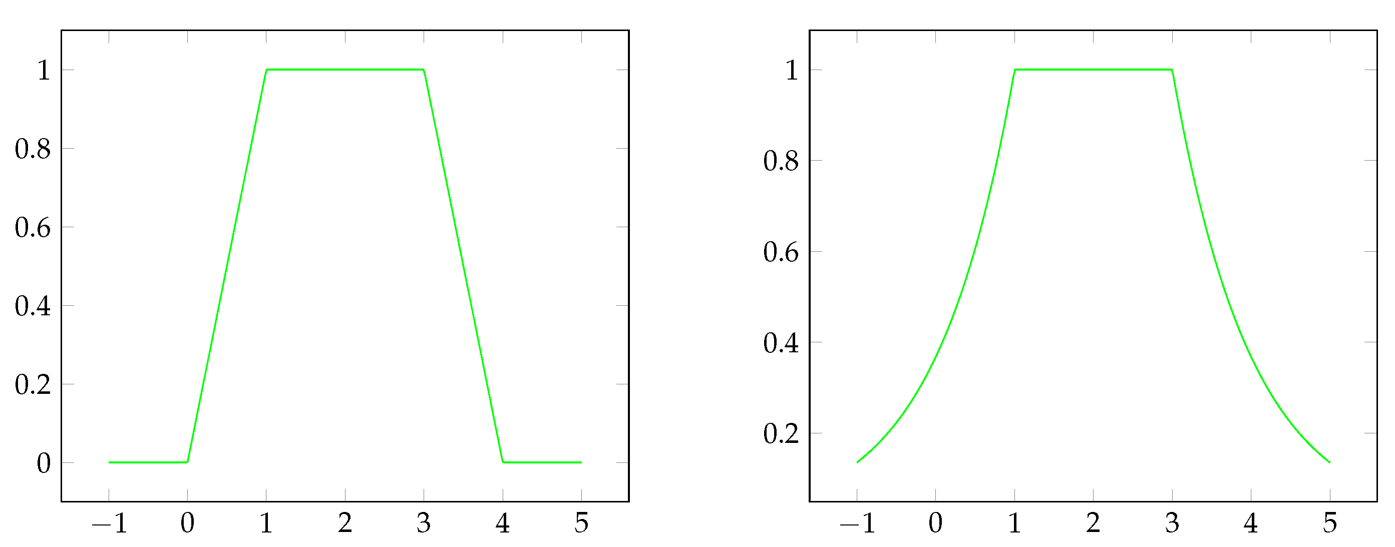
3. Fuzzy Equivalence Based Fuzzy Metrics

Consider a metric space $(X,d)$. We will define a fuzzy metric as an extension of the given metric d. We will extend the metric d with respect to a T-equivalence relation E on the set ${\mathrm{I}\mathrm{R}}^{+}$ (co-domain of the metric d). When defining the fuzzy metric, we will use a strongly linear T-E order on ${\mathrm{I}\mathrm{R}}^{+}$, defined as:

$$R_E(a,b)=\left\{\begin{array}{cc}1,\hfill & \mathrm{if}a\le b\hfill \\ E(a,b),\hfill & \mathrm{otherwise}\hfill \end{array}\right..$$

(1)

We propose to define fuzzy metric as the degree to which the observed distance $d(x,y)$ between points x and y is equal to the real number $\lambda$; equal in a certain fuzzy sense determined by fuzzy equivalence E. That is, we define a fuzzy metric (called E-d-metric) as a mapping $M_{Ed}:X\times X\times [0,\infty )\to [0,1]$:

Definition 11. 

Let d be a crisp metric on a set X, $t\in [0,\infty )$ and E be a fuzzy T-equivalence. Let a mapping $M_{Ed}:X\times X\times [0,\infty )\to [0,1]$ be defined as:

$$M_{Ed}(x,y,t)=E(d(x,y),t).$$

(2)

The fuzzy set $M_{Ed}$ is called an extensional fuzzy metric, which is determined by metric d and fuzzy equivalence E, or E-d-metric if the following condition is satisfied:

$$T(E(d(x,y),t),E(d(y,z),s))\le R_E(d(x,z),t+s).$$

(3)

The condition $T(E(d(x,y),t),E(d(y,z),s))\le R_E(d(x,z),t+s)$ shows that $d(x,y)=t$ and $d(y,z)=s$ implies $d(x,z)\le t+s$; implied in a certain fuzzy sense. In other words, it is a fuzzy version of triangular inequality. Note that fulfillment of the condition (3) depends both on the choice of metric d and equivalence relation E.

Remark 1. 

Note that the condition (3) is important for studying the topological issues of E-d-metric.

Remark 2. 

When defining the E-d-metric, T-equivalence relation E is defined on the set ${\mathrm{I}\mathrm{R}}^{+}\times {\mathrm{I}\mathrm{R}}^{+}$. Therefore, we use T-equivalence compatible with standard linear order ≤ on the real line $\mathrm{I}\mathrm{R}$.

Remark 3. 

If we have a crisp fuzzy equivalence relation,

$$E(a,b)=\left\{\begin{array}{cc}1,\hfill & \mathrm{if}a=b\hfill \\ 0,\hfill & \mathrm{otherwise},\hfill \end{array}\right.$$

then

$$R_E(a,b)=\left\{\begin{array}{cc}1,\hfill & \mathrm{if}a\le b\hfill \\ 0,\hfill & \mathrm{otherwise}.\hfill \end{array}\right.$$

Thus, for $M_{Ed}(x,y,t)=E(d(x,y),t)$, condition (3) holds for any t-norm T and metric d.

The next proposition states that if T is an Archimedean t-norm and a fuzzy equivalence relation on the set ${\mathrm{I}\mathrm{R}}^{+}$ is generated with respect to the distance $|a-b|$, where $a,b\in {\mathrm{I}\mathrm{R}}^{+}$, then the condition (3) is fulfilled for any metric $d:X\times X\to {\mathrm{I}\mathrm{R}}^{+}$.

Proposition 1. 

Let T be a continuous Archimedean t-norm with an additive generator g and T-equivalence be defined by:

$$E(a,b)=g^{(-1)}\left(\right|a-b\left|\right),$$

then the condition $T(E(d(x,y),t),E(d(y,z),s))\le R_E(d(x,z),t+s)$ is fulfilled for any metric d.

Proof. 

$T\left(E\right(d(x,y),t),E(d(y,z),s\left)\right)$$=T(g^{(-1)}\left(\right|d(x,y)-t\left|\right),g^{(-1)}\left(\right|d(y,z)-s\left|\right))=$

$g^{(-1)}\left(g\right(g^{(-1)}\left(\right|d(x,y)-t\left|\right))+g(g^{(-1)}\left(\right|d(y,z)-s\left|\right)\left)\right)=$$g^{(-1)}\left(\right|d(x,y)-t|+|d(y,z)-s\left|\right).$

Now consider two cases: when $d(x,z)\le t+s$ and when $d(x,z)>t+s$.

If $d(x,z)\le t+s$ then $T(E(d(x,y),t),E(d(y,z),s))\le R_E(d(x,z),t+s)$ since

$R_E(d(x,z),t+s)=1.$ If $d(x,z)>t+s$ then $R_E(d(x,z),t+s)=E(d(x,z),t+s)=$$g^{(-1)}\left(\right|d(x,z)-(t+s)\left|\right)=g^{(-1)}(d(x,z)-(t+s)).$

Now it is sufficient to prove that $\left|d\right(x,y)-t|+\left|d\right(y,z)-s|\ge d(x,z)-(t+s)$ if $d(x,z)>t+s$.

Let us consider four cases:

• If $d(x,y)>t$ and $d(y,z)>s$, then $\left|d\right(x,y)-t|+\left|d\right(y,z)-s|=d(x,y)-t+d(y,z)-s\ge d(x,z)-(t+s)$;
• If $d(x,y)\le t$ and $d(y,z)\le s$, then $d(x,z)\le d(x,y)+d(y,z)\le t+s$, which contradicts $d(x,z)>t+s$;
• If $d(x,y)\le t$ and $d(y,z)>s$, then $2d(x,y)\le 2t$ and $d(x,y)\le 2t-d(x,y)$. Hence, taking into account the latest, $d(x,z)\le d(x,y)+d(y,z)\le 2t-d(x,y)+d(y,z)$ and thus $d(x,z)-t-s\le t-d(x,y)+d(y,z)-s$, which means $\left|d\right(x,y)-t|+\left|d\right(y,z)-s|\ge d(x,z)-(t+s)$;
• If $d(x,y)>t$ and $d(y,z)\le s$, then the proof is similar to the previous case.

□

From this proposition, we obtain the following result, which is important for our work:

Theorem 3. 

Let T be a continuous Archimedean t-norm with an additive generator g and T-equivalence be defined by:

$$E(a,b)=g^{(-1)}\left(\right|a-b\left|\right),$$

then $M_{Ed}$ is an E-d-metric for any metric d.

Considering the previous theorem, we have the following examples:

Example 2. 

Let d be a crisp metric, $t\in [0,\infty )$. Then, we have the following examples of fuzzy metrics:

• $M_{E_{L}d}(x,y,t)=E_L(d(x,y),t)=max(1-|d(x,y)-t|,0)$ in case T is the ukasiewicz t-norm;
• $M_{E_{P}d}(x,y,t)=E_P(d(x,y),t)=e^{-\left|d\right(x,y)-t|}$ in case T is the product t-norm;
• $M_{E_{H}d}(x,y,t)=E_H(d(x,y),t)=\frac{1}{1+\left|d\right(x,y)-t|}$ in case T is the Hamaher t-norm.

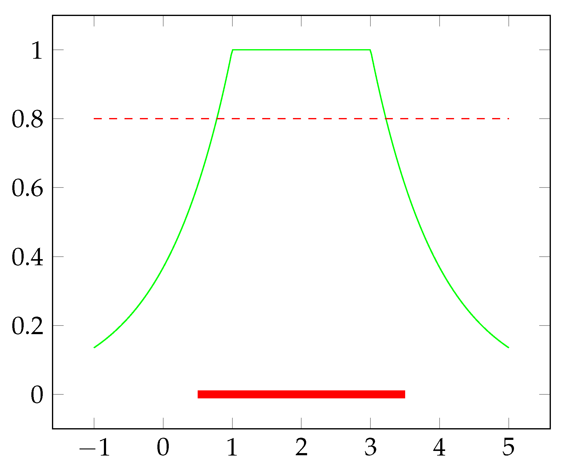
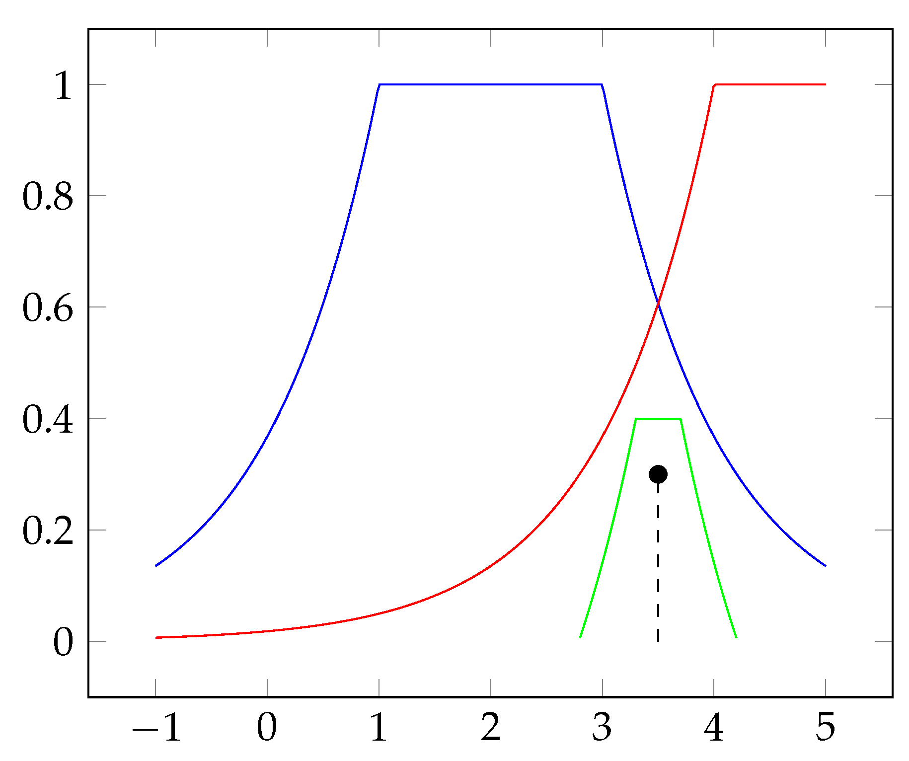
4. Topological Issues of E-d-Metrics

4.1. Topologies Generated by E-d-Metrics

In this section we study the topology induced by E-d-metrics. For topological issues, we additionally assume that the fuzzy equivalence $E:{\mathrm{I}\mathrm{R}}^{+}\times {\mathrm{I}\mathrm{R}}^{+}\to [0,1]$ is a lower-semicontinuous function. Given a metric d on a set x and a fuzzy equivalence $E:{\mathrm{I}\mathrm{R}}^{+}\times {\mathrm{I}\mathrm{R}}^{+}\to [0,1]$, we consider a fuzzy set ${\mathcal{B}}_{x,r}:X\to [0,1]$, where $x\in X$ and $r\in {\mathrm{I}\mathrm{R}}^{+}$, as follows:

$${\mathcal{B}}_{x,r}\left(y\right)=\left\{\begin{array}{cc}1,\hfill & \mathrm{if}d(x,y)<r\hfill \\ E\left(d\right(x,y),r),\hfill & \mathrm{otherwise}.\hfill \end{array}\right.$$

(4)

These fuzzy sets will play a significant role in our investigation and, thus, we visualize them in Figure 1.

Definition 12. 

For a given E-d-metric space $(X,M_{Ed})$, we define the ball $B(x,r,\alpha )$ with center $x\in X$, radius $r\in (0,\infty )$, and level $\alpha \in (0,1)$ as the strict α-cut of the fuzzy set ${\mathcal{B}}_{x,r}$ defined by formula (4).

Recall that a strict $\alpha$-cut of a fuzzy set $A:Y\to [0,1]$ is the set $\{y\in Y:A(y)>\alpha \}$.

Referring to formula (1), it is obvious that the above definition is equivalent to each one of the following two definitions:

Definition 13. 

For a given E-d-metric space $(X,M_{Ed})$, we define the ball $B(x,r,\alpha )$ with center $x\in X$, radius $r\in (0,\infty )$, and level $\alpha \in (0,1)$ as

$$B(x,r,\alpha )=\{y\in X:d(x,y)<r\}\cup \{y\in X:M_{Ed}(x,y,r)>\alpha \}.$$

Definition 14. 

For a given E-d-metric space $(X,M_{Ed})$, the ball $B(x,r,\alpha )$ with center $x\in X$, radius $r\in (0,\infty )$, and level $\alpha \in (0,1)$ is built as:

$$B(x,r,\alpha )=\{y\in X:R_E(d(x,y),r)>\alpha \}.$$

We visualize our obtained ball as the strict $\alpha$-cut of the fuzzy set ${\mathcal{B}}_{x,r}\left(y\right)$ by Figure 2.

Now we would like to demonstrate that a fuzzy set ${\mathcal{B}}_{x,r}$, defined by formula (4), is an extension of a crisp open ball from the metric space $(X,d)$ with center x and radius r by means of a fuzzy equivalence relation E. We recall that (see, e.g., Refs. [10,35]) a fuzzy set $A:Y\to [0,1]$ is called extensional with respect to a fuzzy equivalence relation E if $T\left(A\right(x),E(x,y\left)\right)\le A\left(y\right)$ for any $x,y\in Y$. If a fuzzy set is not extensional, it is possible to construct its extensional hull, which is the least extensional fuzzy set that contains the initial set. Naturally, an extensional hull of an extensional fuzzy set is the fuzzy set itself. The extensional hull of a fuzzy set $A:Y\to [0,1]$ may be constructed as follows: $EH\left(A\right)\left(x\right)={\bigvee }_{y\in Y}T(A\left(y\right),E(x,y)).$

It is easy to verify that if A is an interval $(a,b)\subset \mathrm{I}\mathrm{R}$ or a fuzzy set

$$A\left(x\right)=\left\{\begin{array}{cc}1,\hfill & \mathrm{if}a<x<b\hfill \\ 0,\hfill & \mathrm{otherwise},\hfill \end{array}\right.$$

then the extensional hull of the fuzzy set A is:

$$EH\left(A\right)\left(x\right)=\left\{\begin{array}{cc}1,\hfill & \mathrm{if}a\le x\le b\hfill \\ E(b,x),\hfill & \mathrm{if}x>b.\hfill \\ E(a,x),\hfill & \mathrm{if}x<a.\hfill \end{array}\right.$$

Let us observe an open ball $O(x,r)$ with a center x and radius r in a classical metric space $(X,d)$. Then, the extensional hull of $O(x,r)$, viewed as a fuzzy set, will be the fuzzy set ${\mathcal{B}}_{x,r}$ defined by formula (4).

Now we will prove that a ball $B(x,r,\alpha )$ is an open set in the following sense. Let us interpret a ball $B(x,r,\alpha )$ as a neighborhood of the point x. In the next proposition we show that a ball $B(x,r,\alpha )$ is an open set in the sense that each element of it is included in it together with a neighborhood; that is, for every $x_1\in B(x,r,\alpha )$ there exists a level $\beta$ and a radius $r_1$ such that $B(x_1,r_1,\beta )\subset B(x,r,\alpha )$. Therefore, we will call balls $B(x,r,\alpha )$ open balls.

Theorem 4. 

A ball $B(x,r,\alpha )$ is an open set.

Proof. 

Let us consider a ball

$$B(x,r,\alpha )=\{y\in X:d(x,y)<r\}\cup \{y\in X:M_{Ed}(x,y,r)>\alpha \},$$

and let $x_1\in B(x,r,\alpha )$. Then, we prove that there exists a level $\beta$ and radius $r_1$ such that:

$$B(x_1,r_1,\beta )\subset B(x,r,\alpha )$$

or, in other words, if $x_0\in B(x_1,r_1,\beta )$, then $x_0\in B(x,r,\alpha )$. Notice that $x_1\in B(x,r,\alpha )$ if and only if (by definition) $d(x,x_1)<r$ or $M_{Ed}(x,x_1,r)>\alpha$. Let us consider both cases:

• If $d(x,x_1)<r$, then for $r_1=r-d(x,x_1)$ and every $x_0\in B(x_1,r_1,\alpha )$, we also have two cases:

  (a)

  If $d(x_0,x_1)<r_1$, then $d(x_0,x)\le d(x_0,x_1)+d(x_1,x)<$$r-d(x,x_1)+d(x,x_1)=r$. This means $x_0\in B(x,r,\alpha )$;

  (b)

  If $d(x_0,x_1)\ge r_1$, then $M_{Ed}(x_0,x_1,r_1)>\alpha$ since $x_0\in B(x_1,r_1,\alpha )$. If $d(x,x_0)<r$, then obviously $x_0\in B(x,r,\alpha )$. Let us consider the case when $d(x,x_0)\ge r$; we are going to prove that $M_{Ed}(x,x_0,r)>\alpha$:

  $M_{Ed}(x,x_0,r)=E(d(x,x_0),r)=E(d(x,x_0),d(x,x_1)+r_1)$ because $r=d(x,x_1)+r_1$. Taking into account $d(x,x_0)\ge d(x,x_1)+r_1$ and condition (3) for E-d metric $M_{Ed}$, $M_{Ed}(x,x_0,r)=E(d(x,x_0),d(x,x_1)+r_1)=$ $R_E(d(x,x_0),d(x,x_1)+r_1)\ge$ $T(E(d(x,x_1,d(x,x_1)),E(d(x_1,x_0),r_1))=$ $T(1,E(d(x_1,x_0),r_1))=$

  $E(d(x_1,x_0),r_1)=M_{Ed}(x_0,x_1,r_1)>\alpha$. Note that, in this case, $\beta$ can be taken as $\alpha$.

• If $d(x,x_1)\ge r$ but $M_{Ed}(x,x_1,r)>\alpha$, then there exists $r^{\prime }<r$, such that $E(d(x,x_1),r^{\prime })>\alpha$ because E is lower-semicontinuous . Let $r_1=r-r^{\prime }$ and let us consider a point $x_0$.
  If $d(x,x_0)<r$, then obviously $x_0\in B(x,r,\alpha )$. Consider the case when $d(x,x_0)\ge r$; we are going to prove that a level $\beta$ exists such that, if $x_0\in B(x_1,r_1,\beta )$, then $x_0\in B(x,r,\alpha )$, which means $M_{Ed}(x,x_0,r)>\alpha$:
  $M_{Ed}(x,x_0,r)=E(d(x,x_0),r)=E(d(x,x_0),r^{\prime }+r_1)$ since $r=r^{\prime }+r_1$. Taking into account that $d(x,x_0)\ge r$, we conclude that $M_{Ed}(x,x_0,r)=E(d(x,x_0),r^{\prime }+r_1)=R_E(d(x,x_0),r^{\prime }+r_1)\ge$ $T(E(d(x,x_1),r^{\prime }),E(d(x_1,x_0),r_1))$.
  Further, there exists $\beta$ such that $T({\alpha }^{\prime },\beta )>\alpha$, where $E(d(x,x_1),r^{\prime })={\alpha }^{\prime }>\alpha$ and $M_{Ed}(x_1,x_0,r_1)>\beta$. Hence, $T(E(d(x,x_1),r^{\prime }),E(d(x_1,x_0),r_1))=T({\alpha }^{\prime },\beta )>\alpha$.

Thus the theorem is proved.

□

Remark 4. 

George and Veeramani [5] revised the definition of a KM-fuzzy metric to make studies of the induced topological structure more convenient. However, when George and Veeramani defined GV-fuzzy metrics, they not only formally changed the original definition but also indirectly changed the meaning of a fuzzy metric. Specifically, discussing open balls $B(x,t,r)=\{y:M(x,y,t)>1-r\}$, where x is the center and r is the radius, the radius is from the interval $[0,1]$ and t is interpreted as the level. Thus, according to this interpretation of a GV-fuzzy metric, the equality $M(x,y,t)=r$ characterizes the distance between points at level t, while in the case of KM-fuzzy metric value t in the equality, $M(x,y,t)=r$ describes the distance between points with the belief level r. In our investigations, the value $M_{Ed}(x,y,t)=r$ describes the belief level of the fact that the distance between points is t.

Proposition 2. 

For a given extensional fuzzy metric space $(X,M_{Ed})$ and an open ball $B(x,r,\alpha )$ in this space, where $x\in X,r\in (0,+\infty ),\alpha \in (0,1)$, there exists an $r^{\prime }\in (0,+\infty )$ such that open ball $O(x,r^{\prime })=\{y\in X:d(x,y)<r^{\prime }\}$ is equal to $B(x,r,\alpha )$, that is, $B(x,r,\alpha )=O(x,r^{\prime })$.

Proof. 

Let us consider a ball

$$B(x,r,\alpha )=\{y\in X:d(x,y)<r\}\cup \{y\in X:M_{Ed}(x,y,r)>\alpha \}.$$

Then, for

$$r^{\prime }=\underset{y\in B(x,r,\alpha )}{sup}d(x,y)$$

we have $B(x,r,\alpha )=O(x,r^{\prime })$:

If $x^{\prime }\in O(x,r^{\prime })$, then $d(x,x^{\prime })<{sup}_{y\in B(x,r,\alpha )}d(x,y)$ by the definition of $r^{\prime }$. Thus, $x^{\prime }\in B(x,r,\alpha )$.

If $x^{\prime }\in B(x,r,\alpha )$, then $d(x,x^{\prime })<{sup}_{y\in B(x,r,\alpha )}d(x,y)$ because $B(x,r,\alpha )$ is an open set. Thus, $x^{\prime }\in O(x,r^{\prime })$ by the definition of $r^{\prime }$ and $O(x,r^{\prime })$.

Thus the proposition is proved.

□

Taking into account Theorem 4 and Proposition 2, we have the following proposition:

Proposition 3. 

For a given metric space $(X,d)$ and an open ball $O(x,r)=\{y\in X:d(x,y)<r\}$ in this space, where $x\in X,r\in (0,+\infty )$, there exists $r^{\prime }\in (0,+\infty )$ and $\alpha \in (0,1)$ such that $O(x,r)=B(x,r^{\prime },\alpha )$.

Proposition 4. 

For a given E-d-metric space $(X,M_{Ed})$, the family

$$\left\{B\right(x,r,t):x\in X,r\in (0,+\infty ),t\in (0,1\left)\right\}$$

is a base of some topology ${\tau }_M$ on the set X. We call it the topology induced by the E-d-metric $M_{Ed}$.

Corollary 1. 

The family of open balls defined by E-d-metric $M_{E,d}$ coincides with the family of open balls defined by metric d. In particular, the topologies induced by $M_{Ed}$ and d coincide.

Corollary 2. 

The topology induced by E-d-metric is metrizable.

4.2. Fuzzy Topologies Generated by E-d-Metrics

In Proposition 2, we have proved that a ball $B(x,r,\alpha )=\{y\in X:d(x,y)<r\}\cup \{y\in X:M_{Ed}(x,y,r)>\alpha \}$ is an open ball in space $(X,d)$. However, in Theorem 4 we have proved something more, namely: for every $x_1\in B(x,r,\alpha )$ there exists a level $\beta$ and radius $r_1$ such that:

$$B(x_1,r_1,\beta )\subset B(x,r,\alpha ).$$

On the other hand, notice that:

$$r\le s⟹B(x,r,\alpha )\subset B(x,s,\alpha )and\alpha \le \delta ⟹B(x,r,\delta )\subset B(x,r,\alpha ).$$

The above statements say that we could adjust both level and radius to make a ball small enough.

It is also clear that dealing only with crisp topologies we could have for each level $\alpha$ the same set of open balls. So, we lose some information contained in the E-d-metric $M_{E,d}$ speaking only about crisp topologies. In order to take into account the separate role of a level and a radius we turn to the use of fuzzy topologies.

For the convenience of the reader, we recall basic concepts related to fuzzy topology.

4.2.1. Some Notions on Fuzzy Topologies

The first approach to the study of topological-type structures in the context of fuzzy sets was undertaken in 1968 by C.L. Chang [2]. According to this approach, a fuzzy topology on a set X is a subfamily of the family ${[0,1]}^X$ of fuzzy subsets of X satisfying certain counterparts of the usual topological axioms.

Definition 15 

([2]). A Chang fuzzy topology on X is a family $\tau \subseteq {[0,1]}^X$, that is, a subfamily of the family of fuzzy subsets of X, satisfying axioms:

1.

τ contains $0_X\left(x\right)=0\forall x\in X$ and $1_X\left(x\right)=1\forall x\in X$;

2.

τ is closed under finite meets, that is: $U\wedge V\in \tau$ for all $U,V\in \tau$;

3.

τ is closed under arbitrary joins, that is: ${\bigvee }_i{U}_i\in \tau$ for all $\{U_i:i\in I\}\subseteq {[0,1]}^X$.

Lowen, in [36], proposed to enrich Chang fuzzy topology with all constant fuzzy sets, thus the condition 1. is replaced by condition 1.*:

1.*$\tau$ contains all constant functions $c_X:X\to [0,1],$$c\in [0,1]$.

Here, we use this Lowen definition and, following [37], call such fuzzy topology stratified Chang fuzzy topology.

Definition 16 

([37]). Let $(X,\tau )$ be a fuzzy topology and ${\tau }_0\subseteq \tau$. ${\tau }_0$ is called a base of fuzzy topology τ if $\tau =\{\bigvee \mathcal{U}:\mathcal{U}\subseteq {\tau }_0\}$.

Definition 17 

([38]). A fuzzy point on X is a fuzzy set $x_a\in {[0,1]}^X$, where $x\in X$ and $\alpha \in (0,1)$ are defined as : $x_a\left(y\right)=\left\{\begin{array}{cc}a,\hfill & \mathrm{if}y=x\hfill \\ 0,\hfill & \mathrm{if}y\ne x.\hfill \end{array}\right.$

For a fuzzy set A and fuzzy point $x_a$, $x_a$ is said to be in A (in symbols $x_a\tilde{\in }A$) if $x_a\left(y\right)<A\left(y\right)$ for all $y\in suppA$, where $suppA=\{y\in X:A(y)>0\}$.

Theorem 5. 

Let ${\tau }_0$ be a family of fuzzy subsets of X. Then, ${\tau }_0$ is a base for some fuzzy topology τ if and only if the following two properties are satisfied.

1.

For every fuzzy point $x_a$ on X, there exists $B\in {\tau }_0$ such that $x_a\tilde{\in }B$;

2.

For every two $B_1,B_2\in {\tau }_0$ and every $x_a\tilde{\in }{B}_1\wedge B_2$ there exists $U\in {\tau }_0$ such that $x_a\tilde{\in }U\le B_1\wedge B_2$.

4.2.2. Fuzzy Topologies Generated by E-d-Metrics

In this subsection, we will construct fuzzy open balls, and thus fuzzy topology induced by an E-d-metric, taking into account all the prerequisites mentioned in the beginning of the section.

Defining a fuzzy topology induced by an E-d-metric, the first idea might be to use a family of fuzzy sets ${\mathcal{B}}_{x,r}:X\to [0,1]$ defined by formula (4) as the base for a fuzzy topology. Unfortunately it is not possible to prove that it is a base since, for arbitrary two open balls ${\mathcal{B}}_{x_1,r_1}$ and ${\mathcal{B}}_{x_2,r_2}$ and a fuzzy point $x_a$ from the intersection, we cannot always find a ball ${\mathcal{B}}_{x_3,r_3}$ such that $x_a\tilde{\in }{\mathcal{B}}_{x_3,r_3}\le {\mathcal{B}}_{x_1,r_1}\wedge {\mathcal{B}}_{x_2,r_2}$.

Figure 3 demonstrates the example, when for a point $x_a$ from the intersection of two open balls we could not find a ball which contains the point $x_a$ and is a subset of the intersection.

However, our aim is to obtain a base consisting of all open balls similarly as it is done in the classical case. To obtain a more flexible version of an open ball, we additionally introduce a level $\alpha \in (0,1]$ and built fuzzy open ball ${\mathcal{B}}_{x,r,\alpha }$ in order to obtain a topological base collecting open balls ${\mathcal{B}}_{x,r,\alpha }$ which will be used for a fuzzy topology we are going to construct.

The first idea would be to take intersections of a fuzzy set ${\mathcal{B}}_{x,r}$ and an arbitrary constant function. However, it does not work since we will not always be able to create a reconstruction of a fuzzy set

$${\mathcal{B}}_{x,r,\alpha }\left(y\right)=\left\{\begin{array}{cc}\alpha ,\hfill & \mathrm{if}d(x,y)<r\hfill \\ max\left\{E\right(d(x,y),r)-(1-\alpha ),0\},\hfill & \mathrm{otherwise},\hfill \end{array}\right.$$

until a fuzzy set

$${\mathcal{B}}_{x,r^{\prime }}\left(y\right)=\left\{\begin{array}{cc}1,\hfill & \mathrm{if}d(x,y)<r^{\prime }\hfill \\ E(d(x,y),r^{\prime }),\hfill & \mathrm{otherwise}.\hfill \end{array}\right.$$

Thus, the idea of constructing an open ball is in cutting a fuzzy set (4) by a constant function $f\left(y\right)=\alpha$, taking an upper part (which is $\ge \alpha$) and bringing it to the “bottom” by subtracting $\alpha$:

$${\mathcal{B}}_{x,r,\alpha }\left(y\right)=\left\{\begin{array}{cc}1-\alpha ,\hfill & \mathrm{if}d(x,y)<r\hfill \\ max\left\{E\right(d(x,y),r)-\alpha ,0\},\hfill & \mathrm{otherwise}.\hfill \end{array}\right.$$

(5)

Definition 18. 

The fuzzy set ${\mathcal{B}}_{x,r,\alpha }$ defined by (5) is called a fuzzy open ball with center x, radius r and level α.

Proposition 5. 

Family $\{{\mathcal{B}}_{x,r,\alpha }:x\in X,r\in [0,\infty ],\alpha \in [0,1]\}$ is a base of some fuzzy topology ${\tau }_{M_{Ed}}$.

Proof. 

It is clear that for each point we have a fuzzy open ball which contains this point. Now let $x_a\tilde{\in }{\mathcal{B}}_{x_1,r_1,{\alpha }_1}\wedge {\mathcal{B}}_{x_2,r_2,{\alpha }_2}$. This means $a<{\mathcal{B}}_{x_1,r_1,{\alpha }_1}\left(x\right)\wedge {\mathcal{B}}_{x_2,r_2,{\alpha }_2}\left(x\right)$. Further, the set $B_1=\{y\in X:{\mathcal{B}}_{x_1,r_1,{\alpha }_1}\left(y\right)>a\}$ which is the strict a-cut of the fuzzy set ${\mathcal{B}}_{x_1,r_1,{\alpha }_1}$ and the set $B_2=\{y\in X:{\mathcal{B}}_{x_2,r_2,{\alpha }_2}\left(y\right)>a\}$ which is the strict a-cut of the fuzzy set ${\mathcal{B}}_{x_2,r_2,{\alpha }_2}$ are the open balls in the metric space $(X,d)$, whose intersection is not an empty set (at least the point x belongs to this intersection). Thus, there exists an open ball with center x and a radius $r^{\prime }$, which belong to the intersection of the sets $B_1$ and $B_2$. Thus, by Proposition 2 there exist r and $a^{\prime }$ such that:

$${\mathcal{B}}_{x,r,a^{\prime }}\le {\mathcal{B}}_{x_1,r_1,{\alpha }_1}\wedge {\mathcal{B}}_{x_2,r_2,{\alpha }_2}.$$

□

5. Relations between Fuzzy Metrics and E-d-Metrics

In this section, we will show connections between fuzzy metrics defined by axioms (KM1)–(KM4) and their versions (GV1)–(GV4) on one side and E-d-metrics on the other side. However, taking into account that fuzzy metrics defined by axioms (KM1)–(KM4) and axioms (GV1)–(GV4) are increasing in the third argument and actually fuzzify the statement $d(x,y)<t$, we should modify E-d-metrics in the following way. Let us consider a mapping $M:X\times X\times [0,\infty )\to [0,1]$, defined as follows:

$$M(x,y,t)=\left\{\begin{array}{cc}1,\hfill & \mathrm{if}d(x,y)<t\hfill \\ M_{Ed}(x,y,t),\hfill & \mathrm{otherwise},\hfill \end{array}\right.$$

(6)

where d is a metric and E is a lower-continuous T-equivalence satisfying condition (3) and which separates points.

Here, we will show that a mapping $M:X\times X\times [0,\infty )\to [0,1]$, defined by (6), has properties closely related to the properties of fuzzy metrics defined by axioms (KM1)–(KM4) and axioms (GV1)–(GV4). Specifically, let us verify if a fuzzy set denoted by (6) satisfies axioms (KM1)–(KM4) and axioms (GV1)–(GV4):

• If $x=y$ then $d(x,y)=0$ and for each $t>0$$M(x,y,t)=1$.
  However, we could conclude that $x=y$ only if $M(x,y,t)=1$ for all $t>0$, which is equivalent to the (KM1) axiom;
• For sure, $M(x,y,t)=M(y,x,t)$ since metric d fulfils the symmetry condition, which is equivalent to (KM2) and (GV2) axioms;
• Let us prove that $T\left(M\right(x,y,t),M(y,z,s\left)\right)\le M(x,z,t+s)$, which is equivalent to (KM2) and (GV2) axioms:
  If $t+s>d(x,z)$ then $M(x,z,t+s)=1$ and condition
  $T\left(M\right(x,y,t),M(y,z,s\left)\right),\le M(x,z,t+s)$ fulfills immediately. Thus, we consider the case when $t+s\le d(x,z)$. Let us consider four cases:

  (a)

  If $t\le d(x,y)$ and $s\le d(y,z)$ then $T\left(M\right(x,y,t),M(y,z,s\left)\right)=$

  $=T\left(E\right(d(x,y),t),E(d(y,z),s\left)\right)\le M(x,z,t+s)$ because of the condition (1);

  (b)

  If $t>d(x,y)$ and $s>d(y,z)$ then $d(x,z)\le d(x,y)+d(y,z)<t+s$, which contradicts $t+s\le d(x,z)$, or in other words

  $T\left(M\right(x,y,t),M(y,z,s\left)\right)\le M(x,z,t+s)$ fulfills immediately;

  (c)

  If $t\le d(x,y)$ and $s>d(y,z)$ then $T\left(M\right(x,y,t),M(y,z,s\left)\right)=T\left(E\right(d(x,y),t),1)$ = $E\left(d\right(x,y),t)$. If $t\le d(x,y)$ and $s=d(y,z)$ then from the condition (3) we have

  $T\left(E\right(d(x,y),t),E(d(y,z),s\left)\right)=E\left(d\right(x,y),t)\le E\left(d\right(x,z),t+d(y,z\left)\right).$

  Now if $s>d(y,z)$ but still $t+s\le d(x,z)$ we have:

  $E\left(d\right(x,y),t)\le E\left(d\right(x,z),t+d(y,z\left)\right)\le E\left(d\right(x,z),t+s)$;

  (d)

  If $t>d(x,y)$ and $s\le d(y,z)$, then the proof is similar to the previous case.

• Continuity of M depends on continuity of E: if E is lower-semicontinuous then $M(x,y,-)$ is left-continuous; if E is continuous then $M(x,y,-)$ is continuous.

We finish by showing that (6) does not fulfill properties (KM0) and (GV0). First of all, $M(x,y,0)=1$ if $x=y$; that is why $M(x,y,0)\ne 0$ for all $x,y\in X$ and the axiom (KM0) is not fulfilled. The axiom (GV0) is also not fulfilled since $M(x,y,t)$ could take a value of 0 for a $t>0$. For example, if $E_L(a,b)=max(1-|a-b|,0)$ and $d(x,y)=|x-y|$, then $M(x,y,t)=0$ for all $x,y$ satisfying $d(x,y)>t>t-1$; for example, in this case, $M(2,4,1)=0$.

6. Conclusions

In this paper, we have introduced and studied the notion of an E-d-metric defined using a crisp metric and a fuzzy equivalence relation. In other words, it is a fuzzy extension of a crisp metric by means of a fuzzy equivalence relation. We can informally explain the difference between the Kramosil–Michalek metric and the E-d-metric by comparing metrics with fuzzy numbers. There are two different approaches to fuzzy numbers: Hutton numbers and triangular fuzzy numbers, or more precisely fuzzy extensional numbers. The former are used for topological constructions, the latter more for applications, and they fit the fuzzy extension principle.

We consider our research as providing a foundation for further defining the fuzzy metrics used in the literature by means of the fuzzy relations we applied for values of the crisp metrics $d(x,y)$ and t, which generalize the equality E we used in this study.

We are also interested in formulating axioms for a fuzzy metric without using a crisp metric d. However, we still want to fuzzify the statement $d(x,y)=\lambda$, where $\lambda$ is a prior-given real number. It would be interesting to study the connection of this defined fuzzy metric and an E-d-metric.

In the future, we will also study topologies where open balls are generated by taking strict $\alpha$-cuts of fuzzy sets $M_x\left(y\right)=E(x,y)$. In this case, the level could only be adjusted to be small enough for crisp balls. However, it remains to be seen if we can obtain the same topological spaces as for the E-d metric.

References

1. Zadeh, L.A. Fuzzy Sets. Inf. Control 1965, 8, 338–353. [Google Scholar] [CrossRef] [Green Version]
2. Chang, C.L. Fuzzy topological spaces. J. Math. Anal. Appl. 1968, 24, 182–190. [Google Scholar] [CrossRef] [Green Version]
3. Rosendeld, A. Fuzzy groups. J. Math. Anal. Appl. 1971, 35, 512–517. [Google Scholar] [CrossRef] [Green Version]
4. Kramosil, I.; Michalek, J. Fuzzy metrics and statistical metric spaces. Kybernetika 1975, 11, 336–344. [Google Scholar]
5. George, A.; Veeramani, P. On some results in fuzzy metric spaces. Fuzzy Sets Syst. 1994, 64, 395–399. [Google Scholar] [CrossRef] [Green Version]
6. Deng, Z. Fuzzy pseudo-metric spaces. J. Math. Anal. Appl. 1982, 86, 74–95. [Google Scholar] [CrossRef] [Green Version]
7. Kaleva, O.; Seikkala, S. On fuzzy metric spaces. Fuzzy Sets Syst. 1984, 12, 215–229. [Google Scholar] [CrossRef]
8. Ying, M. A new approach for fuzzy topology (I). Fuzzy Sets Syst. 1991, 39, 303–321. [Google Scholar] [CrossRef]
9. Ying, M. A new approach for fuzzy topology (II). Fuzzy Sets Syst. 1992, 47, 221–232. [Google Scholar] [CrossRef]
10. Klawonn, F.; Castro, J.L. Similarity in fuzzy reasoning. Mathw. Soft Comput. 1995, 2, 197–228. [Google Scholar]
11. Klawonn, F. Fuzzy points, fuzzy relations and fuzzy functions. In Discovering the World with Fuzzy Logic; Novak, V., Perfilieva, I., Eds.; Springer: Berlin/Heidelberg, Germany, 2000; pp. 431–453. [Google Scholar]
12. Klawonn, F.; Kruse, R. Equality relations as a basis for fuzzy control. Fuzzy Sets Syst. 1993, 54, 147–156. [Google Scholar] [CrossRef]
13. Holčapek, M.; Štěpnička, M. MI-algebras: A new framework for arithmetics of (extensional) fuzzy numbers. Fuzzy Sets Syst. 2014, 257, 102–131. [Google Scholar] [CrossRef]
14. Grabiec, M. Fixed points in fuzzy metric spaces. Fuzzy Sets Syst. 1988, 27, 385–389. [Google Scholar] [CrossRef]
15. George, A.; Veeramani, P. Some theorems in fuzzy metric spaces. J. Fuzzy Math. 1995, 3, 933–940. [Google Scholar]
16. George, A.; Veeramani, P. On some results of analysis for fuzzy metric spaces. Fuzzy Sets Syst. 1997, 90, 365–368. [Google Scholar] [CrossRef]
17. Gregori, V.; Miñana, J.-J. On fuzzy ψ-contractive sequences and fixed point theorems. Fuzzy Sets Syst. 2016, 300, 93–101. [Google Scholar] [CrossRef]
18. Gregori, V.; Miñana, J.-J.; Morillas, S.; Sapena, A. Cauchyness and convergence in fuzzy metric spaces. RACSAM 2017, 111, 25–37. [Google Scholar] [CrossRef]
19. Gregori, V.; Miñana, J.-J.; Morillas, S.; Sapena, A. On Principal Fuzzy Metric Spaces. Mathematics 2022, 10, 2860. [Google Scholar] [CrossRef]
20. Gregori, V.; Romaguera, S. Some properties of fuzzy metric spaces. Fuzzy Sets Syst. 2000, 115, 485–489. [Google Scholar] [CrossRef]
21. Gregori, V.; Romaguera, S. On completion of fuzzy metric spaces. Fuzzy Sets Syst. 2002, 130, 399–404. [Google Scholar] [CrossRef]
22. Gregori, V.; Romaguera, S. Characterizing completable fuzzy metric spaces. Fuzzy Sets Syst. 2004, 144, 411–420. [Google Scholar] [CrossRef]
23. Gregori, V.; Romaguera, S. Fuzzy quasi-metric-spaces. Appl. Gen. Topol. 2004, 5, 129–136. [Google Scholar] [CrossRef] [Green Version]
24. Gutiérrez-García, J.; Rodríguez-López, J.; Romaguera, S. On fuzzy uniformities induced by a fuzzy metric space. Fuzzy Sets Syst. 2018, 330, 52–78. [Google Scholar] [CrossRef]
25. Mihet, D. On fuzzy contractive mappings in Fuzzy metric spaces. J. Fuzzy Sets Syst. 2007, 158, 915–921. [Google Scholar] [CrossRef]
26. Romaguera, S.; Tirado, P. Characterizing complete fuzzy metric spaces via fixed point results. Mathematics 2020, 8, 273. [Google Scholar] [CrossRef] [Green Version]
27. Camarena, J.G.; Gregori, V.; Morillas, S.; Sapena, A. Fast detection and removal of impulsive noise using peer groups and fuzzy metrics. J. Vis. Commun. Image Represent. 2008, 19, 20–29. [Google Scholar] [CrossRef]
28. Morillas, S.; Gregori, V.; Peris-Fajarnés, G.; Latorre, P. A fast impulsive noise color image filtering using fuzzy metrics. Real-Time Imaging 2005, 11, 417–428. [Google Scholar] [CrossRef]
29. Morillas, S.; Gregori, V.; Peris-Fajarnés, G.; Sapena, A. Local self-adaptative fuzzy filter for impulsive noise removal in color image. Signal Process. 2008, 8, 330–398. [Google Scholar]
30. Grigorenko, O. Fuzzy Metrics for Solving MODM Problems. In Atlantis Studies in Uncertainty Modelling, Joint Proceedings of the 19th World Congress of the International Fuzzy Systems Association (IFSA), the 12th Conference of the European Society for Fuzzy Logic and Technology (EUSFLAT), and the 11th International Summer School on Aggregation Operators (AGOP), Bratislava, Slovakia, 19–24 September 2021. [Google Scholar]
31. Klement, E.P.; Mesiar, R.; Pap, E. Triangular Norms; Kluwer Academic Publishers: Dodrecht, The Netherlands, 2000. [Google Scholar]
32. Zadeh, L.A. Similarity relations and fuzzy orderings. Inform. Sci. 1971, 3, 177–200. [Google Scholar] [CrossRef]
33. De Baets, B.; Mesiar, R. Pseudo-metrics and T-quivalences. J. Fuzzy Math. 1997, 5, 471–481. [Google Scholar]
34. Bodenhofer, U. A similarity-based generalization of fuzzy orderings preserving the classical axioms. Internat. J. Uncertain. Fuzziness-Knowl.-Based Syst. 2000, 8, 593–610. [Google Scholar] [CrossRef] [Green Version]
35. Höhle, U. M-valued sets and sheaves over integral commutative clmonoids. In Applications of Category Theory to Fuzzy Subsets; Rodabaugh, S.E., Klement, E.P., Höhle, U., Eds.; Kluwer: Dodrecht, The Netherlands; Boston, MA, USA, 1992; pp. 33–72. [Google Scholar]
36. Lowen, R. Fuzzy topological spaces and fuzzy compactness. J. Math. Anal Appl. 1976, 56, 621–633. [Google Scholar] [CrossRef] [Green Version]
37. Liu, Y.-M.; Luo, M.-K. Fuzzy Topology; World Scientific: Singapore, 1997. [Google Scholar]
38. Wong, C.K. Fuzzy points and local properties of fuzzy topology. J. Math. Anal. Appl. 1974, 46, 316–328. [Google Scholar] [CrossRef]
Figure 1. A figure demonstrates the fuzzy sets B x , r ( y ) , where X = I R , x = 2 , r = 1 , d ( x , y ) = | x y | , E is the fuzzy equivalence relation with respect to the ukasiewicz t-norm (on the left) and product t-norm (on the right).
Mathematics 10 04648 g001
Figure 2. A figure demonstrates the ball obtained as the strict 0.8 -cut of the fuzzy set B 2 , 1 ( y ) , where d ( x , y ) = | x y | . X = I R , E is the fuzzy equivalence relation with respect to the product t-norm.
Mathematics 10 04648 g002
Figure 3. A figure demonstrates that for two fuzzy sets B 2 , 1 and B 5 , 1 and a point x a , where x = 3.5 and a = 0.3 , from the intersection, we cannot find a ball B x 3 , r 3 such that x a ˜ B x 3 , r 3 B 2 , 1 B 5 , 1 . X = I R , E is the fuzzy equivalence relation with respect to the product t-norm.
Mathematics 10 04648 g003
Publisher’s Note: MDPI stays neutral with regard to jurisdictional claims in published maps and institutional affiliations.