

Artificial Intelligence-Based Prediction of Crude Oil Prices Using Multiple Features under the Effect of Russia–Ukraine War and COVID-19 Pandemic


Abstract
1. Introduction
2. Material and Methods
2.1. Artificial Intelligence Methods
2.2. Performance Metrics
2.3. Dataset
2.4. The Proposed Method
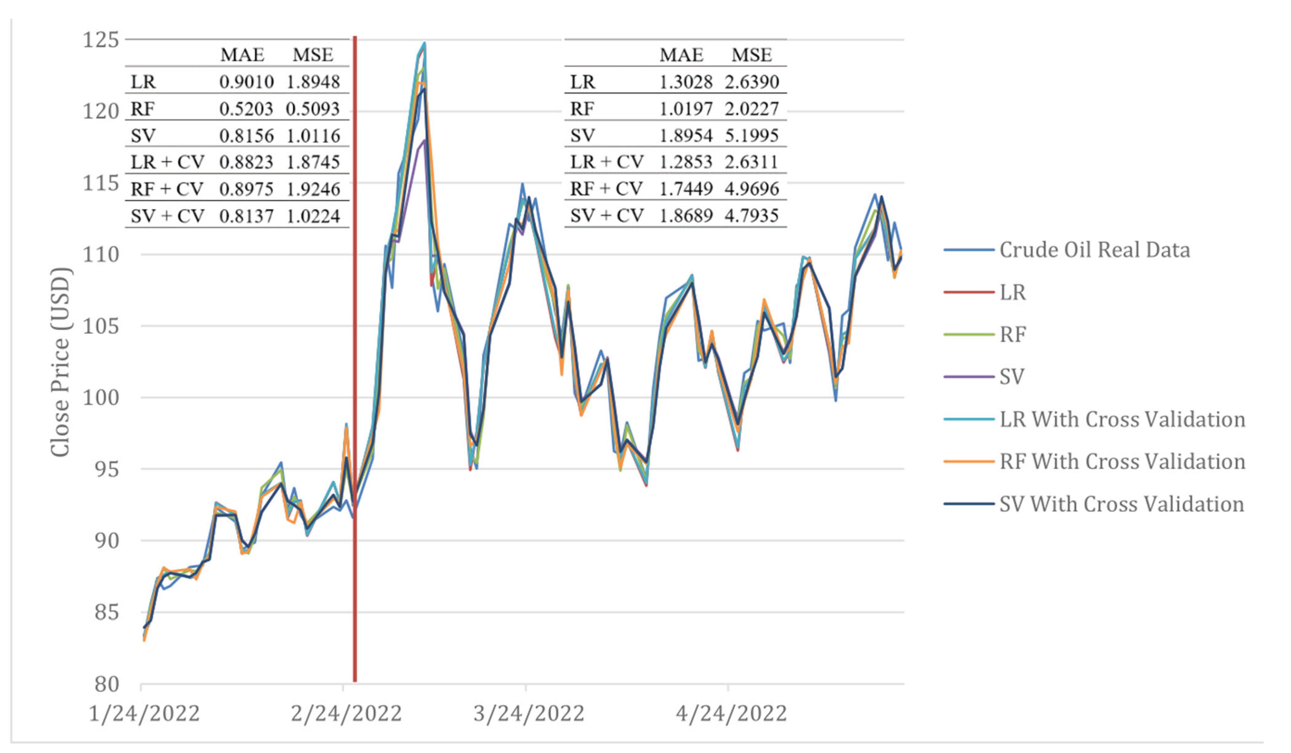
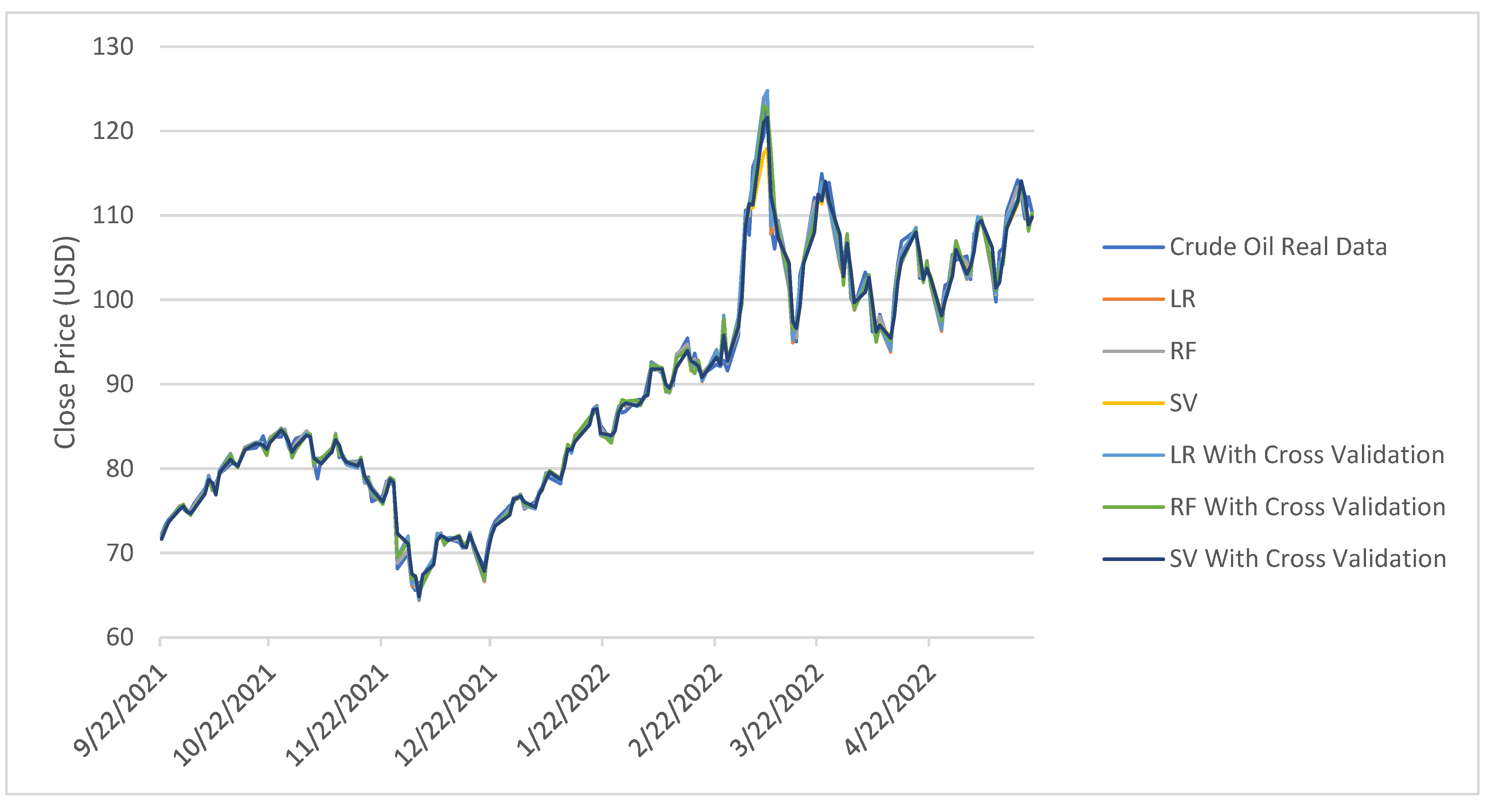
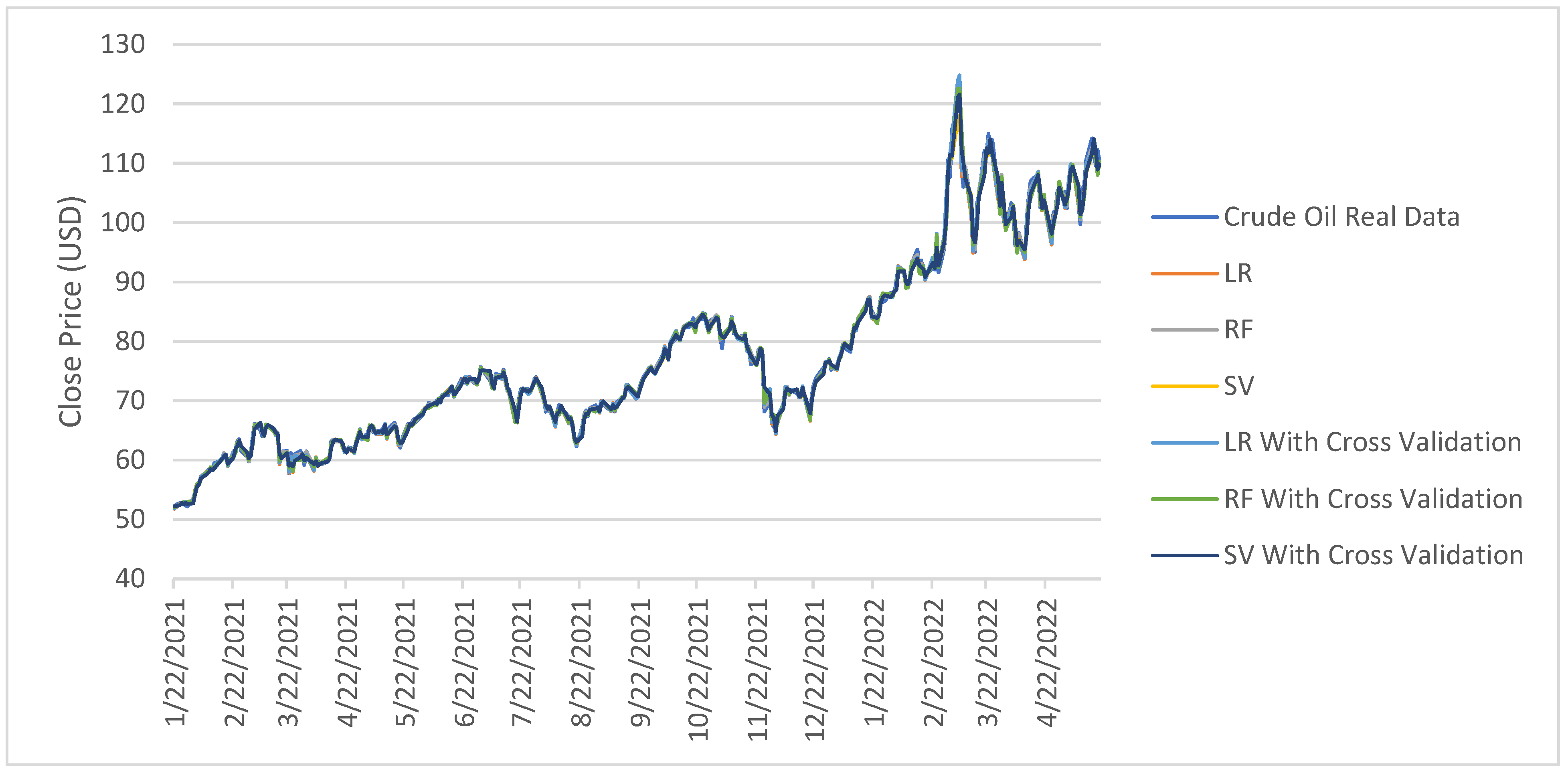
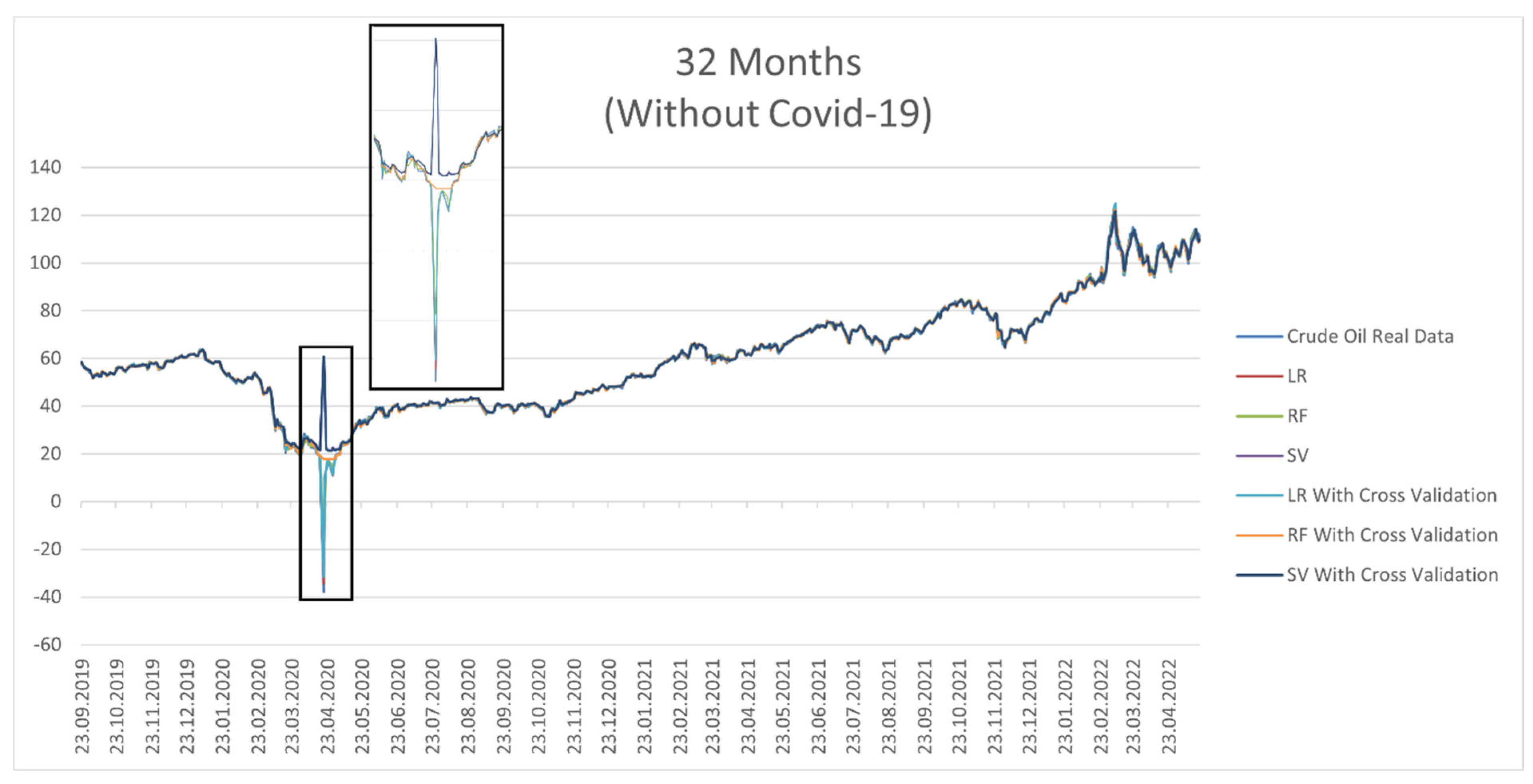
3. Experimental Results
4. Conclusions
Author Contributions
Funding
Data Availability Statement
Acknowledgments
Conflicts of Interest
References
- Deng, C.; Ma, L.; Zeng, T. Crude Oil Price Forecast Based on Deep Transfer Learning: Shanghai Crude Oil as an Example. Sustainability 2021, 13, 13770. [Google Scholar] [CrossRef]
- Sabah, N.; Sagheer, A.; Dawood, O. Blockchain-based solution for COVID-19 and smart contract healthcare certification. Iraqi J. Comput. Sci. Math. 2021, 2, 1–8. [Google Scholar] [CrossRef]
- Aggarwal, K.; Mijwil, M.M.; Sonia; Al-Mistarehi, A.-H.; Alomari, S.; Gök, M.; Alaabdin, A.M.Z.; Abdulrhman, S.H. Has the future started? The current growth of artificial intelligence, machine learning, and deep learning. Iraqi J. Comput. Sci. Math. 2022, 3, 115–123. [Google Scholar]
- Vo, A.H.; Nguyen, T.; Le, T. Brent oil price prediction using Bi-LSTM network. Intell. Autom. Soft Comput. 2020, 26, 1307–1317. [Google Scholar] [CrossRef]
- Gabralla, L.A.; Jammazi, R.; Abraham, A. Oil Price Prediction Using Ensemble Machine Learning. Proceeding of the International Conference on Computing, Electrical and Electronic Engineering (ICCEEE), Khartoum, Sudan, 26–28 August 2013; pp. 674–679. [Google Scholar]
- Kaymak, Ö.Ö.; Kaymak, Y. Prediction of crude oil prices in COVID-19 outbreak using real data. Chaos Solitons Fractals 2022, 158, 111990. [Google Scholar] [CrossRef]
- Karasu, S.; Altan, A. Crude oil time series prediction model based on LSTM network with chaotic Henry gas solubility optimization. Energy 2022, 242, 122964. [Google Scholar] [CrossRef]
- Gupta, N.; Nigam, S. Crude oil price prediction using artificial neural network. Procedia Comput. Sci. 2020, 170, 642–647. [Google Scholar] [CrossRef]
- Busari, G.A.; Lim, D.H. Crude oil price prediction: A comparison between AdaBoost-LSTM and AdaBoost-GRU for improving forecasting performance. Comput. Chem. Eng. 2021, 155, 107513. [Google Scholar] [CrossRef]
- Yao, L.; Pu, Y.; Qiu, B. Prediction of Oil Price Using LSTM and Prophet. Proceeding of the International Conference on Applied Energy, Bangkok, Thailand, 29 November–2 December 2021. [Google Scholar]
- Mukhamediev, R.I.; Popova, Y.; Kuchin, Y.; Zaitseva, E.; Kalimoldayev, A.; Symagulov, A.; Levashenko, V.; Abdoldina, F.; Gopejenko, V.; Yakunin, K.; et al. Review of Artificial Intelligence and Machine Learning Technologies: Classification, Restrictions, Opportunities and Challenges. Mathematics 2022, 10, 2552. [Google Scholar] [CrossRef]
- Ezugwu, A.E.; Ikotun, A.M.; Oyelade, O.O.; Abualigah, L.; Agushaka, J.O.; Eke, I.C.; Akinyelu, A.A. A comprehensive survey of clustering algorithms: State-of-the-art machine learning applications, taxonomy, challenges, and future research prospects. Eng. Appl. Artif. Intell. 2022, 110, 104743. [Google Scholar] [CrossRef]
- Nassif, A.B.; Talib, M.A.; Nasir, Q.; Afadar, Y.; Elgendy, O. Breast cancer detection using artificial intelligence techniques: A systematic literature review. Artif. Intell. Med. 2022, 110, 102276. [Google Scholar] [CrossRef] [PubMed]
- Wang, C.-N.; Yang, F.-C.; Nguyen, V.T.T.; Vo, N.T.M. CFD Analysis and Optimum Design for a Centrifugal Pump Using an Effectively Artificial Intelligent Algorithm. Micromachines 2022, 13, 1208. [Google Scholar] [CrossRef] [PubMed]
- Dhakal, A.; McKay, C.; Tanner, J.J.; Cheng, J. Artificial intelligence in the prediction of protein–ligand interactions: Recent advances and future directions. Brief. Bioinform. 2022, 23, bbab476. [Google Scholar] [CrossRef] [PubMed]
- Nguyen, T.V.T.; Huynh, N.T.; Vu, N.C.; Kieu, V.N.D.; Huang, S.C. Optimizing compliant gripper mechanism design by employing an effective bi-algorithm: Fuzzy logic and AN-FIS. Microsyst. Technol. 2021, 27, 3389–3412. [Google Scholar] [CrossRef]
- Kabeya, Y.; Okubo, M.; Yonezawa, S.; Nakano, H.; Inoue, M.; Ogasawara, M.; Saito, Y.; Tanboon, J.; Indrawati, L.A.; Kumutpongpanich, T.; et al. Deep convolutional neural network-based algorithm for muscle biopsy diagnosis. Lab. Investig. 2022, 102, 220–226. [Google Scholar] [CrossRef]
- Yuan, J.; Zhao, M.; Esmaeili-Falak, M. A comparative study on predicting the rapid chloride permeability of self-compacting concrete using meta-heuristic algorithm and artificial intelligence techniques. Struct. Concr. 2022, 23, 753–774. [Google Scholar] [CrossRef]
- Ismail, L.; Materwala, H.; Tayefi, M.; Ngo, P.; Karduck, A.P. Type 2 Diabetes with Artificial Intelligence Machine Learning: Methods and Evaluation. Arch. Comput. Methods Eng. 2022, 29, 313–333. [Google Scholar] [CrossRef]
- Sujith, A.V.L.N.; Sajja, G.S.; Mahalakshmi, V.; Nuhmani, S.; Prasanalakshmi, B. Systematic review of smart health monitoring using deep learning and Artificial intelligence. Neurosci. Inform. 2022, 2, 100028. [Google Scholar] [CrossRef]
- Cortes, V.; Cortes, C.; Vapnik, V. Support-vector networks. Mach. Learn. 1995, 20, 273–297. [Google Scholar] [CrossRef]
- Petridis, K.; Tampakoudis, I.; Drogalas, G.; Kiosses, N. A Support Vector Machine model for classification of efficiency: An application to M&A. Res. Int. Bus. Financ. 2022, 61, 101633. [Google Scholar]
- Gupta, I.; Mittal, H.; Rikhari, D.; Singh, A.K. MLRM: A Multiple Linear Regression based Model for Average Temperature Prediction of A Day. arXiv 2022, preprint. arXiv:2203.05835. [Google Scholar]
- Azar, A.T.; Elshazly, H.I.; Hassanien, A.E.; Elkorany, A.M. A random forest classifier for lymph diseases. Comput. Methods Programs Biomed. 2014, 113, 465–473. [Google Scholar] [CrossRef] [PubMed]
- Breiman, L. Random forests. Mach. Learn. 2001, 45, 5–32. [Google Scholar] [CrossRef]
- Amit, Y.; Geman, D. Shape quantization and recognition with randomized trees. Neural Comput. 1997, 9, 1545–1588. [Google Scholar] [CrossRef]
- Ho, T.K. Random decision forests. In Proceedings of the 3rd International Conference on Document Analysis and Recognition, Montreal, QC, Canada, 14–16 August 1995. [Google Scholar]
- Pal, M. Random forest classifier for remote sensing classification. Int. J. Remote Sens. 2005, 26, 217–222. [Google Scholar] [CrossRef]
- Belgiu, M.; Drăguţ, L. Random forest in remote sensing: A review of applications and future directions. ISPRS J. Photogramm. Remote Sens. 2016, 114, 24–31. [Google Scholar] [CrossRef]
- Cheng, J.; Kuang, H.; Zhao, Q.; Wang, Y.; Xu, L.; Liu, J.; Wang, J. DWT-CV: Dense weight transfer-based cross validation strategy for model selection in biomedical data analysis. Future Gener. Comput. Syst. 2022, 135, 20–29. [Google Scholar] [CrossRef]
- Smagulova, K.; James, A.P. A survey on LSTM memristive neural network architectures and applications. Eur. Phys. J. Spec. Top. 2019, 228, 2313–2324. [Google Scholar] [CrossRef]
- Khullar, S.; Singh, N. Water quality assessment of a river using deep learning Bi-LSTM methodology: Forecasting and validation. Environ. Sci. Pollut. Res. 2022, 29, 12875–12889. [Google Scholar] [CrossRef]
- Graves, A.; Fernández, S.; Schmidhuber, J. Bidirectional LSTM networks for improved phoneme classification and recognition. In International conference on artificial neural networks; Springer: Berlin/Heidelberg, Germany, 2005; Volume 3697, pp. 799–804. [Google Scholar]
- Shaik, N.B.; Pedapati, S.R.; Othman, A.R.; Bingi, K.; Dzubir, F.A.A. An intelligent model to predict the life condition of crude oil pipelines using artificial neural networks. Neural Comput. Appl. 2021, 33, 14771–14792. [Google Scholar] [CrossRef]
- Crude Oil Jul 22 (CL=F) Stock Historical Prices & Data—Yahoo Finance. Available online: https://finance.yahoo.com/quote/CL%3DF/history?p=CL%3DF (accessed on 3 June 2022).


| Layer Name | Used Layer | Layer Input | Layer Output |
|---|---|---|---|
| Input | Input Layer | [(None, 5507, 4)] | [(None, 5507, 4)] |
| Lstm_1 | LSTM | [(None, 5507, 4)] | [(None, 5507, 64)] |
| Lstm_2 | LSTM | [(None, 5507, 64)] | [(None, 5507, 128)] |
| dropout | Dropout | [(None, 128)] | [(None, 128)] |
| dense_1 | Dense | [(None, 128)] | [(None, 512)] |
| dense_2 | Dense | [(None, 512)] | [(None, 42)] |
| Layer Name | Used Layer | Layer Input | Layer Output |
|---|---|---|---|
| Input | Input Layer | [(None, 5507, 4)] | [(None, 5507, 4)] |
| Bidirectional_1 (lstm) | Bidirectional (LSTM) | [(None, 5507, 4)] | [(None, 5507, 64)] |
| Bidirectional_2 (lstm) | Bidirectional (LSTM) | [(None, 5507, 64)] | [(None, 5507, 128)] |
| dropout | Dropout | [(None, 128)] | [(None, 128)] |
| dense_1 | Dense | [(None, 128)] | [(None, 512)] |
| dense_2 | Dense | [(None, 512)] | [(None, 42)] |
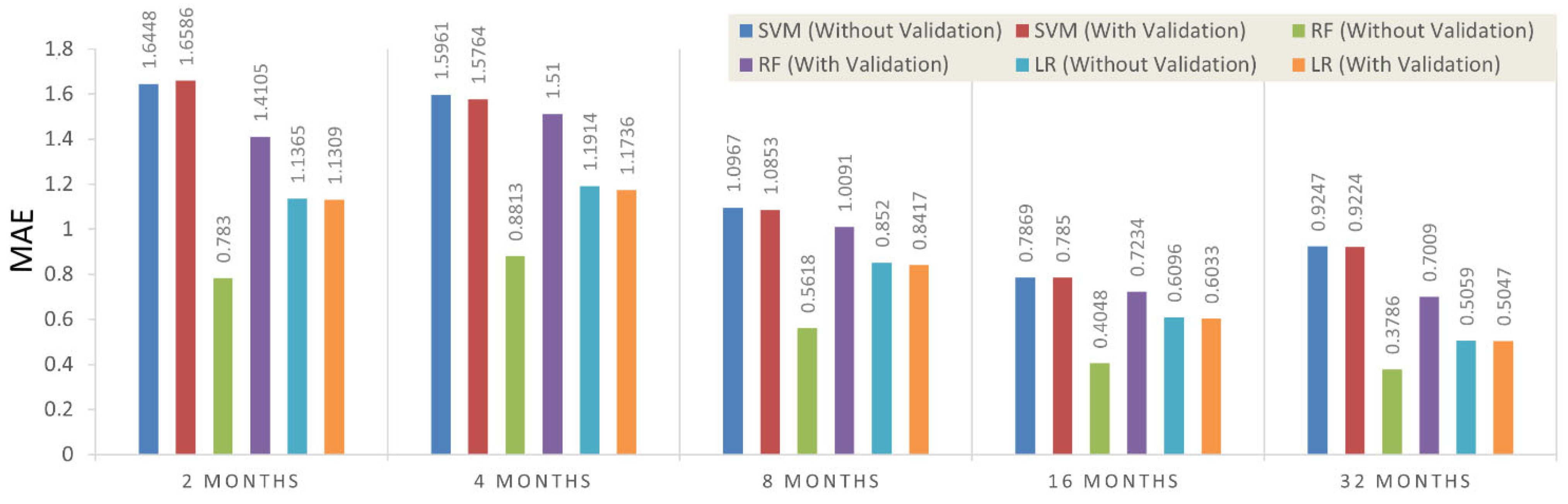
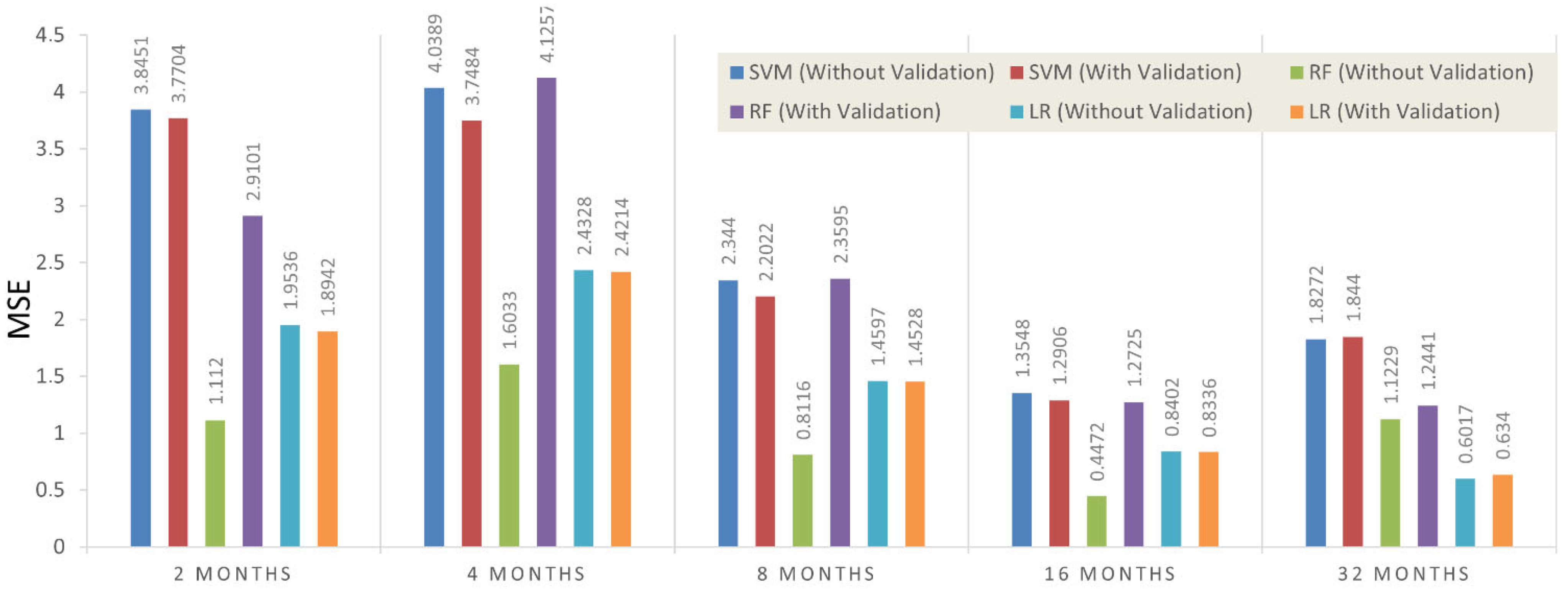
| Period | Performance Metrics | SVM | RF | LR | |||
|---|---|---|---|---|---|---|---|
| Without Validation | With Validation | Without Validation | With Validation | Without Validation | With Validation | ||
| Two months (without war) | MAE | 1.6448 | 1.6586 | 0.7830 | 1.4105 | 1.1365 | 1.1309 |
| MSE | 3.8451 | 3.7704 | 1.1120 | 2.9101 | 1.9536 | 1.8942 | |
| Four months (low COVID-19 effect) | MAE | 1.5961 | 1.5764 | 0.8813 | 1.5100 | 1.1914 | 1.1736 |
| MSE | 4.0389 | 3.7484 | 1.6033 | 4.1257 | 2.4328 | 2.4214 | |
| Eight months (two-year COVID-19 effect) | MAE | 1.0967 | 1.0853 | 0.5618 | 1.0091 | 0.8520 | 0.8417 |
| MSE | 2.3440 | 2.2022 | 0.8116 | 2.3595 | 1.4597 | 1.4528 | |
| Sixteen months (one-year COVID-19 effect) | MAE | 0.7869 | 0.7850 | 0.4048 | 0.7234 | 0.6096 | 0.6033 |
| MSE | 1.3548 | 1.2906 | 0.4472 | 1.2725 | 0.8402 | 0.8336 | |
| Thirty-two months (without COVID-19) | MAE | 0.9247 | 0.9224 | 0.3786 | 0.7009 | 0.5059 | 0.5047 |
| MSE | 7.8272 | 7.8440 | 1.1229 | 5.6141 | 0.6017 | 0.6340 | |
| Period | Performance Metrics | LSTM | Bi-LSTM |
|---|---|---|---|
| 2 Months (without war) | MAE | 4.8437 | 2.9232 |
| MSE | 17.9541 | 12.9031 | |
| 4 Months (low COVID-19 effect) | MAE | 8.3690 | 6.7242 |
| MSE | 78.1543 | 67.2733 | |
| 8 Months (two year with COVID-19 effect) | MAE | 9.5567 | 7.1789 |
| MSE | 93.2579 | 72.1146 | |
| 16 Months (one year with COVID-19 effect) | MAE | 7.3283 | 6.0759 |
| MSE | 65.4566 | 50.4784 | |
| 32 Months (without COVID-19) | MAE | 13.6256 | 9.9006 |
| MSE | 160.2515 | 110.8453 |
| Literature | Algorithms | MAE |
|---|---|---|
| Deng et. al. [1] | LSTM | 7.10 |
| Vo et. al. [4] | BOP-BL | 1.2 |
| Busari et. al. [9] | AdaBoost-LSTM AdaBoost-GRU | 1.4164 |
| Yao et. al. [10] | LSTM, Prophet | 2.471 |
| Kaymak et al. [6] | SVM | 15.4211 |
| ANN | 15.4046 | |
| Proposed method (average by months) | SVM (without validation) | 1.160 |
| LR (without validation) | 0.800 | |
| RF (without validation) | 0.560 | |
| SVM (with validation) | 1.160 | |
| LR (with validation) | 0.790 | |
| RF (with validation) | 1.010 |
Publisher’s Note: MDPI stays neutral with regard to jurisdictional claims in published maps and institutional affiliations. |
© 2022 by the authors. Licensee MDPI, Basel, Switzerland. This article is an open access article distributed under the terms and conditions of the Creative Commons Attribution (CC BY) license (https://creativecommons.org/licenses/by/4.0/).
Share and Cite
Jahanshahi, H.; Uzun, S.; Kaçar, S.; Yao, Q.; Alassafi, M.O. Artificial Intelligence-Based Prediction of Crude Oil Prices Using Multiple Features under the Effect of Russia–Ukraine War and COVID-19 Pandemic. Mathematics 2022, 10, 4361. https://doi.org/10.3390/math10224361
Jahanshahi H, Uzun S, Kaçar S, Yao Q, Alassafi MO. Artificial Intelligence-Based Prediction of Crude Oil Prices Using Multiple Features under the Effect of Russia–Ukraine War and COVID-19 Pandemic. Mathematics. 2022; 10(22):4361. https://doi.org/10.3390/math10224361
Chicago/Turabian StyleJahanshahi, Hadi, Süleyman Uzun, Sezgin Kaçar, Qijia Yao, and Madini O. Alassafi. 2022. "Artificial Intelligence-Based Prediction of Crude Oil Prices Using Multiple Features under the Effect of Russia–Ukraine War and COVID-19 Pandemic" Mathematics 10, no. 22: 4361. https://doi.org/10.3390/math10224361
APA StyleJahanshahi, H., Uzun, S., Kaçar, S., Yao, Q., & Alassafi, M. O. (2022). Artificial Intelligence-Based Prediction of Crude Oil Prices Using Multiple Features under the Effect of Russia–Ukraine War and COVID-19 Pandemic. Mathematics, 10(22), 4361. https://doi.org/10.3390/math10224361