Probability and Certainty in the Performance of Evolutionary and Swarm Optimization Algorithms

Abstract

Reporting the empirical results of swarm and evolutionary computation algorithms is a challenging task with many possible difficulties. These difficulties stem from the stochastic nature of such algorithms, as well as their inability to guarantee an optimal solution in polynomial time. This research deals with measuring the performance of stochastic optimization algorithms, as well as the confidence intervals of the empirically obtained statistics. Traditionally, the arithmetic mean is used for measuring average performance, but we propose quantiles for measuring average, peak and bad-case performance, and give their interpretations in a relevant context for measuring the performance of the metaheuristics. In order to investigate the differences between arithmetic mean and quantiles, and to confirm possible benefits, we conducted experiments with 7 stochastic algorithms and 20 unconstrained continuous variable optimization problems. The experiments showed that median was a better measure of average performance than arithmetic mean, based on the observed solution quality. Out of 20 problem instances, a discrepancy between the arithmetic mean and median happened in 6 instances, out of which 5 were resolved in favor of median and 1 instance remained unresolved as a near tie. The arithmetic mean was completely inadequate for measuring average performance based on the observed number of function evaluations, while the 0.5 quantile (median) was suitable for that task. The quantiles also showed to be adequate for assessing peak performance and bad-case performance. In this paper, we also proposed a bootstrap method to calculate the confidence intervals of the probability of the empirically obtained quantiles. Considering the many advantages of using quantiles, including the ability to calculate probabilities of success in the case of multiple executions of the algorithm and the practically useful method of calculating confidence intervals, we recommend quantiles as the standard measure of peak, average and bad-case performance of stochastic optimization algorithms.

1. Introduction

Computers can solve many versatile problems quickly, accurately and efficiently, because of good exact algorithms. However, for some problems, such exact and efficient methods are unknown, despite the decades of effort from the research community. For some problems, such as NP-hard problems [1], out of which many are NPO [2], it is still an open theoretical question as to whether it is even possible to have such algorithms. For NP-hard and NPO problems, the existing exact algorithms are not efficient i.s. for solving large problem instances; on a modern supercomputer it can take an unreasonable amount of time like e.g., hundreds of years. Because of this, swarm and evolutionary computation methods provide the pragmatic approach of creating approximate algorithms that often give good results in a reasonable time.

There is also an important theoretical result, the no free lunch theorem [3], that applies to stochastic optimization algorithms such as swarm and evolutionary computation, that states [4]:

That any two algorithms are equivalent when their performance is averaged across all possible problems.

Because of this, one stochastic optimization algorithm might have better results with one set of problems, but worse results on some other set of problems than another particular algorithm. Since we cannot expect to have one algorithm for all such problems, there are many different stochastic optimization methods, and all of them need to be evaluated experimentally.

In the area of swarm intelligence and evolutionary computation, the vast majority of scientific articles contain some sort of experimental research. Nevertheless, performing experiments and presenting the results correctly is not a trivial task. The main source of hardness is the stochastic nature of these algorithms, and their inability to guarantee an optimal solution in a reasonably short time. Although the stochastic nature of swarm and evolutionary computation algorithms creates a challenge for experimental work, the randomness should not be seen as a weakness of these algorithms, but their main strength. By rerunning the stochastic algorithms it is possible to obtain better solutions than would be possible if these algorithms were derandomized, e.g., by fixing an initial seed for the random number generator. Therefore, it is important to note that appropriate research methodology should embrace this randomness and not try to avoid it.

The shortcomings of common experimental practice are becoming more evident and recognized by the scientific community; thus, improving the experimental research methodology has become a hot topic. Many newly published works point out the pitfalls in current practice, or propose certain procedures or methodology [5,6,7,8,9,10,11,12,13,14].

When it comes to measures or indicators of algorithmic performance, the current practice is all about average performance. As Eiben and Jelasity [15] pointed out:

In EC (EC is the abbreviation for Evolutionary Computation), it is typical to suggest that algorithm A is better than algorithm B if its average performance is better. In practical applications, however, one is often interested in the best solution found in X runs or within Y days (peak performance), and the average performance is not that relevant…

Their proposal was to use the best obtained solution for assessing peak performance. It is worth noting that reporting the best obtained solutions and using them for comparing algorithms was rather common long before Eiben and Jelasity recommended it as a measure for peak performance. Birattari and Dorigo [16] correctly observed that the best achieved result cannot be reproduced by another researcher, and thus should not be used as a measure of algorithmic performance. Even though they did confirm that

…it is perfectly legitimate to run (algorithm) A for N times and to use the best result found; in this sense, the authors of [15,17] are right when they maintain that a proper research methodology should take this widely adopted practice into account.

Thus, the problem of proper research methodology for peak performance and multiple runs remained an open question.

In [18], we proposed quantiles as a measure of algorithmic performance that can solve problems of peak performance and multiple executions of swarm and evolutionary optimization algorithms easily. That paper argued theoretically that, besides the aforementioned suitability, quantiles have other very important advantages over the arithmetic mean. However, this paper did not present empirical examples for using quantiles, and did not elaborate procedures that can quantify statistical errors caused by a limited number of algorithm repetitions in experiments.

In this paper, we compared arithmetic mean and quantiles on empirical examples, which confirmed some of our theoretical predictions. Moreover, we have found a practical way of dealing with statistical errors when using quantiles to assess algorithmic performance.

In spite of the fact that research methodology is a rather active area of swarm and evolutionary computation, other publications deal mostly with other aspects of empirical research. In [5] Derrac et al., (2021) proposed the usage of nonparametric procedures for pairwise and multiple comparisons of evolutionary and swarm intelligence algorithms. Omran et al., (2022) proposes the use of permutation tests for metaheuristic algorithms [14]. Osaba et al., (2021) covered various phases of research methodology in their tutorial [7], while Mernik et al., (2015) warned against mistakes which can make the comparison of metaheuristics unfair [8]. Črepinšek, Lie and Mernik presented guidelines for assisting researchers to allow replications and comparisons of computational experiments when solving practical problems [9]. Lie et al. (2019) discovered and analyzed two possible paradoxes, namely, “cycle ranking” and “survival of the nonfittest”, which can happen when comparison of multiple algorithms is performed [10], while Yan, Liu and Li (2022) proposed a procedure to avoid these paradoxes happening [11]. For many other related works, we suggest an exhaustive review of the performance assessment methodology published by Halim, Ismail and Das [6] in 2021, which contains more than 250 referenced works about experimental methodology.

Our contribution to the experimental methodology is in finding a suitable measure of peak and bad-case performance, giving an interpretation of the probability of achieving a solution after one or multiple executions of the algorithm, or the probability of succeeding in finding the required solution after a specified number of function evaluations, experimental findings about discrepancies between the arithmetic mean and median and finding a suitable way of calculating confidence intervals of probabilities in quantiles.

The remainder of this paper is structured as follows. In Section 2, we explain quantiles and their advantages for assessing algorithmic performance. In Section 3, we propose a method for dealing with statistical errors related to limited sample size. Section 4 contains a description of the experimental settings, and provides the obtained results and their analysis. The final conclusions are given in Section 5.

2. Quantiles or Percentiles in Measuring Algorithmic Performance

Arithmetic mean is a very basic statistical measure, and many schoolchildren know how to calculate the arithmetic mean of a sample. Quantiles in general do not experience nearly such widespread use, but they are common in medicine, science and technology, especially some specific quantiles.

Quantiles are associated with the proportion or probability p, and can be denoted with symbol $Q_p$ or as p quantile. By definition, for some random variable X from the population and probability p, it holds that

$$P(X\le Q_p)\ge p\mathrm{and}P(X\ge Q_p)\ge 1-p$$

(1)

E.g., for $Q_{0.3}$, there is at least a 30% probability that randomly chosen variable X from the population will be lesser than or equal to $Q_{0.3}$, and at least a 70% probability that X will be greater than or equal to $Q_{0.3}$.

Some quantiles have special names, such as median, quartiles and percentiles. A median is a 0.5 quantile, i.e., $Q_{0.5}$. The first, the second and the third quartiles are equal to 0.25 quantile, 0.5 quantile and 0.75 quantile, respectively, i.e., $Q1=Q_{0.25}$, $Q2=Q_{0.50}$, $Q3=Q_{0.75}$. Similarly, 10th percentile, 50th percentile, and 90th percentile are equal to 0.10 quantile, 0.50 quantile and 0.90 quantile, respectively, i.e., $P_{10}=Q_{0.10}$, $P_{50}=Q_{0.50}$, and $P_{90}=Q_{0.90}$.

Quantiles are commonly used when there is an interest in performance or the relative position of some data in comparison to others. Johnson and Kuby wrote in [19] that

Measures of position are used to describe the position a specific data value possesses in relation to the rest of the data when in ranked order. Quartiles and percentiles are two of the most popular measures of position.

One example of well-known usage of quartiles is for scientific journal rankings, where Q1 journals might generally be more respected than Q2, Q3 or Q4 journals. Physicians often use percentiles when they assess children’s height and weight according to their age, by comparing them against, e.g., World Health Organization (WHO) growth reference data [20]. Percentiles are especially common in medicine [21,22,23] and environmental science [24,25,26]. They are also used to analyze application performance and network resources’ monitoring [27,28,29,30], and in many other areas.

It is interesting to note the difference between a median (0.5 quantile) and an arithmetic mean. For example, a mean salary is something that is more interesting for a government or a company owner, because, when a mean salary is multiplied by the number of workers, it is possible to calculate the total amount of money. On the contrary, for a person who is considering working in a certain country, company or particular profession, the median (or some other percentile) salary is much more interesting. This is especially important when the median and mean are significantly different, e.g., when their distribution is asymmetrical, because arithmetic mean in this case can be rather misleading; for example, in a small company with eight employees and an owner, where the owner pays himself 1990 and the other employees 300, 310, 320, 320, 330, 330, 340 and 350 (in a particular currency). If a mean salary, which is 510, is advertised as an average salary, this would be highly misleading, and the median, which is 330, would be much more appropriate. (A similar example is provided in the book Elementary Statistics [19], and the values in this paper have bean adjusted so that the mean to median ratio is roughly equal to USA wages in 2020 [31]).

In the performance assessment of evolutionary computation and swarm intelligence optimization algorithms, there are significant advantages of using percentiles or other quantiles [18]:

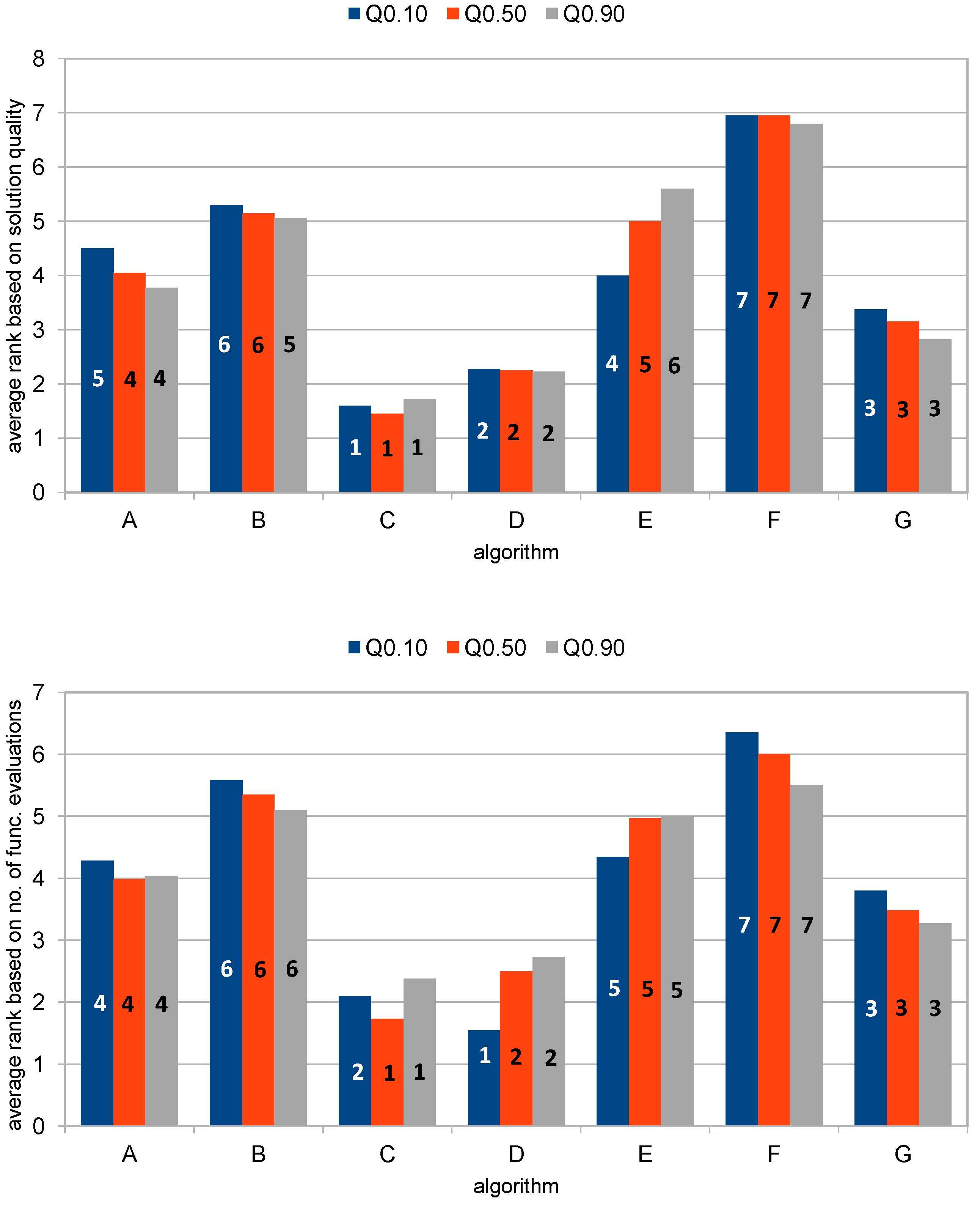
• Percentiles can be used for peak performance, average performance and bad-case performance. In the case of minimization problems for peak performance, it would be suitable to use $Q1=P_{25}$, $P_{20}$, $P_{10}$, $P_5$, etc. For average performance, it would be suitable to use the median instead of the arithmetic mean, and for bad-case performance Q3 = $P_{75}$, $P_{80}$, $P_{90}$, $P_{95}$ etc.
• Percentiles have a nice interpretation in a way that says something about the solution quality and the probability of achieving such a solution. This is in the case that computational resources such as time or the number of generated solutions is constrained, and the solution quality is the observed value; e.g., there is at least a 50% probability of achieving a solution of quality $Q_{0.5}$ or better. In a different case, when the required solution quality is specified, and time (or the number of function evaluations or some other computational resource) is the observed value, percentiles can provide data about time and probability that a specified solution will be obtained within such time; e.g., there is at least a 50% probability that a solution of the specified quality will be obtained in, at most, $Q_{0.5}$ time.
• Percentiles can take into account the common and useful practice of multiple runs of an algorithm for the same problem instance. The advantage of the stochastic nature of algorithms can be exploited in this way.

  Table 1. Probabilities for multiple runs rounded to four digits.

  No. of Runs	${\mathit{Q}}_{0.01}$	${\mathit{Q}}_{0.05}$	${\mathit{Q}}_{0.1}$	${\mathit{Q}}_{0.2}$	${\mathit{Q}}_{0.25}$	${\mathit{Q}}_{0.5}$	${\mathit{Q}}_{0.75}$	${\mathit{Q}}_{0.8}$	${\mathit{Q}}_{0.9}$	${\mathit{Q}}_{0.95}$	${\mathit{Q}}_{0.99}$
  1	0.0100	0.0500	0.1000	0.2000	0.2500	0.5000	0.7500	0.8000	0.9000	0.9500	0.9900
  2	0.0199	0.0975	0.1900	0.3600	0.4375	0.7500	0.9375	0.9600	0.9900	0.9975	0.9999
  3	0.0297	0.1426	0.2710	0.4880	0.5781	0.8750	0.9844	0.9920	0.9990	0.9999	1.0000
  4	0.0394	0.1855	0.3439	0.5904	0.6836	0.9375	0.9961	0.9984	0.9999	1.0000	1.0000
  5	0.0490	0.2262	0.4095	0.6723	0.7627	0.9688	0.9990	0.9997	1.0000	1.0000	1.0000
  10	0.0956	0.4013	0.6513	0.8926	0.9437	0.9990	1.0000	1.0000	1.0000	1.0000	1.0000
  20	0.1821	0.6415	0.8784	0.9885	0.9968	1.0000	1.0000	1.0000	1.0000	1.0000	1.0000
  30	0.2603	0.7854	0.9576	0.9988	0.9998	1.0000	1.0000	1.0000	1.0000	1.0000	1.0000
  40	0.3310	0.8715	0.9852	0.9999	1.0000	1.0000	1.0000	1.0000	1.0000	1.0000	1.0000
  50	0.3950	0.9231	0.9948	1.0000	1.0000	1.0000	1.0000	1.0000	1.0000	1.0000	1.0000
  100	0.6340	0.9941	1.0000	1.0000	1.0000	1.0000	1.0000	1.0000	1.0000	1.0000	1.0000
  200	0.8660	1.0000	1.0000	1.0000	1.0000	1.0000	1.0000	1.0000	1.0000	1.0000	1.0000
  300	0.9510	1.0000	1.0000	1.0000	1.0000	1.0000	1.0000	1.0000	1.0000	1.0000	1.0000
  400	0.9820	1.0000	1.0000	1.0000	1.0000	1.0000	1.0000	1.0000	1.0000	1.0000	1.0000
  500	0.9934	1.0000	1.0000	1.0000	1.0000	1.0000	1.0000	1.0000	1.0000	1.0000	1.0000

  contains the probabilities for a certain number of repetitions (n) and quantiles ($Q_p$), so when the algorithm is run only once, there is at least a 0.75 probability of obtaining a solution of quality $Q_{0.75}$ or better than that. When the same algorithm is repeated 10 times, there is at least a 0.9437 probability of obtaining a solution of quality $Q_{0.25}$ or better, and at least a 0.99999905 probability of achieving a solution of quality $Q_{0.75}$ or better. The probability of 0.99999905 is calculated based on the equation in [18], and is rounded to 1.0000 in Table 1.
• Percentiles can be used even when the arithmetic mean is impossible to calculate. This applies only to the case when the required solution quality is specified and the needed time (number of generated solutions, number of iterations or some other computational resources) is the observed value.
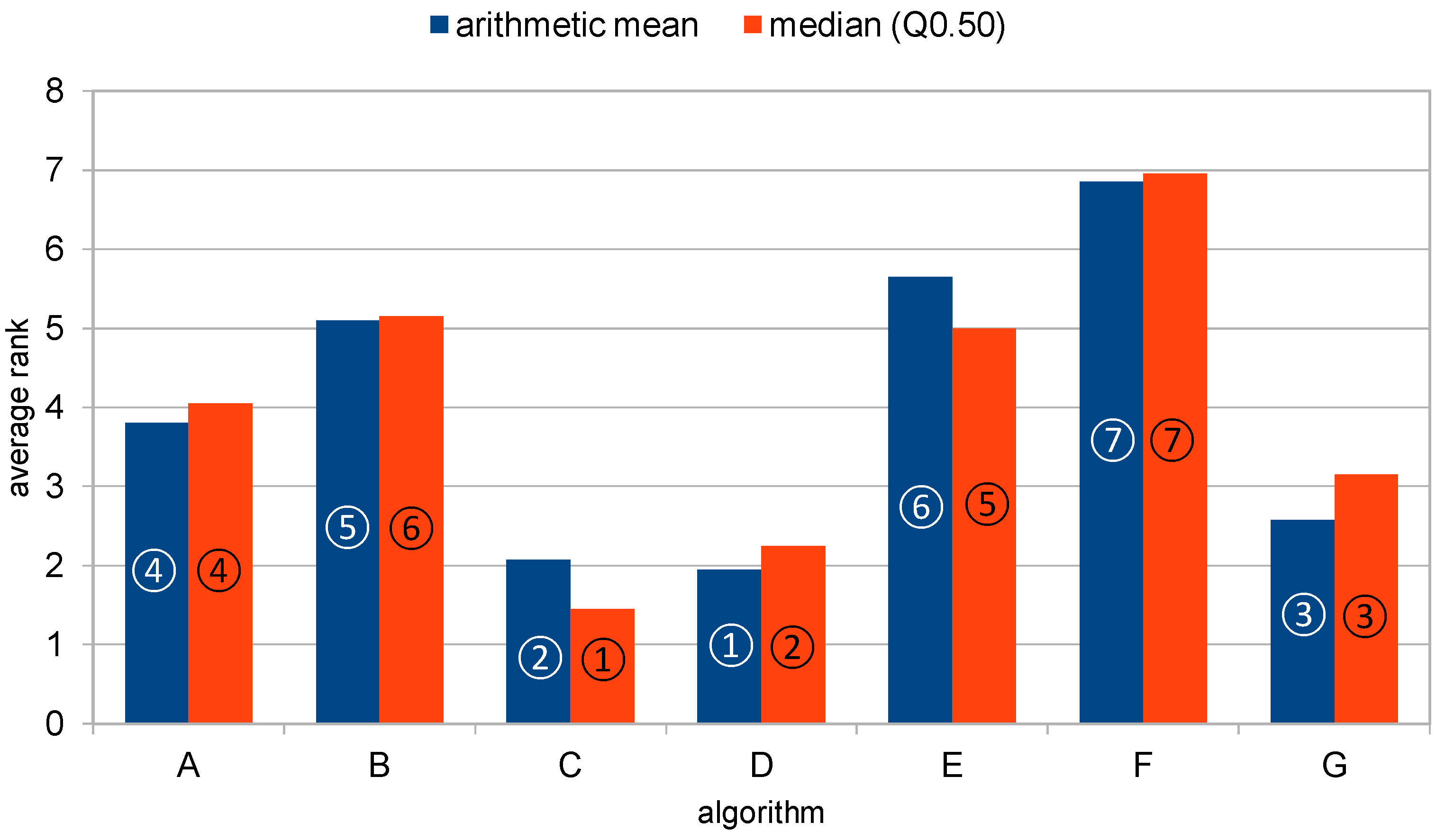
• Evolutionary computation and swarm intelligence algorithms can have very asymmetrical distribution, and a 50th percentile (median) can be more adequate than the arithmetic mean for average performance.

Median, quartiles, percentiles and other quantiles are easy to calculate manually and there are readily available functions, MEDIAN(), QUARTILE() and PERCENTILE(), in spreadsheet software such as Microsoft Excel and LibreOffice Calc. It is interesting to note that, in Microsoft Excel and Libre Office Calc, the function PERCENTILE() takes a probability that can represent a non-integer percent, and thus, actually calculate any quantile, not only percentiles.

3. Statistical Errors

If one could repeat an experiment an infinite number of times, she or he could know the true distribution and calculate the true arithmetic mean, true median and other true quantiles. In practice, it is only possible to repeat an experiment a limited number of times, get some random sample and calculate the sample mean or chosen quantiles from that sample. The calculated mean and quantiles generally differ from their true values, and usually with a larger sample, one can expect to increase accuracy, i.e., to get calculated values that are closer to the true parameters.

To make the discussion about statistical errors more explicit, let there be an algorithm and a problem instance for which true values and the experimentally obtained sample values are as follows:

• $true{Q}_{0.46}=101$
• $true{Q}_{0.50}=103$
• $trueMean=107$
• $sample{Q}_{0.50}=101$
• $sampleMean=105$.

In this case, the error for the arithmetic mean is $trueMean-sampleMean=107-105=2$. For the quantile, it is possible to consider two approaches. One way to think about the empirical estimate of the quantile is to say that the probability of $0.50$ is set as absolute, and that the error of the estimated value is $true{Q}_{0.50}-sample{Q}_{0.5}=103-101=2$. The other way is to think that value $Q_p=101$ is accurate, and that the error is made in the statement about probability p, which might be somewhat different from $0.50$. Therefore, the error made in the probability is $0.50-0.46=0.04$.

By using bootstrapping it is possible to calculate confidence intervals based on the empirical distribution of data, and not relying on some presumed theoretical distribution, e.g., normal distribution. From the experimentally obtained sample it is easy to calculate the arithmetic mean, if one exists, or a desired quantile of the sample. After that, the accuracy of this procedure can be estimated with a bootstrapping technique which can provide a standard error, a bias, and a confidence interval. The confidence interval for some statistic value ($stv$) can be calculated with the help of $stderr$ and $bias$, both obtained with the resampling of the bootstrap process. For example, normal approximation of the 68% confidence interval is defined by expression (2) and a 95% confidence interval by expression (3).

$$[stv-bias-stderr,stv-bias+stderr]$$

(2)

$$[stv-bias-1.96·stderr,stv-bias+1.96·stderr]$$

(3)

Of course, only in the case that the bias is equal to zero, expressions (2) and (3) are simplified to (4) and (5) and expression (4) is often written in a shorter way, as (6).

$$[stv-stderr,stv+stderr]$$

(4)

$$[stv-1.96·stderr,stv+1.96·stderr]$$

(5)

$$stv\pm stderr$$

(6)

However, in publications in the area of evolutionary computation and metaheuristics, currently, it is common to see a reported arithmetic mean and standard error without noting or mentioning the bias, although without any statistical tests that would confirm the apparent assumption that the bias is indeed equal to, or close to zero.

4. Experimental Research

To demonstrate our proposals in practical research, two sets of experiments were carried on the CEC2010 [32] benchmark, which contains unconstrained continuous optimization problems. It has 20 single-objective, unconstrained problem instances, named F01, F02, …, F20. For each problem instance, the number of used variables is ten ($D=10$). The nature-inspired optimization algorithms, labeled as A, B, C, D, E, F, and G, are actual implementations of the artificial bee colony (ABC) algorithm [33], the coral reefs optimization (CRO) algorithm [34], adaptive differential evolution with an optional external archive (JADE) [35], self-adaptive differential evolution (JDE) [36], particle swarm optimization (PSO) [37], the random walk algorithm (RWSi) and a self-adaptive differential evolution algorithm with population size reduction and three strategies (jDElscop) [38], respectively. For these algorithms, we used implementations from the open-source EARS project [39], including RWSi, which is a simple random walk algorithm without a learning mechanism. The algorithm F (RWSi) was used only as a baseline algorithm that we expected would, normally, always be the worst algorithm. We made the source code of all the algorithms that are used in this research publicly available at https://github.com/UM-LPM/EARS/tree/master/src/org/um/feri/ears/algorithms/so to disclose all the implementation details and to promote replication of the results by other researchers. These algorithms are just examples that we used to demonstrate the proposed methods, and to capture some of the phenomena that occur during this kind of research. We chose rather different types of algorithms with completely different origins, and also a few rather similar algorithms (three variants of differential evolution), because both situations occur in experimental research. There are, of course, a very large number of other algorithms that could have been used, such as social engineering optimizer (SEO) [40], ant inspired algorithm [41], grasshopper optimization algorithm [42], red deer algorithm (RDA) [43], quantum fruit fly optimization algorithm [44] and beetle antennae search (NABAS) algorithm [45] to name only a small fraction of the possibilities. Our experiment relied heavily on a random number generator; therefore, we used the well-tested Mersenne Twister Random Number Generator [46]. We also used the recommended parameter settings for each implemented algorithm. We did not include them in this section because we want to avoid moving the focus from the experimental methodology to the algorithms, but we have added them in the Appendix A in order to enable the replication of the conducted experiments. The reason for using labels A to G for the algorithms was to emphasize that this is not a research study about finding the best algorithm in its best implementation and parameter settings for the used problem instances. This is a research study about experimental methodology, and the algorithms are merely realistic examples. Each experiment was repeated 101 times, and, after that, the $Q_{0.50}$ (median) and arithmetic mean were calculated to assess the average performance of the algorithm. The sample size of 101 was chosen to allow simple and unambiguous calculation of different quantiles, as explained in [18]. For the peak performance we used $Q_{0.10}$, and for the bad-case performance, $Q_{0.90}$.

Two sets of experiments were performed—one with a restricted number of function evaluations in which the solution quality was the observed value—and the other in which a particular solution quality was required and the number of function evaluations was observed.

Quantiles alone can be used to evaluate or specify the performance of a stochastic algorithm on a particular problem instance, but, in addition, some statistical tests can be performed when the performance of multiple algorithms on many problem instances is of interest. For that purpose, the Friedman test can be used, along with post hoc procedures for pairwise comparison. In these procedures, quantile values can be used as input data. The Friedman test is a rank-based non-parametric statistical test that requires random data that can be ordered for each row (problem instance). This test does not require that data obey some specific distribution (such as normal distribution). Calculated percentiles, or other quantiles from a random sample, are random variables, and their values can be ordered; therefore, they can be used as the input for a Friedman test.

Since quantiles provide some guarantees about the probability of getting a certain solution quality or succeeding after a certain number of function evaluations, it might be interesting to provide some confidence intervals to quantify possible statistical errors in the assessment of true quantiles. For this purpose, we have used the bootstrapping method with 10,000 replications, and the first-order normal approximation for a 95% equi-tailed two-sided confidence interval.

The rest of this section is organized as follows. In Section 4.1, the average performance is analyzed by using the median and arithmetic mean of the solution quality. The assessment of average performance had somewhat similar results for arithmetic mean and median, but there were some discrepancies. The most important, based on the arithmetic mean, algorithm D was the best average performing, but, based on median, algorithm C was the best-performing algorithm. Further investigation of the differences between the performance of algorithm C and algorithm D is presented in Section 4.2, and their results revealed that the median was the better measure of average performance than arithmetic mean. In Section 4.3, we report the results of the average performance assessment based on observations about the required computational resources (number of function evaluations). In this case, the arithmetic mean was totally inadequate, and median proved to be a usable approach. Section 4.4 contains the results of the peak performance and bad-case performance assessments for the observed solution quality and observed number of function evaluations. In Section 4.5, we present the 95% confidence intervals for arithmetic mean, median, $Q_{0.10}$ and $Q_{0.90}$ calculated with the bootstrap method.

4.1. Average Observed Solution Quality

In this Section, we present the experiments and results acquired by limiting the number of function evaluations to 10,000 for each algorithm and observing the quality of the obtained solutions. The arithmetic means of solutions and the median solutions ($Q_{0.50}$) for the conducted experiments are presented in

Table 2. Arithmetic mean of solution quality with corresponding rank.

	Algorithm A	Algorithm B	Algorithm C	Algorithm D	Algorithm E	Algorithm F	Algorithm G
F01	$4.017\times {10}^{-7}$ (3)	$7.346\times {10}^3$ (5)	$\mathbf{1}.\mathbf{856}\times {\mathbf{10}}^{-\mathbf{10}}$(1)	$2.826\times {10}^{-9}$ (2)	$1.723\times {10}^6$ (6)	$2.346\times {10}^7$ (7)	$1.904\times {10}^{-6}$ (4)
F02	$3.034\times {10}^{-4}$ (4)	$7.954\times {10}^{-4}$ (5)	$\mathbf{0}.\mathbf{000}\times {\mathbf{10}}^{\mathbf{0}}$(1)	$1.301\times {10}^{-15}$ (2)	$1.030\times {10}^0$ (6)	$7.420\times {10}^0$ (7)	$5.972\times {10}^{-13}$ (3)
F03	$1.709\times {10}^{-5}$ (4)	$4.517\times {10}^{-1}$ (5)	$\mathbf{6}.\mathbf{236}\times {\mathbf{10}}^{-\mathbf{8}}$(1)	$4.850\times {10}^{-7}$ (2)	$3.746\times {10}^0$ (6)	$1.675\times {10}^1$ (7)	$1.221\times {10}^{-5}$ (3)
F04	$9.625\times {10}^{11}$ (7)	$5.285\times {10}^{11}$ (5)	$3.481\times {10}^9$ (3)	$1.452\times {10}^8$ (2)	$4.742\times {10}^{10}$ (4)	$9.074\times {10}^{11}$ (6)	$\mathbf{4}.\mathbf{129}\times {\mathbf{10}}^{\mathbf{6}}$(1)
F05	$1.390\times {10}^{-7}$ (4)	$2.042\times {10}^1$ (5)	$\mathbf{3}.\mathbf{399}\times {\mathbf{10}}^{-\mathbf{13}}$(1)	$1.014\times {10}^{-12}$ (2)	$3.316\times {10}^4$ (6)	$5.731\times {10}^5$ (7)	$3.241\times {10}^{-9}$ (3)
F06	$3.804\times {10}^5$ (4)	$1.149\times {10}^6$ (5)	$5.847\times {10}^0$ (3)	$\mathbf{9}.\mathbf{835}\times {\mathbf{10}}^{-\mathbf{1}}$(1)	$2.924\times {10}^6$ (6)	$1.096\times {10}^7$ (7)	$1.269\times {10}^0$ (2)
F07	$7.035\times {10}^5$ (3)	$1.086\times {10}^7$ (5)	$\mathbf{1}.\mathbf{167}\times {\mathbf{10}}^{\mathbf{5}}$(1)	$2.004\times {10}^5$ (2)	$9.351\times {10}^7$ (6)	$3.354\times {10}^8$ (7)	$8.395\times {10}^5$ (4)
F08	$1.081\times {10}^5$ (4)	$1.290\times {10}^6$ (5)	$6.664\times {10}^3$ (2)	$3.320\times {10}^4$ (3)	$1.831\times {10}^6$ (6)	$1.605\times {10}^7$ (7)	$\mathbf{4}.\mathbf{179}\times {\mathbf{10}}^{\mathbf{2}}$(1)
F09	$7.034\times {10}^5$ (7)	$4.083\times {10}^5$ (6)	$3.333\times {10}^2$ (3)	$\mathbf{2}.\mathbf{078}\times {\mathbf{10}}^{\mathbf{0}}$(1)	$1.190\times {10}^5$ (4)	$2.917\times {10}^5$ (5)	$5.228\times {10}^0$ (2)
F10	$5.405\times {10}^{-3}$ (4)	$1.682\times {10}^{-2}$ (5)	$\mathbf{8}.\mathbf{759}\times {\mathbf{10}}^{-\mathbf{15}}$(1)	$3.521\times {10}^{-11}$ (2)	$3.202\times {10}^{-1}$ (6)	$2.979\times {10}^0$ (7)	$1.405\times {10}^{-10}$ (3)
F11	$2.301\times {10}^0$ (4)	$4.155\times {10}^0$ (5)	$1.678\times {10}^{-1}$ (3)	$6.108\times {10}^{-2}$ (2)	$1.651\times {10}^1$ (6)	$2.563\times {10}^1$ (7)	$\mathbf{2}.\mathbf{876}\times {\mathbf{10}}^{-\mathbf{2}}$(1)
F12	$\mathbf{7}.\mathbf{341}\times {\mathbf{10}}^{-\mathbf{1}}$(1)	$5.364\times {10}^1$ (5)	$7.524\times {10}^0$ (4)	$1.926\times {10}^0$ (2)	$2.102\times {10}^2$ (6)	$1.683\times {10}^3$ (7)	$2.134\times {10}^0$ (3)
F13	$6.277\times {10}^{-2}$ (4)	$6.871\times {10}^{-1}$ (5)	$\mathbf{4}.\mathbf{381}\times {\mathbf{10}}^{-\mathbf{3}}$(1)	$1.987\times {10}^{-2}$ (3)	$1.091\times {10}^2$ (6)	$1.595\times {10}^3$ (7)	$4.418\times {10}^{-3}$ (2)
F14	$7.729\times {10}^4$ (5)	$6.862\times {10}^4$ (4)	$\mathbf{1}.\mathbf{088}\times {\mathbf{10}}^{-\mathbf{14}}$(1)	$1.008\times {10}^{-9}$ (2)	$1.014\times {10}^5$ (6)	$2.386\times {10}^5$ (7)	$8.303\times {10}^3$ (3)
F15	$1.764\times {10}^{-3}$ (4)	$3.948\times {10}^{-3}$ (5)	$3.518\times {10}^{-17}$ (2)	$\mathbf{0}.\mathbf{000}\times {\mathbf{10}}^{\mathbf{0}}$(1)	$9.173\times {10}^{-3}$ (6)	$5.174\times {10}^{-2}$ (7)	$4.619\times {10}^{-14}$ (3)
F16	$1.579\times {10}^0$ (5)	$1.986\times {10}^0$ (6)	$5.540\times {10}^{-11}$ (2)	$\mathbf{2}.\mathbf{721}\times {\mathbf{10}}^{-\mathbf{11}}$(1)	$1.457\times {10}^{-1}$ (4)	$6.551\times {10}^0$ (7)	$4.685\times {10}^{-8}$ (3)
F17	$7.518\times {10}^{-1}$ (3)	$6.655\times {10}^0$ (5)	$1.313\times {10}^0$ (4)	$4.867\times {10}^{-1}$ (2)	$6.236\times {10}^1$ (6)	$2.131\times {10}^2$ (7)	$\mathbf{4}.\mathbf{030}\times {\mathbf{10}}^{-\mathbf{1}}$(1)
F18	$1.173\times {10}^{-1}$ (4)	$1.216\times {10}^0$ (6)	$3.665\times {10}^{-2}$ (2.5)	$\mathbf{2}.\mathbf{263}\times {\mathbf{10}}^{-\mathbf{3}}$(1)	$6.795\times {10}^{-1}$ (5)	$4.312\times {10}^0$ (7)	$3.665\times {10}^{-2}$ (2.5)
F19	$\mathbf{4}.\mathbf{486}\times {\mathbf{10}}^{\mathbf{0}}$(1)	$7.343\times {10}^1$ (5)	$2.103\times {10}^1$ (3)	$1.506\times {10}^1$ (2)	$6.463\times {10}^2$ (6)	$1.650\times {10}^3$ (7)	$3.962\times {10}^1$ (4)
F20	$\mathbf{4}.\mathbf{919}\times {\mathbf{10}}^{-\mathbf{1}}$(1)	$1.922\times {10}^1$ (5)	$1.105\times {10}^0$ (2)	$1.429\times {10}^1$ (4)	$5.360\times {10}^1$ (6)	$2.842\times {10}^2$ (7)	$7.426\times {10}^0$ (3)
F.rank	3.8	5.1	2.075	1.95	5.65	6.85	2.575

and

Table 3. Quantiles $Q_{0.50}$ of solution quality with corresponding rank.

	Algorithm A	Algorithm B	Algorithm C	Algorithm D	Algorithm E	Algorithm F	Algorithm G
F01	$8.712\times {10}^{-8}$ (3)	$3.762\times {10}^3$ (5)	$\mathbf{3}.\mathbf{843}\times {\mathbf{10}}^{-\mathbf{11}}$(1)	$1.581\times {10}^{-9}$ (2)	$2.870\times {10}^4$ (6)	$2.206\times {10}^7$ (7)	$6.988\times {10}^{-7}$ (4)
F02	$\mathbf{0}.\mathbf{000}\times {\mathbf{10}}^{\mathbf{0}}$(2)	$5.194\times {10}^{-4}$ (5)	$\mathbf{0}.\mathbf{000}\times {\mathbf{10}}^{\mathbf{0}}$(2)	$\mathbf{0}.\mathbf{000}\times {\mathbf{10}}^{\mathbf{0}}$(2)	$4.625\times {10}^{-1}$ (6)	$7.462\times {10}^0$ (7)	$2.895\times {10}^{-13}$ (4)
F03	$1.166\times {10}^{-5}$ (4)	$3.122\times {10}^{-1}$ (5)	$\mathbf{3}.\mathbf{512}\times {\mathbf{10}}^{-\mathbf{8}}$(1)	$3.138\times {10}^{-7}$ (2)	$1.646\times {10}^0$ (6)	$1.688\times {10}^1$ (7)	$1.066\times {10}^{-5}$ (3)
F04	$6.387\times {10}^{11}$ (6)	$3.170\times {10}^{11}$ (5)	$\mathbf{1}.\mathbf{247}\times {\mathbf{10}}^{-\mathbf{1}}$(1)	$2.043\times {10}^6$ (3)	$2.451\times {10}^{10}$ (4)	$7.885\times {10}^{11}$ (7)	$7.758\times {10}^5$ (2)
F05	$3.553\times {10}^{-9}$ (4)	$1.167\times {10}^1$ (5)	$\mathbf{8}.\mathbf{882}\times {\mathbf{10}}^{-\mathbf{15}}$(1)	$2.007\times {10}^{-13}$ (2)	$1.437\times {10}^1$ (6)	$5.315\times {10}^5$ (7)	$1.154\times {10}^{-9}$ (3)
F06	$4.179\times {10}^4$ (4)	$1.647\times {10}^6$ (5)	$6.974\times {10}^{-2}$ (2)	$\mathbf{7}.\mathbf{634}\times {\mathbf{10}}^{-\mathbf{3}}$(1)	$3.574\times {10}^6$ (6)	$1.121\times {10}^7$ (7)	$1.115\times {10}^{-1}$ (3)
F07	$2.646\times {10}^5$ (3)	$6.833\times {10}^6$ (5)	$1.250\times {10}^5$ (2)	$\mathbf{1}.\mathbf{594}\times {\mathbf{10}}^{\mathbf{3}}$(1)	$4.986\times {10}^7$ (6)	$3.458\times {10}^8$ (7)	$2.781\times {10}^5$ (4)
F08	$6.012\times {10}^4$ (4)	$1.287\times {10}^6$ (5)	$\mathbf{6}.\mathbf{755}\times {\mathbf{10}}^{-\mathbf{7}}$(1)	$9.001\times {10}^3$ (3)	$3.533\times {10}^6$ (6)	$1.493\times {10}^7$ (7)	$5.067\times {10}^1$ (2)
F09	$4.411\times {10}^5$ (7)	$2.043\times {10}^5$ (5)	$\mathbf{9}.\mathbf{345}\times {\mathbf{10}}^{-\mathbf{12}}$(1)	$2.672\times {10}^{-1}$ (3)	$3.642\times {10}^4$ (4)	$2.555\times {10}^5$ (6)	$1.739\times {10}^{-1}$ (2)
F10	$3.258\times {10}^{-3}$ (5)	$6.416\times {10}^{-3}$ (6)	$\mathbf{0}.\mathbf{000}\times {\mathbf{10}}^{\mathbf{0}}$(1)	$1.371\times {10}^{-11}$ (3)	$1.776\times {10}^{-15}$ (2)	$2.960\times {10}^0$ (7)	$5.782\times {10}^{-11}$ (4)
F11	$2.256\times {10}^0$ (4)	$3.382\times {10}^0$ (5)	$\mathbf{1}.\mathbf{269}\times {\mathbf{10}}^{-\mathbf{5}}$(1)	$3.146\times {10}^{-3}$ (2)	$1.997\times {10}^1$ (6)	$2.581\times {10}^1$ (7)	$6.880\times {10}^{-3}$ (3)
F12	$2.567\times {10}^{-1}$ (4)	$2.934\times {10}^1$ (5)	$\mathbf{1}.\mathbf{561}\times {\mathbf{10}}^{-\mathbf{1}}$(1.5)	$\mathbf{1}.\mathbf{561}\times {\mathbf{10}}^{-\mathbf{1}}$(1.5)	$1.643\times {10}^2$ (6)	$1.697\times {10}^3$ (7)	$1.562\times {10}^{-1}$ (3)
F13	$3.432\times {10}^{-2}$ (4)	$4.332\times {10}^{-1}$ (5)	$\mathbf{1}.\mathbf{882}\times {\mathbf{10}}^{-\mathbf{12}}$(1)	$1.673\times {10}^{-3}$ (3)	$2.386\times {10}^0$ (6)	$1.596\times {10}^3$ (7)	$1.236\times {10}^{-3}$ (2)
F14	$4.931\times {10}^4$ (6)	$1.844\times {10}^4$ (5)	$\mathbf{1}.\mathbf{057}\times {\mathbf{10}}^{-\mathbf{20}}$(1)	$7.653\times {10}^{-14}$ (2)	$1.859\times {10}^3$ (4)	$1.983\times {10}^5$ (7)	$4.640\times {10}^{-5}$ (3)
F15	$5.854\times {10}^{-4}$ (5)	$1.757\times {10}^{-3}$ (6)	$\mathbf{0}.\mathbf{000}\times {\mathbf{10}}^{\mathbf{0}}$(1.5)	$\mathbf{0}.\mathbf{000}\times {\mathbf{10}}^{\mathbf{0}}$(1.5)	$1.776\times {10}^{-15}$ (3)	$4.990\times {10}^{-2}$ (7)	$5.329\times {10}^{-15}$ (4)
F16	$1.859\times {10}^0$ (5)	$1.918\times {10}^0$ (6)	$7.944\times {10}^{-12}$ (2)	$1.119\times {10}^{-11}$ (3)	$\mathbf{1}.\mathbf{684}\times {\mathbf{10}}^{-\mathbf{12}}$(1)	$6.452\times {10}^0$ (7)	$1.650\times {10}^{-8}$ (4)
F17	$2.202\times {10}^{-1}$ (4)	$3.126\times {10}^{-1}$ (5)	$1.360\times {10}^{-5}$ (3)	$\mathbf{2}.\mathbf{910}\times {\mathbf{10}}^{-\mathbf{11}}$(1)	$2.926\times {10}^1$ (6)	$2.192\times {10}^2$ (7)	$2.950\times {10}^{-9}$ (2)
F18	$7.897\times {10}^{-2}$ (5)	$1.357\times {10}^0$ (6)	$\mathbf{5}.\mathbf{690}\times {\mathbf{10}}^{-\mathbf{22}}$(1)	$5.458\times {10}^{-11}$ (2)	$4.180\times {10}^{-3}$ (4)	$4.340\times {10}^0$ (7)	$2.865\times {10}^{-8}$ (3)
F19	$\mathbf{2}.\mathbf{376}\times {\mathbf{10}}^{\mathbf{0}}$(1)	$2.735\times {10}^1$ (4)	$8.112\times {10}^0$ (2)	$8.170\times {10}^0$ (3)	$6.584\times {10}^2$ (6)	$1.684\times {10}^3$ (7)	$3.150\times {10}^1$ (5)
F20	$\mathbf{2}.\mathbf{332}\times {\mathbf{10}}^{-\mathbf{1}}$(1)	$1.788\times {10}^1$ (5)	$2.443\times {10}^{-1}$ (2)	$1.563\times {10}^1$ (4)	$2.113\times {10}^1$ (6)	$2.755\times {10}^2$ (7)	$7.678\times {10}^0$ (3)
F.rank	4.05	5.15	1.45	2.25	5	6.95	3.15

, respectively. The number in the parentheses represents the rank that a particular algorithm achieved for the selected problem instance when compared with other algorithms on the same problem instance. The best algorithm for a particular problem instance, marked with bold font in the Tables, is normally ranked with 1, and the worst is ranked with 7, e.g., algorithm C for F07 achieved rank 1 in terms of mean solution, since it performed better than any other tested algorithm (Table 2). In some cases, multiple algorithms shared the best rank for a particular problem instance. For example, algorithm C and algorithm G shared the second and third places and had the rank 2.5 for the problem instance F18 (Table 3). At the bottom row of each Table, there is an average rank for a particular algorithm that can be used in a Friedman test.

When it comes to arithmetic mean, algorithm D was the best-ranked algorithm, followed by algorithms C, G, A, B, E, F. In the ranking based on median, the best algorithm was algorithm C, followed by algorithms D, G, A, E, B and F. These results are illustrated in Figure 1. As expected, algorithm F (RWSi), which was used as the baseline algorithm, was ranked in the last position by both approaches. The results suggest that there was a rather high agreement between arithmetic mean and median ($Q_{0.50}$) in the average performance assessment. However, there is an important disagreement in the decision as to which algorithm achieved the best average performance. For arithmetic mean, this was algorithm D, but for median, this was algorithm C. This issue is investigated further in the following Section.

4.2. Disagreement of Mean and Median

A deeper investigation of algorithmic performance was carried out due to the discrepancies between arithmetic mean and median ($Q_{0.50}$) for algorithms C and D. By comparing the data from Table 2 and Table 3, it is evident that the arithmetic mean and median disagree about the manifested performance of algorithms C and D for problem instances F04, F07, F09, F11, F18 and F19. For other problem instances, arithmetic mean and median agreed which is better—algorithm C or algorithm D. Thus, it was necessary to conduct a deeper analysis only for the affected instances.

A pairwise comparison of algorithms C and D based on complete lists of the obtained solutions sorted by solution quality for a particular problem instance is shown in Figure 2. The numbers on the abscissa represent the position of the solution in the sorted list. The best solution is the first in the list (number 1) and the worst solution is the last in the list (number 101). The ordinates show the solution quality in a logarithmic scale, due to huge differences between the best and the worst solutions.

For problem instance F04, the arithmetic mean suggests that algorithm D was better than algorithm C, and median suggests the opposite (Table 2 and Table 3). However, the results presented in Figure 2 reveal that algorithm C outperformed algorithm D significantly, which is in agreement with the median and in disagreement with the arithmetic mean. There were 82 solutions (out of 101) obtained by algorithm C that were better than the best solution obtained by algorithm D. When comparing the two sorted lists, algorithm D has a better solution than algorithm C only in place 94. Only in a few rare cases for which algorithm C obtained the worst solutions did the arithmetic mean fail in comparing algorithms C and D.

For most of the other problem instances, F07, F09, F11 and F18, a detailed analysis revealed that median made a good judgment and arithmetic mean failed. In some cases, this was even more emphasized than in the case of F04, but for F07, this is less visible from the graph in Figure 2, since the two lines are close to each other. Actually, for F07, algorithm D found 33 solutions that were better than the best solution found by algorithm C, and, moreover, only in positions 100 and 101 did algorithm C have better solutions than algorithm D.

The only problem instance for which the detailed analyses of the complete list of solutions did not provide an obvious verdict was F19. Based on the obtained lists of solutions, it is hard to decide for this instance which algorithm was better—algorithm C or algorithm D. They both showed similar performance, and perhaps the decision depends on personal preference.

Taking into consideration that, for five out of six interesting problem instances, the median provided an adequate assessment and the arithmetic mean failed, and in only one case the discrepancy between median and arithmetic mean could not be resolved, it seems that the median was more successful in evaluating algorithmic performance than the arithmetic mean.

4.3. Average Observed Number of Function Evaluations

In this Section, we report the average performance based on the second set of experiments, where a particular solution quality was specified, an optimal solution with the precision of ${10}^{-1}$, and the number of function evaluations was the observed quantity. This was possible since, for all problem instances, the optimal solutions were known. When the algorithm did not reach such solution after 100,000 function evaluations, the algorithm was interrupted as unsuccessful.

The major issue with this approach is how to deal with executions of the algorithm that cannot find solutions of required quality for an unacceptably long time. In these cases, the algorithm has to be interrupted, and these runs can be declared unsuccessful. It is obvious if the algorithm was interrupted after 100,000 function evaluations that the algorithm would need more than 100,000 function evaluations, and possibly an infinite number of evaluations to reach the desired solution quality.

Unfortunately, it is rather common to see published results where this fact is ignored completely. Some researchers simply calculate the arithmetic mean only from successful runs, or take into account the number of function evaluations after which the algorithm was interrupted as if it was a successful run. To illustrate such inadequate practice, we have presented “results” this way in

Table 4. Arithmetic mean of the required number of function evaluations with corresponding rank when unsuccessfu cases are simply ignored—the wrong way to report results.

	Algorithm A	Algorithm B	Algorithm C	Algorithm D	Algorithm E	Algorithm F	Algorithm G
F01	5417 (5)	53920 (7)	4654 (3)	3730 (2)	5173 (4)	1 (1)	7446 (6)
F02	1264 (4)	3433 (6)	9855 (2)	1027 (3)	8842 (1)	n/a (7)	1720 (5)
F03	4735 (4)	12800 (6)	2900 (3)	2402 (2)	2228 (1)	n/a (7)	4996 (5)
F04	n/a (5.5)	n/a (5.5)	11450 (1)	68470 (3)	n/a (5.5)	n/a (5.5)	29860 (2)
F05	4537 (3)	19820 (6)	3323 (2)	2604 (1)	5471 (5)	n/a (7)	4954 (4)
F06	52350 (4)	n/a (6)	10640 (2)	6566 (1)	n/a (6)	n/a (6)	13320 (3)
F07	47830 (4)	n/a (6)	13080 (2)	7262 (1)	n/a (6)	n/a (6)	18230 (3)
F08	n/a (5.5)	n/a (5.5)	8313 (1)	15130 (2)	n/a (5.5)	n/a (5.5)	19570 (3)
F09	n/a (5.5)	n/a (5.5)	6110 (1)	15630 (3)	n/a (5.5)	n/a (5.5)	12590 (2)
F10	2213 (5)	4195 (6)	9964 (2)	1025 (3)	7982 (1)	n/a (7)	1794 (4)
F11	27390 (6)	24840 (5)	5549 (3)	4821 (2)	4128 (1)	n/a (7)	9301 (4)
F12	27310 (5)	39460 (6)	7647 (2)	4337 (1)	17430 (4)	n/a (7)	10460 (3)
F13	7259 (4)	11510 (6)	4168 (2)	5003 (3)	3705 (1)	n/a (7)	7555 (5)
F14	n/a (6)	n/a (6)	3960 (1)	4124 (2)	48030 (4)	n/a (6)	8014 (3)
F15	7702 (6)	7197 (5)	2439 (3)	2152 (2)	1977 (1)	3698 (7)	3027 (4)
F16	42300 (6)	25410 (5)	2016 (3)	1298 (1)	1669 (2)	n/a (7)	3060 (4)
F17	26240 (5)	26580 (6)	6754 (3)	3599 (2)	3458 (1)	n/a (7)	11040 (4)
F18	12220 (6)	9326 (5)	2734 (1)	3701 (3)	3616 (2)	n/a (7)	4042 (4)
F19	48880 (4)	66980 (5)	15540 (2)	9494 (1)	n/a (6.5)	n/a (6.5)	27190 (3)
F20	20310 (2)	20740 (3)	10420 (1)	38800 (5)	n/a (6.5)	n/a (6.5)	31620 (4)
F.rank	4.78	5.58	2	2.15	3.48	6.28	3.75

. In this case, out of 140 results in this Table, 61 are reported incorrectly. The wrongly reported results are emphasized in the text by a bold font. If we had used the limiting number of function evaluations instead (100,000), there would be 96 wrongly reported results out of 140 results.

The most ridiculous example of such malpractice occurred for the problem instance F01 in Table 4. Here, the algorithm F (RWSi) had the best result! The arithmetic mean of the required number of function evaluations was one. This is a very puzzling result, taking into account that other algorithms needed thousands or tens of thousands of function evaluations to obtain the specified solution quality. The secret of “such success” is revealed in

Table 5. Success rate (SR).

	Algorithm A	Algorithm B	Algorithm C	Algorithm D	Algorithm E	Algorithm F	Algorithm G
F01	100%	83%	100%	100%	24%	1%	100%
F02	100%	100%	100%	100%	36%	0%	100%
F03	100%	100%	100%	97%	35%	0%	100%
F04	0%	0%	100%	70%	0%	0%	100%
F05	100%	100%	100%	100%	17%	0%	100%
F06	83%	0%	87%	91%	0%	0%	95%
F07	69%	0%	39%	20%	0%	0%	49%
F08	0%	0%	100%	99%	0%	0%	98%
F09	0%	0%	100%	99%	0%	0%	100%
F10	100%	100%	100%	100%	66%	0%	100%
F11	4%	3%	95%	79%	2%	0%	100%
F12	97%	16%	50%	22%	1%	0%	33%
F13	99%	41%	100%	100%	18%	0%	100%
F14	0%	0%	100%	98%	2%	0%	99%
F15	100%	100%	100%	100%	100%	100%	100%
F16	57%	57%	100%	100%	95%	0%	100%
F17	97%	65%	67%	31%	2%	0%	68%
F18	98%	15%	98%	99%	89%	0%	99%
F19	78%	2%	58%	27%	0%	0%	71%
F20	100%	15%	85%	54%	0%	0%	52%

, where we reported the success rate. Out of 101 runs, algorithm F (RWSi) succeeded only once, and that was in the first iteration of the algorithm, so the arithmetic mean of successful runs seems incredibly good. Obviously, knowing the whole story, it is very unlikely that some researchers would consider the algorithm F (RWSi) to be the best algorithm for F01. This ridiculous situation also happened for some other problem instances, e.g., for F11 algorithm E, the mean number of the function evaluations for successful runs was 4128, which was better (ranked) than D, which had 4821, although the success rate for algorithm E was only 2%, and for algorithm D, it was 79% (Table 5).

The correct way to report arithmetic mean is shown in

Table 6. Arithmetic mean of the required number of solutions—the correct way.

	Algorithm A	Algorithm B	Algorithm C	Algorithm D	Algorithm E	Algorithm F	Algorithm G
F01	5417	n/a	4654	3730	n/a	n/a	7446
F02	1264	3433	985.5	1027	n/a	n/a	1720
F03	4735	12800	2900	n/a	n/a	n/a	4996
F04	n/a	n/a	11450	n/a	n/a	n/a	29860
F05	4537	19820	3323	2604	n/a	n/a	4954
F06	n/a	n/a	n/a	n/a	n/a	n/a	n/a
F07	n/a	n/a	n/a	n/a	n/a	n/a	n/a
F08	n/a	n/a	8313	n/a	n/a	n/a	n/a
F09	n/a	n/a	6110	n/a	n/a	n/a	12590
F10	2213	4195	996.4	1025	n/a	n/a	1794
F11	n/a	n/a	n/a	n/a	n/a	n/a	9301
F12	n/a	n/a	n/a	n/a	n/a	n/a	n/a
F13	n/a	n/a	4168	5003	n/a	n/a	7555
F14	n/a	n/a	3960	n/a	n/a	n/a	n/a
F15	770.2	719.7	243.9	215.2	197.7	3698	302.7
F16	n/a	n/a	2016	1298	n/a	n/a	3060
F17	n/a	n/a	n/a	n/a	n/a	n/a	n/a
F18	n/a	n/a	n/a	n/a	n/a	n/a	n/a
F19	n/a	n/a	n/a	n/a	n/a	n/a	n/a
F20	20310	n/a	n/a	n/a	n/a	n/a	n/a
F.rank	n/a	n/a	n/a	n/a	n/a	n/a	n/a

. However, ranking n/a results should be conducted with special caution. In general, these results are unknown, but not necessarily worse than other results for a particular problem instance. So, here, another serious problem arises. The whole ranking for this problem instance may be compromised because of maybe only one n/a result in the row (for one problem instance). Unfortunately, because of the many n/a results in Table 6, it is impractical or impossible to assess algorithmic performance correctly based on the arithmetic mean.

The medians ($Q_{0.50}$) of the required number of function evaluations needed to obtain the specified solution quality are presented in

Table 7. Median ($Q_{0.50}$) of the required number of solution evaluations with corresponding rank.

	Algorithm A	Algorithm B	Algorithm C	Algorithm D	Algorithm E	Algorithm F	Algorithm G
F01	5415 (3)	57490 (5)	4618 (2)	3670 (1)	$>{10}^5$ (6.5)	$>{10}^5$ (6.5)	7455 (4)
F02	1238 (3)	3320 (5)	979 (1)	1002 (2)	$>{10}^5$ (6.5)	$>{10}^5$ (6.5)	1727 (4)
F03	4729 (3)	12840 (5)	2897 (2)	2418 (1)	$>{10}^5$ (6.5)	$>{10}^5$ (6.5)	4967 (4)
F04	$>{10}^5$ (5.5)	$>{10}^5$ (5.5)	10800 (1)	79390 (3)	$>{10}^5$ (5.5)	$>{10}^5$ (5.5)	29770 (2)
F05	4535 (3)	19820 (5)	3302 (2)	2539 (1)	$>{10}^5$ (6.5)	$>{10}^5$ (6.5)	4940 (4)
F06	56480 (4)	$>{10}^5$ (6)	9671 (2)	6069 (1)	$>{10}^5$ (6)	$>{10}^5$ (6)	12190 (3)
F07	66490 (1)	$>{10}^5$ (4.5)	$>{10}^5$ (4.5)	$>{10}^5$ (4.5)	$>{10}^5$ (4.5)	$>{10}^5$ (4.5)	$>{10}^5$ (4.5)
F08	$>{10}^5$ (5.5)	$>{10}^5$ (5.5)	7876 (1)	15240 (2)	$>{10}^5$ (5.5)	$>{10}^5$ (5.5)	19360 (3)
F09	$>{10}^5$ (5.5)	$>{10}^5$ (5.5)	5494 (1)	13610 (3)	$>{10}^5$ (5.5)	$>{10}^5$ (5.5)	12530 (2)
F10	2044 (5)	4039 (6)	1001 (2)	1026 (3)	893 (1)	$>{10}^5$ (7)	1790 (4)
F11	$>{10}^5$ (5.5)	$>{10}^5$ (5.5)	5200 (2)	4846 (1)	$>{10}^5$ (5.5)	$>{10}^5$ (5.5)	9391 (3)
F12	23940 (2)	$>{10}^5$ (5)	9729 (1)	$>{10}^5$ (5)	$>{10}^5$ (5)	$>{10}^5$ (5)	$>{10}^5$ (5)
F13	5320 (3)	$>{10}^5$ (6)	4085 (1)	4141 (2)	$>{10}^5$ (6)	$>{10}^5$ (6)	7518 (4)
F14	$>{10}^5$ (5.5)	$>{10}^5$ (5.5)	3988 (2)	3400 (1)	$>{10}^5$ (5.5)	$>{10}^5$ (5.5)	7987 (3)
F15	655 (6)	648 (5)	250 (3)	216 (2)	193 (1)	2903 (7)	297 (4)
F16	80250 (6)	45030 (5)	1991 (3)	1286 (1)	1502 (2)	$>{10}^5$ (7)	3028 (4)
F17	22450 (3)	42240 (4)	7542 (1)	$>{10}^5$ (6)	$>{10}^5$ (6)	$>{10}^5$ (6)	8302 (2)
F18	7069 (5)	$>{10}^5$ (6.5)	2617 (1)	3237 (2)	3818 (3)	$>{10}^5$ (6.5)	3993 (4)
F19	60170 (3)	$>{10}^5$ (5.5)	17710 (1)	$>{10}^5$ (5.5)	$>{10}^5$ (5.5)	$>{10}^5$ (5.5)	28450 (2)
F20	14950 (2)	$>{10}^5$ (6)	10730 (1)	61880 (3)	$>{10}^5$ (6)	$>{10}^5$ (6)	93080 (4)
F.rank	3.98	5.35	1.73	2.5	4.97	6	3.48

. When using quantiles, there are no n/a results, but there are some $>{10}^5$ results. In these cases, it is known that their value is larger than the prespecified value, but the exact value cannot be calculated. It is important to observe that the number of n/a in Table 6 is 96, and the number of $>{10}^5$ results for median is 59. More usable results in the case of median when compared with arithmetic mean were expected, and can be explained easily by taking the success rate into consideration (Table 5).

It is useful to note that $>{10}^5$ for quantiles is a more usable result than n/a for arithmetic mean. In addition, it is important to note that $>{10}^5$ cannot compromise the whole row (the results for one problem instance) as n/a in the case of arithmetic mean can. However there is one subtle question. What about different $>{10}^5$ results for some particular problem instance? Is it suitable to give them equal ranking, since we do not know the exact values of the quantiles? One way of proceeding with this is that the researcher or practitioner decides that all $>{10}^5$ are unacceptable and equally bad; thus, equal ranking is suitable. Alternatively, perhaps some additional criteria could be used to rank these $>{10}^5$ solutions between themselves, such as the success rate or the quality of the obtained solutions. In our report, we have chosen the first possibility.

4.4. Peak Performance and Bad-Case Performance

In order to assess the peak performance of the algorithms we calculated $Q_{0.10}$, and for bad-case performance, we calculated $Q_{0.90}$. The assessment was conducted on two sets of performed experiments. In the first set of experiments, the number of function evaluations was set to 10,000 and the quality of solution was the observed value. In the second set of experiments, the optimal solution within ${10}^{-1}$ precision was required, and the number of function evaluations was the observed value.

The results of the experiments with $Q_{0.10}$ and $Q_{0.90}$ of the observed solution quality are presented in

Table 8. Quantiles $Q_{0.10}$ of the obtained solution quality.

	Algorithm A	Algorithm B	Algorithm C	Algorithm D	Algorithm E	Algorithm F	Algorithm G
F01	$5.736\times {10}^{-9}$ (4)	$6.637\times {10}^2$ (6)	$3.274\times {10}^{-12}$ (2)	$3.187\times {10}^{-10}$ (3)	$\mathbf{6}.\mathbf{283}\times {\mathbf{10}}^{-\mathbf{14}}$(1)	$8.679\times {10}^6$ (7)	$1.109\times {10}^{-7}$ (5)
F02	$\mathbf{0}.\mathbf{000}\times {\mathbf{10}}^{\mathbf{0}}$(2)	$2.516\times {10}^{-4}$ (5)	$\mathbf{0}.\mathbf{000}\times {\mathbf{10}}^{\mathbf{0}}$ (2)	$\mathbf{0}.\mathbf{000}\times {\mathbf{10}}^{\mathbf{0}}$(2)	$3.065\times {10}^{-2}$ (6)	$5.009\times {10}^0$ (7)	$4.974\times {10}^{-14}$ (4)
F03	$4.453\times {10}^{-6}$ (5)	$1.485\times {10}^{-1}$ (6)	$1.282\times {10}^{-8}$ (2)	$1.456\times {10}^{-7}$ (3)	$\mathbf{1}.\mathbf{175}\times {\mathbf{10}}^{-\mathbf{10}}$(1)	$1.562\times {10}^1$ (7)	$3.920\times {10}^{-6}$ (4)
F04	$1.581\times {10}^{11}$ (6)	$9.777\times {10}^{10}$ (5)	$\mathbf{2}.\mathbf{340}\times {\mathbf{10}}^{-\mathbf{4}}$(1)	$8.599\times {10}^4$ (2)	$4.994\times {10}^9$ (4)	$2.772\times {10}^{11}$ (7)	$1.237\times {10}^5$ (3)
F05	$8.882\times {10}^{-15}$ (3)	$3.252\times {10}^0$ (6)	$\mathbf{0}.\mathbf{000}\times {\mathbf{10}}^{\mathbf{0}}$(1)	$7.105\times {10}^{-15}$ (2)	$1.421\times {10}^{-14}$ (4)	$2.834\times {10}^5$ (7)	$9.947\times {10}^{-11}$ (5)
F06	$4.009\times {10}^3$ (5)	$2.053\times {10}^4$ (6)	$4.272\times {10}^{-3}$ (2)	$\mathbf{2}.\mathbf{406}\times {\mathbf{10}}^{-\mathbf{3}}$(1)	$2.196\times {10}^1$ (4)	$8.708\times {10}^6$ (7)	$3.775\times {10}^{-2}$ (3)
F07	$1.251\times {10}^5$ (4)	$1.371\times {10}^5$ (5)	$1.144\times {10}^2$ (2)	$\mathbf{1}.\mathbf{412}\times {\mathbf{10}}^{\mathbf{0}}$(1)	$7.007\times {10}^6$ (6)	$2.138\times {10}^8$ (7)	$1.249\times {10}^5$ (3)
F08	$1.048\times {10}^4$ (4)	$3.044\times {10}^4$ (6)	$\mathbf{4}.\mathbf{666}\times {\mathbf{10}}^{-\mathbf{10}}$(1)	$6.986\times {10}^1$ (3)	$1.777\times {10}^4$ (5)	$7.102\times {10}^6$ (7)	$4.217\times {10}^0$ (2)
F09	$1.010\times {10}^5$ (7)	$2.198\times {10}^4$ (5)	$\mathbf{2}.\mathbf{596}\times {\mathbf{10}}^{-\mathbf{14}}$(1)	$1.503\times {10}^{-2}$ (2)	$2.135\times {10}^3$ (4)	$8.667\times {10}^4$ (6)	$1.579\times {10}^{-2}$ (3)
F10	$4.499\times {10}^{-4}$ (5)	$6.742\times {10}^{-4}$ (6)	$\mathbf{0}.\mathbf{000}\times {\mathbf{10}}^{\mathbf{0}}$(1.5)	$1.203\times {10}^{-12}$ (3)	$\mathbf{0}.\mathbf{000}\times {\mathbf{10}}^{\mathbf{0}}$(1.5)	$1.875\times {10}^0$ (7)	$1.091\times {10}^{-11}$ (4)
F11	$1.145\times {10}^0$ (5)	$9.015\times {10}^{-1}$ (4)	$\mathbf{1}.\mathbf{655}\times {\mathbf{10}}^{-\mathbf{7}}$(1)	$8.495\times {10}^{-4}$ (2)	$2.606\times {10}^0$ (6)	$2.385\times {10}^1$ (7)	$2.724\times {10}^{-3}$ (3)
F12	$5.486\times {10}^{-2}$ (4)	$1.034\times {10}^0$ (5)	$3.266\times {10}^{-5}$ (2)	$\mathbf{1}.\mathbf{010}\times {\mathbf{10}}^{-\mathbf{7}}$(1)	$1.692\times {10}^1$ (6)	$1.258\times {10}^3$ (7)	$1.162\times {10}^{-4}$ (3)
F13	$8.052\times {10}^{-3}$ (5)	$1.317\times {10}^{-1}$ (6)	$\mathbf{4}.\mathbf{960}\times {\mathbf{10}}^{-\mathbf{15}}$(1)	$1.205\times {10}^{-5}$ (2)	$7.620\times {10}^{-3}$ (4)	$9.066\times {10}^2$ (7)	$3.710\times {10}^{-5}$ (3)
F14	$6.843\times {10}^3$ (6)	$1.959\times {10}^3$ (5)	$\mathbf{3}.\mathbf{760}\times {\mathbf{10}}^{-\mathbf{24}}$(1)	$1.017\times {10}^{-16}$ (2)	$1.948\times {10}^2$ (4)	$6.106\times {10}^4$ (7)	$2.746\times {10}^{-6}$ (3)
F15	$7.448\times {10}^{-5}$ (6)	$5.104\times {10}^{-5}$ (5)	$\mathbf{0}.\mathbf{000}\times {\mathbf{10}}^{\mathbf{0}}$(2.5)	$\mathbf{0}.\mathbf{000}\times {\mathbf{10}}^{\mathbf{0}}$(2.5)	$\mathbf{0}.\mathbf{000}\times {\mathbf{10}}^{\mathbf{0}}$(2.5)	$1.794\times {10}^{-2}$ (7)	$\mathbf{0}.\mathbf{000}\times {\mathbf{10}}^{\mathbf{0}}$(2.5)
F16	$3.478\times {10}^{-1}$ (6)	$8.915\times {10}^{-2}$ (5)	$8.953\times {10}^{-13}$ (2)	$1.915\times {10}^{-12}$ (3)	$\mathbf{3}.\mathbf{304}\times {\mathbf{10}}^{-\mathbf{13}}$(1)	$5.064\times {10}^0$ (7)	$3.541\times {10}^{-9}$ (4)
F17	$1.309\times {10}^{-1}$ (5)	$1.681\times {10}^{-2}$ (4)	$6.173\times {10}^{-10}$ (3)	$\mathbf{0}.\mathbf{000}\times {\mathbf{10}}^{\mathbf{0}}$(1)	$3.122\times {10}^{-1}$ (6)	$1.255\times {10}^2$ (7)	$4.547\times {10}^{-13}$ (2)
F18	$1.196\times {10}^{-2}$ (5)	$5.745\times {10}^{-2}$ (6)	$\mathbf{3}.\mathbf{545}\times {\mathbf{10}}^{-\mathbf{26}}$(1)	$8.721\times {10}^{-16}$ (2)	$1.880\times {10}^{-3}$ (4)	$2.274\times {10}^0$ (7)	$4.060\times {10}^{-10}$ (3)
F19	$\mathbf{2}.\mathbf{035}\times {\mathbf{10}}^{-\mathbf{1}}$(1)	$3.826\times {10}^0$ (4)	$6.749\times {10}^{-1}$ (2)	$2.009\times {10}^0$ (3)	$3.429\times {10}^2$ (6)	$1.452\times {10}^3$ (7)	$1.276\times {10}^1$ (5)
F20	$9.206\times {10}^{-2}$ (2)	$5.977\times {10}^0$ (6)	$\mathbf{1}.\mathbf{666}\times {\mathbf{10}}^{-\mathbf{3}}$(1)	$4.214\times {10}^0$ (5)	$3.188\times {10}^{-1}$ (4)	$1.821\times {10}^2$ (7)	$2.708\times {10}^{-1}$ (3)
F.rank	4.5	5.3	1.6	2.275	4	6.95	3.375

and

Table 9. Quantiles $Q_{0.90}$ of the obtained solution quality.

	Algorithm A	Algorithm B	Algorithm C	Algorithm D	Algorithm E	Algorithm F	Algorithm G
F01	$4.907\times {10}^{-7}$ (3)	$2.089\times {10}^4$ (5)	$\mathbf{3}.\mathbf{404}\times {\mathbf{10}}^{-\mathbf{10}}$(1)	$5.955\times {10}^{-9}$ (2)	$4.073\times {10}^6$ (6)	$3.632\times {10}^7$ (7)	$4.135\times {10}^{-6}$ (4)
F02	$3.553\times {10}^{-15}$ (2.5)	$1.425\times {10}^{-3}$ (5)	$\mathbf{0}.\mathbf{000}\times {\mathbf{10}}^{\mathbf{0}}$(1)	$3.553\times {10}^{-15}$ (2.5)	$2.752\times {10}^0$ (6)	$9.772\times {10}^0$ (7)	$1.322\times {10}^{-12}$ (4)
F03	$3.775\times {10}^{-5}$ (4)	$1.204\times {10}^0$ (5)	$\mathbf{1}.\mathbf{622}\times {\mathbf{10}}^{-\mathbf{7}}$(1)	$9.327\times {10}^{-7}$ (2)	$8.279\times {10}^0$ (6)	$1.785\times {10}^1$ (7)	$2.209\times {10}^{-5}$ (3)
F04	$2.282\times {10}^{12}$ (7)	$1.233\times {10}^{12}$ (5)	$\mathbf{5}.\mathbf{290}\times {\mathbf{10}}^{\mathbf{6}}$(1)	$7.970\times {10}^7$ (3)	$1.059\times {10}^{11}$ (4)	$1.621\times {10}^{12}$ (6)	$1.075\times {10}^7$ (2)
F05	$1.190\times {10}^{-7}$ (4)	$3.977\times {10}^1$ (5)	$\mathbf{5}.\mathbf{524}\times {\mathbf{10}}^{-\mathbf{13}}$(1)	$2.292\times {10}^{-12}$ (2)	$4.296\times {10}^1$ (6)	$9.127\times {10}^5$ (7)	$6.659\times {10}^{-9}$ (3)
F06	$1.675\times {10}^6$ (4)	$2.319\times {10}^6$ (5)	$2.001\times {10}^1$ (3)	$\mathbf{4}.\mathbf{300}\times {\mathbf{10}}^{-\mathbf{2}}$(1)	$3.897\times {10}^6$ (6)	$1.294\times {10}^7$ (7)	$1.624\times {10}^0$ (2)
F07	$8.888\times {10}^5$ (3)	$3.014\times {10}^7$ (5)	$2.499\times {10}^5$ (2)	$\mathbf{2}.\mathbf{498}\times {\mathbf{10}}^{\mathbf{5}}$(1)	$2.504\times {10}^8$ (6)	$4.542\times {10}^8$ (7)	$1.774\times {10}^6$ (4)
F08	$2.496\times {10}^5$ (4)	$2.696\times {10}^6$ (5)	$\mathbf{2}.\mathbf{633}\times {\mathbf{10}}^{-\mathbf{1}}$(1)	$9.851\times {10}^4$ (3)	$3.577\times {10}^6$ (6)	$2.645\times {10}^7$ (7)	$7.539\times {10}^2$ (2)
F09	$1.520\times {10}^6$ (7)	$1.024\times {10}^6$ (6)	$\mathbf{2}.\mathbf{198}\times {\mathbf{10}}^{-\mathbf{1}}$(1)	$5.185\times {10}^0$ (3)	$2.506\times {10}^5$ (4)	$5.241\times {10}^5$ (5)	$2.720\times {10}^0$ (2)
F10	$1.359\times {10}^{-2}$ (4)	$4.576\times {10}^{-2}$ (5)	$\mathbf{3}.\mathbf{553}\times {\mathbf{10}}^{-\mathbf{15}}$(1)	$9.033\times {10}^{-11}$ (2)	$9.383\times {10}^{-1}$ (6)	$4.100\times {10}^0$ (7)	$3.603\times {10}^{-10}$ (3)
F11	$3.202\times {10}^0$ (4)	$6.529\times {10}^0$ (5)	$9.622\times {10}^{-2}$ (3)	$\mathbf{1}.\mathbf{435}\times {\mathbf{10}}^{-\mathbf{2}}$(1)	$2.427\times {10}^1$ (6)	$2.708\times {10}^1$ (7)	$2.455\times {10}^{-2}$ (2)
F12	$\mathbf{7}.\mathbf{097}\times {\mathbf{10}}^{-\mathbf{1}}$(1)	$1.489\times {10}^2$ (5)	$2.910\times {10}^1$ (4)	$8.380\times {10}^0$ (2.5)	$4.467\times {10}^2$ (6)	$2.042\times {10}^3$ (7)	$8.380\times {10}^0$ (2.5)
F13	$1.094\times {10}^{-1}$ (4)	$1.668\times {10}^0$ (5)	$\mathbf{7}.\mathbf{786}\times {\mathbf{10}}^{-\mathbf{9}}$(1)	$7.390\times {10}^{-2}$ (3)	$3.486\times {10}^2$ (6)	$2.253\times {10}^3$ (7)	$1.215\times {10}^{-2}$ (2)
F14	$1.928\times {10}^5$ (5)	$1.860\times {10}^5$ (4)	$\mathbf{1}.\mathbf{470}\times {\mathbf{10}}^{-\mathbf{17}}$(1)	$2.781\times {10}^{-11}$ (2)	$8.386\times {10}^5$ (7)	$4.939\times {10}^5$ (6)	$1.416\times {10}^{-3}$ (3)
F15	$4.678\times {10}^{-3}$ (4)	$1.024\times {10}^{-2}$ (5)	$\mathbf{0}.\mathbf{000}\times {\mathbf{10}}^{\mathbf{0}}$(1.5)	$0.000\times {10}^0$(1.5)	$5.454\times {10}^{-2}$ (6)	$8.199\times {10}^{-2}$ (7)	$9.770\times {10}^{-14}$ (3)
F16	$2.619\times {10}^0$ (5)	$3.579\times {10}^0$ (6)	$8.295\times {10}^{-11}$ (3)	$6.741\times {10}^{-11}$ (2)	$\mathbf{1}.\mathbf{103}\times {\mathbf{10}}^{-\mathbf{11}}$(1)	$8.264\times {10}^0$ (7)	$1.085\times {10}^{-7}$ (4)
F17	$6.981\times {10}^{-1}$ (4)	$8.694\times {10}^0$ (5)	$\mathbf{1}.\mathbf{561}\times {\mathbf{10}}^{-\mathbf{1}}$(2)	$\mathbf{1}.\mathbf{561}\times {\mathbf{10}}^{-\mathbf{1}}$(2)	$1.470\times {10}^2$ (6)	$2.961\times {10}^2$ (7)	$\mathbf{1}.\mathbf{561}\times {\mathbf{10}}^{-\mathbf{1}}$(2)
F18	$2.379\times {10}^{-1}$ (4)	$2.030\times {10}^0$ (5)	$\mathbf{2}.\mathbf{047}\times {\mathbf{10}}^{-\mathbf{17}}$(1)	$2.578\times {10}^{-6}$ (3)	$3.706\times {10}^0$ (6)	$6.347\times {10}^0$ (7)	$7.612\times {10}^{-7}$ (2)
F19	$7.018\times {10}^0$(1)	$1.473\times {10}^2$ (5)	$4.817\times {10}^1$ (3)	$2.846\times {10}^1$ (2)	$9.706\times {10}^2$ (6)	$1.807\times {10}^3$ (7)	$8.236\times {10}^1$ (4)
F20	$\mathbf{6}.\mathbf{210}\times {\mathbf{10}}^{-\mathbf{1}}$(1)	$2.442\times {10}^1$ (5)	$4.029\times {10}^0$ (2)	$1.732\times {10}^1$ (4)	$1.252\times {10}^2$ (6)	$4.029\times {10}^2$ (7)	$1.450\times {10}^1$ (3)

, respectively. Of course, the peak performance of the algorithms was better than the average (Table 3) or bad-case performance. Additionally, in the case of peak performance, it was more common for the algorithms to achieve optimal results, and, thus, more often have tied scores. The results for the observed number of function evaluations necessary to achieve the required solution quality are presented in

Table 10. Quantiles $Q_{0.10}$ of the required number of solutions evaluations with corresponding rank.

	Algorithm A	Algorithm B	Algorithm C	Algorithm D	Algorithm E	Algorithm F	Algorithm G
F01	4604 (3)	36110 (6)	4410 (2)	3361 (1)	5004 (4)	$>{10}^5$ (7)	7078 (5)
F02	1030 (4)	2725 (6)	874 (3)	860 (2)	690 (1)	$>{10}^5$ (7)	1468 (5)
F03	4051 (4)	10410 (6)	2637 (3)	2182 (2)	2119 (1)	$>{10}^5$ (7)	4608 (5)
F04	$>{10}^5$ (5.5)	$>{10}^5$ (5.5)	8611 (1)	47700 (3)	$>{10}^5$ (5.5)	$>{10}^5$ (5.5)	26870 (2)
F05	3827 (3)	16150 (6)	3090 (2)	2256 (1)	5700 (5)	$>{10}^5$ (7)	4581 (4)
F06	27130 (4)	$>{10}^5$ (6)	8373 (2)	5501 (1)	$>{10}^5$ (6)	$>{10}^5$ (6)	11560 (3)
F07	19750 (4)	$>{10}^5$ (6)	12630 (2)	7223 (1)	$>{10}^5$ (6)	$>{10}^5$ (6)	16870 (3)
F08	$>{10}^5$ (5.5)	$>{10}^5$ (5.5)	6349 (1)	11830 (2)	$>{10}^5$ (5.5)	$>{10}^5$ (5.5)	16660 (3)
F09	$>{10}^5$ (5.5)	$>{10}^5$ (5.5)	4184 (1)	7850 (2)	$>{10}^5$ (5.5)	$>{10}^5$ (5.5)	11000 (3)
F10	1322 (4)	2777 (6)	828 (3)	796 (2)	627 (1)	$>{10}^5$ (7)	1433 (5)
F11	$>{10}^5$ (5.5)	$>{10}^5$ (5.5)	4361 (2)	3628 (1)	$>{10}^5$ (5.5)	$>{10}^5$ (5.5)	8076 (3)
F12	9873 (3)	44820 (5)	6692 (2)	4164 (1)	$>{10}^5$ (6.5)	$>{10}^5$ (6.5)	10010 (4)
F13	3245 (3)	9456 (6)	2966 (2)	2461 (1)	4443 (4)	$>{10}^5$ (7)	6080 (5)
F14	$>{10}^5$ (5.5)	$>{10}^5$ (5.5)	3143 (2)	2283 (1)	$>{10}^5$ (5.5)	$>{10}^5$ (5.5)	6479 (3)
F15	367 (5)	383.6 (7)	132 (3)	124 (2)	110 (1)	383 (6)	172 (4)
F16	15720 (6)	9685 (5)	1752 (3)	1093 (1)	1263 (2)	$>{10}^5$ (7)	2553 (4)
F17	8557 (5)	5600 (2)	5705 (3)	3163 (1)	$>{10}^5$ (6.5)	$>{10}^5$ (6.5)	6178 (4)
F18	3225 (5)	3628 (6)	1994 (2)	1071 (1)	2325 (3)	$>{10}^5$ (7)	2762 (4)
F19	19950 (3)	$>{10}^5$ (6)	13480 (2)	9166 (1)	$>{10}^5$ (6)	$>{10}^5$ (6)	23790 (4)
F20	9698 (2)	23340 (5)	8881 (1)	20390 (4)	$>{10}^5$ (6.5)	$>{10}^5$ (6.5)	15810 (3)
F.rank	4.28	5.58	2.1	1.55	4.35	6.35	3.8

for $Q_{0.10}$ and in

Table 11. Quantiles $Q_{0.90}$ of the required number of solution evaluations with corresponding rank.

	Algorithm A	Algorithm B	Algorithm C	Algorithm D	Algorithm E	Algorithm F	Algorithm G
F01	6062 (3)	$>{10}^5$ (6)	4941 (2)	4191 (1)	$>{10}^5$ (6)	$>{10}^5$ (6)	7824 (4)
F02	1557 (3)	4248 (5)	1092 (1)	1170 (2)	$>{10}^5$ (6.5)	$>{10}^5$ (6.5)	1981 (4)
F03	5432 (4)	15280 (5)	3152 (2)	2659 (1)	$>{10}^5$ (6.5)	$>{10}^5$ (6.5)	5414 (3)
F04	$>{10}^5$ (5)	$>{10}^5$ (5)	15070 (1)	$>{10}^5$ (5)	$>{10}^5$ (5)	$>{10}^5$ (5)	33150 (2)
F05	5317 (4)	23650 (5)	3612 (2)	2891 (1)	$>{10}^5$ (6.5)	$>{10}^5$ (6.5)	5263 (3)
F06	$>{10}^5$ (5)	$>{10}^5$ (5)	$>{10}^5$ (5)	13170 (1)	$>{10}^5$ (5)	$>{10}^5$ (5)	13330 (2)
F07	$>{10}^5$ (4)	$>{10}^5$ (4)	$>{10}^5$ (4)	$>{10}^5$ (4)	$>{10}^5$ (4)	$>{10}^5$ (4)	$>{10}^5$ (4)
F08	$>{10}^5$ (5.5)	$>{10}^5$ (5.5)	11140 (1)	18430 (2)	$>{10}^5$ (5.5)	$>{10}^5$ (5.5)	21840 (3)
F09	$>{10}^5$ (5.5)	$>{10}^5$ (5.5)	9091 (1)	29060 (3)	$>{10}^5$ (5.5)	$>{10}^5$ (5.5)	14130 (2)
F10	3068 (4)	5677 (5)	1154 (1)	1224 (2)	$>{10}^5$ (6.5)	$>{10}^5$ (6.5)	2153 (3)
F11	$>{10}^5$ (5)	$>{10}^5$ (5)	9171 (1)	$>{10}^5$ (5)	$>{10}^5$ (5)	$>{10}^5$ (5)	10390 (2)
F12	54810 (1)	$>{10}^5$ (4.5)	$>{10}^5$ (4.5)	$>{10}^5$ (4.5)	$>{10}^5$ (4.5)	$>{10}^5$ (4.5)	$>{10}^5$ (4.5)
F13	13870 (4)	$>{10}^5$ (6)	4887 (1)	7548 (2)	$>{10}^5$ (6)	$>{10}^5$ (6)	9073 (3)
F14	$>{10}^5$ (5.5)	$>{10}^5$ (5.5)	4682 (1)	7359 (2)	$>{10}^5$ (5.5)	$>{10}^5$ (5.5)	9390 (3)
F15	1360 (6)	1129 (5)	352 (3)	296 (2)	270 (1)	7919 (7)	454 (4)
F16	$>{10}^5$ (6)	$>{10}^5$ (6)	2290 (3)	1553 (1)	2180 (2)	$>{10}^5$ (6)	3606 (4)
F17	53830 (1)	$>{10}^5$ (4.5)	$>{10}^5$ (4.5)	$>{10}^5$ (4.5)	$>{10}^5$ (4.5)	$>{10}^5$ (4.5)	$>{10}^5$ (4.5)
F18	30590 (4)	$>{10}^5$ (6)	3542 (1)	6013 (3)	$>{10}^5$ (6)	$>{10}^5$ (6)	5317 (2)
F19	$>{10}^5$ (4)	$>{10}^5$ (4)	$>{10}^5$ (4)	$>{10}^5$ (4)	$>{10}^5$ (4)	$>{10}^5$ (4)	$>{10}^5$ (4)
F20	37950 (1)	$>{10}^5$ (4.5)	$>{10}^5$ (4.5)	$>{10}^5$ (4.5)	$>{10}^5$ (4.5)	$>{10}^5$ (4.5)	$>{10}^5$ (4.5)
F.rank	4.03	5.1	2.38	2.73	5	5.5	3.27

for $Q_{0.90}$. In the case when the number of function evaluations was higher than the defined threshold of 100,000, we reported the value $>{10}^5$, and we ranked all those occasions with the worst rank. The worst rank was sometimes shared within multiple algorithms, since they all failed to obtain the required solution within the allowed resources. Of course, within $Q_{0.90}$, there was the smallest number of $>{10}^5$ cases, while $Q_{0.10}$ had the largest number of such cases.

Figure 3 shows the relative positions of the algorithms based on solution quality on the top, and based on the number of function evaluations on the bottom. Regarding the solution quality, algorithm C has the best rank, algorithm D the second best, algorithm G the third best and algorithm F the worst rank, with $Q_{0.10}$, $Q_{0.50}$ and $Q_{0.90}$. Algorithms A, B, and E have different relative positions for $Q_{0.10}$, $Q_{0.50}$, and $Q_{0.90}$. e.g., algorithm E had better peak performance than algorithms A and B, while it had worse bad-case performance than those algorithms.

Regarding the number of function evaluations, algorithm D had the best $Q_{0.10}$ performance and the second-best performance for $Q_{0.50}$ and $Q_{0.90}$, while algorithm C had the second-best performance for $Q_{0.10}$ and the best performance for $Q_{0.50}$ and $Q_{0.90}$. The rest of the algorithms are positioned in the following order: G, A, E, B and F for $Q_{0.10}$, $Q_{0.50}$ and $Q_{0.90}$, where F is the worst, which is not surprising, since this is a simple random walk algorithm without any heuristics or learning capabilities (RWSi).

When choosing the best algorithm, it is important to know that the correct decision depends on the conditions in which the algorithm is used. Some algorithms might be more greedy and converge faster to some reasonably good solutions, while the others converge slowly to much better solutions. Under different stopping criteria, different algorithms can achieve the best performance. Additionally, some algorithms can have better peak performance than other algorithms, and worse average and bad-case performance than those other algorithms. The choice of using peak performance ($Q_{0.10}$), average performance ($Q_{0.50}$) or bad-case performance ($Q_{0.90}$) depends on the application case and personal preference, if only one execution is intended. In the case of multiple executions of the algorithm, the peak performance can be the best choice, since the probability of getting such solutions can be increased arbitrarily with the number of executions [18].

In the case that different algorithms are used in combination manually or to assemble some hyper-heuristics, it is not enough to take into account only average ranks. Based on the results in Table 8, the combination of algorithms C, D and E would be much better than the combination of C, D and G, although algorithm G had a better average rank (3.375) than algorithm E (4.00).

4.5. Confidence Interval for Calculated Statistic

If one could repeat an experiment an infinite number of times, then the true distribution would be observed, and calculating the true arithmetic mean, true median and other true quantiles might be possible. In practice, it is only possible to repeat an experiment a limited number of times, get a random sample and calculate the sample mean or chosen quantile from that sample. The calculated mean or quantile generally differ from their true values, and usually with a larger sample, one can expect to increase accuracy, i.e., to get calculated values that are closer to the true parameters.

By using the obtained sample and the bootstrapping technique, it is possible to provide a confidence interval for arithmetic mean. Confidence intervals for the calculated arithmetic means are presented in

Table 12. Confidence intervals for sample mean of the solution quality.

	Algorithm A	Algorithm B	Algorithm C	Algorithm D	Algorithm E	Algorithm F	Algorithm G
F01	$[159\times {10}^{-9}$, $645\times {10}^{-9}]$	$[562\times {10}^1$, $911\times {10}^1]$	$[743\times {10}^{-13}$, $294\times {10}^{-12}]$	$[209\times {10}^{-11}$, $356\times {10}^{-11}]$	$[574\times {10}^3$, $287\times {10}^4]$	$[213\times {10}^5$, $256\times {10}^5]$	$[113\times {10}^{-8}$, $268\times {10}^{-8}]$
F02	[-$291\times {10}^{-6}$, $895\times {10}^{-6}]$	$[633\times {10}^{-6}$, $958\times {10}^{-6}]$	$[0\times {10}^0$, $0\times {10}^0]$	$[727\times {10}^{-18}$, $187\times {10}^{-17}]$	$[800\times {10}^{-3}$, $126\times {10}^{-2}]$	$[704\times {10}^{-2}$, $781\times {10}^{-2}]$	$[429\times {10}^{-15}$, $765\times {10}^{-15}]$
F03	$[142\times {10}^{-7}$, $199\times {10}^{-7}]$	$[378\times {10}^{-3}$, $526\times {10}^{-3}]$	$[488\times {10}^{-10}$, $760\times {10}^{-10}]$	$[375\times {10}^{-9}$, $596\times {10}^{-9}]$	$[301\times {10}^{-2}$, $448\times {10}^{-2}]$	$[166\times {10}^{-1}$, $169\times {10}^{-1}]$	$[106\times {10}^{-7}$, $138\times {10}^{-7}]$
F04	$[795\times {10}^9$, $113\times {10}^{10}]$	$[419\times {10}^9$, $637\times {10}^9]$	$[266\times {10}^6$, $669\times {10}^7]$	[-$854\times {10}^4$, $298\times {10}^6]$	$[343\times {10}^8$, $605\times {10}^8]$	$[800\times {10}^9$, $102\times {10}^{10}]$	$[236\times {10}^4$, $588\times {10}^4]$
F05	[-$111\times {10}^{-10}$, $289\times {10}^{-9}]$	$[145\times {10}^{-1}$, $263\times {10}^{-1}]$	$[117\times {10}^{-15}$, $565\times {10}^{-15}]$	$[526\times {10}^{-15}$, $151\times {10}^{-14}]$	[-$439\times {10}^1$, $701\times {10}^2]$	$[522\times {10}^3$, $624\times {10}^3]$	$[149\times {10}^{-11}$, $498\times {10}^{-11}]$
F06	$[252\times {10}^3$, $510\times {10}^3]$	$[952\times {10}^3$, $135\times {10}^4]$	$[423\times {10}^{-2}$, $748\times {10}^{-2}]$	$[168\times {10}^{-3}$, $181\times {10}^{-2}]$	$[266\times {10}^4$, $319\times {10}^4]$	$[106\times {10}^5$, $113\times {10}^5]$	$[461\times {10}^{-3}$, $206\times {10}^{-2}]$
F07	$[410\times {10}^3$, $995\times {10}^3]$	$[685\times {10}^4$, $148\times {10}^5]$	$[934\times {10}^2$, $140\times {10}^3]$	$[207\times {10}^2$, $382\times {10}^3]$	$[739\times {10}^5$, $113\times {10}^6]$	$[317\times {10}^6$, $354\times {10}^6]$	$[522\times {10}^3$, $116\times {10}^4]$
F08	$[833\times {10}^2$, $133\times {10}^3]$	$[110\times {10}^4$, $148\times {10}^4]$	[-$204\times {10}^1$, $154\times {10}^2]$	$[230\times {10}^2$, $437\times {10}^2]$	$[149\times {10}^4$, $218\times {10}^4]$	$[145\times {10}^5$, $176\times {10}^5]$	$[170\times {10}^0$, $667\times {10}^0]$
F09	$[566\times {10}^3$, $842\times {10}^3]$	$[307\times {10}^3$, $509\times {10}^3]$	[-$115\times {10}^0$, $777\times {10}^0]$	$[117\times {10}^{-2}$, $299\times {10}^{-2}]$	$[578\times {10}^2$, $181\times {10}^3]$	$[258\times {10}^3$, $326\times {10}^3]$	[-$333\times {10}^{-2}$, $138\times {10}^{-1}]$
F10	$[427\times {10}^{-5}$, $654\times {10}^{-5}]$	$[117\times {10}^{-4}$, $219\times {10}^{-4}]$	[-$483\times {10}^{-17}$, $224\times {10}^{-16}]$	$[242\times {10}^{-13}$, $463\times {10}^{-13}]$	$[214\times {10}^{-3}$, $427\times {10}^{-3}]$	$[282\times {10}^{-2}$, $314\times {10}^{-2}]$	$[107\times {10}^{-12}$, $174\times {10}^{-12}]$
F11	$[204\times {10}^{-2}$, $256\times {10}^{-2}]$	$[342\times {10}^{-2}$, $489\times {10}^{-2}]$	$[546\times {10}^{-4}$, $282\times {10}^{-3}]$	[-$492\times {10}^{-6}$, $123\times {10}^{-3}]$	$[149\times {10}^{-1}$, $181\times {10}^{-1}]$	$[254\times {10}^{-1}$, $259\times {10}^{-1}]$	[-$686\times {10}^{-5}$, $643\times {10}^{-4}]$
F12	$[360\times {10}^{-3}$, $111\times {10}^{-2}]$	$[411\times {10}^{-1}$, $662\times {10}^{-1}]$	$[287\times {10}^{-2}$, $122\times {10}^{-1}]$	$[971\times {10}^{-3}$, $287\times {10}^{-2}]$	$[175\times {10}^0$, $245\times {10}^0]$	$[163\times {10}^1$, $174\times {10}^1]$	$[963\times {10}^{-3}$, $331\times {10}^{-2}]$
F13	$[433\times {10}^{-4}$, $823\times {10}^{-4}]$	$[570\times {10}^{-3}$, $805\times {10}^{-3}]$	[-$130\times {10}^{-6}$, $896\times {10}^{-5}]$	$[120\times {10}^{-4}$, $278\times {10}^{-4}]$	$[515\times {10}^{-1}$, $167\times {10}^0]$	$[149\times {10}^1$, $170\times {10}^1]$	$[273\times {10}^{-5}$, $613\times {10}^{-5}]$
F14	$[627\times {10}^2$, $918\times {10}^2]$	$[463\times {10}^2$, $907\times {10}^2]$	[-$908\times {10}^{-17}$, $311\times {10}^{-16}]$	[-$717\times {10}^{-12}$, $273\times {10}^{-11}]$	$[492\times {10}^2$, $155\times {10}^3]$	$[205\times {10}^3$, $272\times {10}^3]$	[-$764\times {10}^1$, $243\times {10}^2]$
F15	$[125\times {10}^{-5}$, $227\times {10}^{-5}]$	$[287\times {10}^{-5}$, $505\times {10}^{-5}]$	[-$333\times {10}^{-19}$, $103\times {10}^{-18}]$	$[0\times {10}^0$, $0\times {10}^0]$	$[550\times {10}^{-5}$, $128\times {10}^{-4}]$	$[461\times {10}^{-4}$, $573\times {10}^{-4}]$	$[177\times {10}^{-16}$, $745\times {10}^{-16}]$
F16	$[139\times {10}^{-2}$, $176\times {10}^{-2}]$	$[174\times {10}^{-2}$, $223\times {10}^{-2}]$	$[688\times {10}^{-14}$, $104\times {10}^{-12}]$	$[192\times {10}^{-13}$, $351\times {10}^{-13}]$	$[485\times {10}^{-4}$, $243\times {10}^{-3}]$	$[632\times {10}^{-2}$, $678\times {10}^{-2}]$	$[293\times {10}^{-10}$, $645\times {10}^{-10}]$
F17	$[142\times {10}^{-3}$, $136\times {10}^{-2}]$	$[249\times {10}^{-2}$, $108\times {10}^{-1}]$	[-$988\times {10}^{-3}$, $360\times {10}^{-2}]$	[-$438\times {10}^{-4}$, $101\times {10}^{-2}]$	$[471\times {10}^{-1}$, $777\times {10}^{-1}]$	$[200\times {10}^0$, $227\times {10}^0]$	$[826\times {10}^{-4}$, $724\times {10}^{-3}]$
F18	$[822\times {10}^{-4}$, $152\times {10}^{-3}]$	$[105\times {10}^{-2}$, $138\times {10}^{-2}]$	[-$355\times {10}^{-4}$, $108\times {10}^{-3}]$	[-$820\times {10}^{-6}$, $537\times {10}^{-5}]$	$[392\times {10}^{-3}$, $963\times {10}^{-3}]$	$[399\times {10}^{-2}$, $463\times {10}^{-2}]$	[-$335\times {10}^{-4}$, $108\times {10}^{-3}]$
F19	$[196\times {10}^{-2}$, $698\times {10}^{-2}]$	$[586\times {10}^{-1}$, $885\times {10}^{-1}]$	$[138\times {10}^{-1}$, $283\times {10}^{-1}]$	$[103\times {10}^{-1}$, $198\times {10}^{-1}]$	$[599\times {10}^0$, $693\times {10}^0]$	$[162\times {10}^1$, $168\times {10}^1]$	$[340\times {10}^{-1}$, $453\times {10}^{-1}]$
F20	$[287\times {10}^{-3}$, $695\times {10}^{-3}]$	$[167\times {10}^{-1}$, $217\times {10}^{-1}]$	$[542\times {10}^{-3}$, $167\times {10}^{-2}]$	$[133\times {10}^{-1}$, $152\times {10}^{-1}]$	$[393\times {10}^{-1}$, $679\times {10}^{-1}]$	$[267\times {10}^0$, $302\times {10}^0]$	$[620\times {10}^{-2}$, $864\times {10}^{-2}]$

, e.g., for algorithm A and problem instance F1, the confidence interval is $159\times {10}^{-9}$ to $654\times {10}^{-9}$, and inside that interval is the calculated mean value $402\times {10}^{-9}$ (Table 2).

In the case of quantiles, there are two possible options in providing confidence intervals. One option is to consider the probability of the quantile to be the absolute value, and that an error happened in assessing the quantile’s value, such as in the case of arithmetic mean. The other option is to consider the quantile value to be absolute, and that the error is instead in the probability. For this study, we chose the second option, and provided confidence intervals for quantile probability, as presented in

Table 13. Confidence intervals of the probability for sample quantiles $Q_{0.50}$ of solution quality.

	Algorithm A	Algorithm B	Algorithm C	Algorithm D	Algorithm E	Algorithm F	Algorithm G
F01	[0.40, 0.60]	[0.40, 0.60]	[0.40, 0.60]	[0.40, 0.60]	[0.41, 0.61]	[0.41, 0.61]	[0.40, 0.60]
F02	[0.45, 0.65]	[0.40, 0.60]	$\approx 1.00$	[0.61, 0.79]	[0.43, 0.63]	[0.40, 0.60]	[0.40, 0.60]
F03	[0.41, 0.61]	[0.40, 0.60]	[0.40, 0.60]	[0.40, 0.60]	[0.42, 0.62]	[0.40, 0.60]	[0.40, 0.60]
F04	[0.40, 0.60]	[0.40, 0.60]	[0.40, 0.60]	[0.40, 0.60]	[0.40, 0.60]	[0.40, 0.60]	[0.40, 0.60]
F05	[0.40, 0.60]	[0.40, 0.60]	[0.40, 0.60]	[0.40, 0.60]	[0.40, 0.60]	[0.40, 0.60]	[0.40, 0.60]
F06	[0.40, 0.60]	[0.40, 0.60]	[0.40, 0.60]	[0.40, 0.60]	[0.40, 0.60]	[0.41, 0.61]	[0.40, 0.60]
F07	[0.40, 0.60]	[0.40, 0.60]	[0.40, 0.60]	[0.40, 0.60]	[0.40, 0.60]	[0.40, 0.60]	[0.40, 0.60]
F08	[0.40, 0.60]	[0.40, 0.60]	[0.40, 0.60]	[0.40, 0.60]	[0.42, 0.62]	[0.40, 0.60]	[0.40, 0.60]
F09	[0.40, 0.60]	[0.40, 0.60]	[0.40, 0.60]	[0.40, 0.60]	[0.40, 0.60]	[0.40, 0.60]	[0.40, 0.60]
F10	[0.40, 0.60]	[0.40, 0.60]	[0.77, 0.91]	[0.40, 0.60]	[0.43, 0.63]	[0.40, 0.60]	[0.40, 0.60]
F11	[0.40, 0.60]	[0.40, 0.60]	[0.40, 0.60]	[0.40, 0.60]	[0.40, 0.60]	[0.40, 0.60]	[0.40, 0.60]
F12	[0.40, 0.60]	[0.40, 0.60]	[0.40, 0.60]	[0.40, 0.60]	[0.42, 0.62]	[0.40, 0.60]	[0.40, 0.60]
F13	[0.40, 0.60]	[0.40, 0.60]	[0.40, 0.60]	[0.40, 0.60]	[0.59, 0.77]	[0.40, 0.60]	[0.40, 0.60]
F14	[0.40, 0.60]	[0.40, 0.60]	[0.40, 0.60]	[0.40, 0.60]	[0.40, 0.60]	[0.40, 0.60]	[0.40, 0.60]
F15	[0.40, 0.60]	[0.40, 0.60]	[0.97, 1.00]	$\approx 1.00$	[0.47, 0.67]	[0.40, 0.60]	[0.45, 0.65]
F16	[0.40, 0.60]	[0.40, 0.60]	[0.40, 0.60]	[0.40, 0.60]	[0.40, 0.60]	[0.40, 0.60]	[0.40, 0.60]
F17	[0.40, 0.60]	[0.40, 0.60]	[0.40, 0.60]	[0.40, 0.60]	[0.42, 0.62]	[0.40, 0.60]	[0.40, 0.60]
F18	[0.40, 0.60]	[0.40, 0.60]	[0.40, 0.60]	[0.40, 0.60]	[0.40, 0.60]	[0.40, 0.60]	[0.40, 0.60]
F19	[0.40, 0.60]	[0.40, 0.60]	[0.40, 0.60]	[0.40, 0.60]	[0.40, 0.60]	[0.40, 0.60]	[0.40, 0.60]
F20	[0.40, 0.60]	[0.40, 0.60]	[0.40, 0.60]	[0.40, 0.60]	[0.53, 0.71]	[0.40, 0.60]	[0.40, 0.60]

. Perhaps it is easier to accept small insecurity due to statistical error in the probability of finding the solution, rather than in the value of the solution, but there are also other more important advantages of the second option over the first one. So, instead of writing the calculated sample value, e.g., $Q_{0.50}=15.63$ for algorithm D and problem F20 (Table 3), it would be possible to write with 95% confidence $Q_{[0.4,0.60]}^{95\%}=15.63$.

When the qualities of the obtained solutions around a particular quantile have very different values from a large range, then the confidence intervals for quantile values can be rather large. In contrast with that, the obtained confidence intervals for quantile probability are very stable, e.g., for all cases in which the calculated probability was exactly 0.5, the confidence interval for the true probability was $[0.40,0.60]$, when the bounds are rounded to two decimal places. In other words, for each sample quantile $Q_p$ where p was calculated to be 0.5, with 95% equi-tailed two-sided confidence, the true $p\in [0.40,0.60]$. However in these cases, there were small differences, which are apparent when the bounds of the confidence interval are written with more decimal places, e.g., with higher precision, these intervals are [0.4029417, 0.5972663], [0.4030771, 0.5975189], [0.4016863, 0.5972697], etc.

As presented in Table 13, there are cases in which the interval bounds are significantly higher than 0.4 and 0.6. This happened when $Q_{0.5}=Q_s$ with some $s>0.5$, e.g., for problem F13 and algorithm E, we obtained such solutions that the calculated sample values were $Q_{0.50}=Q_{0.68}=2.386298997$ for which the calculated probability is 0.68 and 95% confidence interval is $[0.59,0.77]$. For a detailed inspection of such phenomena, all solutions for F13 obtained by algorithm E are presented in Appendix B. It might be useful to note that higher probabilities (around 0.68) are better than minimum set to 0.5. This is why we use the phrase “with probability at least p” and do not use “with probability p”.

An interesting case happened for F15 and algorithm C, where the calculated probability was 0.99 and the confidence interval calculated by the bootstrap was $[0.97,1.01]$, because bootstrap treats these values like any other values, not knowing that they are probabilities. Taking into account that these values are probabilities and that the solution is indeed obtained by the algorithm, the confidence interval is actually an intersection of the bootstrap obtained interval and a half open interval $(0,1]$. In the case of F15 and algorithm E, this gives the final interval $[0.97,1.00]$. For some cases, all bootstrap resampled data have the probability 1.00, and therefore, the true probability is either exactly 1.00 or very close to this value, but the bootstrap method cannot calculate confidence intervals. In these cases, we have used the notation $\approx 1.00$.

The results for 95% confidence intervals of probabilities for sample $Q_{0.10}$ and $Q_{0.90}$ are presented in

Table 14. Confidence intervals of the probability for sample quantiles $Q_{0.10}$ of solution quality.

	Algorithm A	Algorithm B	Algorithm C	Algorithm D	Algorithm E	Algorithm F	Algorithm G
F01	[0.04, 0.16]	[0.04, 0.16]	[0.04, 0.16]	[0.04, 0.16]	[0.04, 0.16]	[0.04, 0.16]	[0.04, 0.16]
F02	[0.45, 0.65]	[0.04, 0.16]	$\approx 1.00$	[0.61, 0.79]	[0.17, 0.35]	[0.04, 0.16]	[0.04, 0.16]
F03	[0.04, 0.16]	[0.04, 0.16]	[0.04, 0.16]	[0.04, 0.17]	[0.04, 0.16]	[0.04, 0.16]	[0.04, 0.16]
F04	[0.04, 0.16]	[0.04, 0.16]	[0.04, 0.16]	[0.04, 0.16]	[0.04, 0.16]	[0.04, 0.16]	[0.04, 0.16]
F05	[0.04, 0.16]	[0.04, 0.16]	[0.19, 0.37]	[0.06, 0.20]	[0.04, 0.16]	[0.04, 0.16]	[0.04, 0.16]
F06	[0.04, 0.16]	[0.04, 0.16]	[0.04, 0.16]	[0.04, 0.16]	[0.04, 0.16]	[0.04, 0.16]	[0.04, 0.16]
F07	[0.04, 0.16]	[0.04, 0.16]	[0.04, 0.16]	[0.04, 0.16]	[0.04, 0.16]	[0.04, 0.16]	[0.04, 0.16]
F08	[0.04, 0.16]	[0.04, 0.16]	[0.05, 0.17]	[0.04, 0.16]	[0.04, 0.16]	[0.04, 0.16]	[0.04, 0.16]
F09	[0.04, 0.16]	[0.04, 0.16]	[0.04, 0.16]	[0.04, 0.16]	[0.04, 0.16]	[0.04, 0.16]	[0.04, 0.16]
F10	[0.04, 0.16]	[0.04, 0.16]	[0.77, 0.91]	[0.04, 0.16]	[0.34, 0.54]	[0.04, 0.16]	[0.04, 0.16]
F11	[0.04, 0.16]	[0.04, 0.16]	[0.04, 0.16]	[0.04, 0.16]	[0.05, 0.17]	[0.04, 0.16]	[0.04, 0.16]
F12	[0.04, 0.16]	[0.04, 0.16]	[0.04, 0.16]	[0.04, 0.16]	[0.06, 0.20]	[0.04, 0.16]	[0.04, 0.16]
F13	[0.04, 0.16]	[0.04, 0.16]	[0.04, 0.16]	[0.04, 0.16]	[0.04, 0.16]	[0.04, 0.16]	[0.04, 0.16]
F14	[0.04, 0.16]	[0.04, 0.16]	[0.04, 0.16]	[0.04, 0.16]	[0.04, 0.16]	[0.04, 0.16]	[0.04, 0.16]
F15	[0.04, 0.16]	[0.04, 0.16]	[0.97, 1.00]	$\approx 1.00$	[0.32, 0.52]	[0.04, 0.16]	[0.22, 0.40]
F16	[0.04, 0.16]	[0.04, 0.16]	[0.04, 0.16]	[0.04, 0.16]	[0.04, 0.16]	[0.04, 0.16]	[0.04, 0.16]
F17	[0.04, 0.16]	[0.04, 0.16]	[0.04, 0.16]	[0.16, 0.32]	[0.09, 0.23]	[0.04, 0.16]	[0.05, 0.17]
F18	[0.04, 0.16]	[0.04, 0.16]	[0.04, 0.16]	[0.04, 0.16]	[0.04, 0.16]	[0.04, 0.16]	[0.04, 0.16]
F19	[0.04, 0.16]	[0.04, 0.16]	[0.04, 0.16]	[0.04, 0.16]	[0.04, 0.16]	[0.04, 0.16]	[0.04, 0.16]
F20	[0.04, 0.16]	[0.04, 0.16]	[0.04, 0.16]	[0.04, 0.16]	[0.04, 0.16]	[0.04, 0.16]	[0.04, 0.16]

and

Table 15. Confidence intervals of the probability for sample quantiles $Q_{0.90}$ of solution quality.

	Algorithm A	Algorithm B	Algorithm C	Algorithm D	Algorithm E	Algorithm F	Algorithm G
F01	[0.84, 0.96]	[0.84, 0.96]	[0.84, 0.96]	[0.84, 0.96]	[0.84, 0.96]	[0.84, 0.96]	[0.84, 0.96]
F02	[0.84, 0.96]	[0.84, 0.96]	$\approx 1.00$	[0.85, 0.97]	[0.89, 0.99]	[0.84, 0.96]	[0.84, 0.96]
F03	[0.84, 0.96]	[0.84, 0.96]	[0.84, 0.96]	[0.84, 0.96]	[0.84, 0.96]	[0.84, 0.96]	[0.84, 0.96]
F04	[0.84, 0.96]	[0.84, 0.96]	[0.84, 0.96]	[0.84, 0.96]	[0.84, 0.96]	[0.84, 0.96]	[0.84, 0.96]
F05	[0.84, 0.96]	[0.84, 0.96]	[0.84, 0.96]	[0.84, 0.96]	[0.85, 0.97]	[0.84, 0.96]	[0.84, 0.96]
F06	[0.84, 0.96]	[0.84, 0.96]	[0.84, 0.96]	[0.84, 0.96]	[0.84, 0.96]	[0.84, 0.96]	[0.84, 0.96]
F07	[0.84, 0.96]	[0.85, 0.97]	[0.84, 0.96]	[0.84, 0.96]	[0.84, 0.96]	[0.84, 0.96]	[0.84, 0.96]
F08	[0.84, 0.96]	[0.84, 0.96]	[0.84, 0.96]	[0.84, 0.96]	[0.84, 0.96]	[0.84, 0.96]	[0.84, 0.96]
F09	[0.84, 0.96]	[0.84, 0.96]	[0.84, 0.96]	[0.84, 0.96]	[0.84, 0.96]	[0.84, 0.96]	[0.84, 0.96]
F10	[0.84, 0.96]	[0.84, 0.96]	[0.84, 0.96]	[0.84, 0.96]	[0.87, 0.97]	[0.84, 0.96]	[0.84, 0.96]
F11	[0.84, 0.96]	[0.84, 0.96]	[0.84, 0.96]	[0.84, 0.96]	[0.84, 0.96]	[0.84, 0.96]	[0.84, 0.96]
F12	[0.84, 0.96]	[0.84, 0.96]	[0.84, 0.96]	[0.84, 0.96]	[0.84, 0.96]	[0.84, 0.96]	[0.84, 0.96]
F13	[0.84, 0.96]	[0.84, 0.96]	[0.84, 0.96]	[0.84, 0.96]	[0.85, 0.97]	[0.84, 0.96]	[0.84, 0.96]
F14	[0.84, 0.96]	[0.84, 0.96]	[0.84, 0.96]	[0.84, 0.96]	$\approx 1.00$	[0.84, 0.96]	[0.84, 0.96]
F15	[0.84, 0.96]	[0.84, 0.96]	[0.97, 1.00]	$\approx 1.00$	$\approx 1.00$	[0.84, 0.96]	[0.84, 0.96]
F16	[0.84, 0.96]	[0.84, 0.96]	[0.84, 0.96]	[0.84, 0.96]	[0.84, 0.96]	[0.84, 0.96]	[0.84, 0.96]
F17	[0.84, 0.96]	[0.84, 0.96]	[0.84, 0.96]	[0.88, 0.98]	[0.84, 0.96]	[0.84, 0.96]	[0.84, 0.96]
F18	[0.84, 0.96]	[0.84, 0.96]	[0.84, 0.96]	[0.84, 0.96]	[0.84, 0.96]	[0.84, 0.96]	[0.84, 0.96]
F19	[0.84, 0.96]	[0.84, 0.96]	[0.84, 0.96]	[0.84, 0.96]	[0.84, 0.96]	[0.84, 0.96]	[0.84, 0.96]
F20	[0.84, 0.96]	[0.84, 0.96]	[0.84, 0.96]	[0.84, 0.96]	[0.87, 0.97]	[0.84, 0.96]	[0.84, 0.96]

, respectively.

A nice property of confidence intervals of probabilities, unlike the confidence intervals of arithmetic mean, is that values are easy to compare across algorithms and across problem instances (horizontally and vertically in the Tables).

5. Conclusions

Measuring the performance of stochastic optimization algorithms that are used in swarm and evolutionary computation is rather challenging. Their stochastic nature is often seen as a weakness, but we argue that this property can be exploited, and can become an advantage with multiple executions of stochastic algorithms. This paper explored the benefits of using quantiles as a measure of performance of such algorithms experimentally. Using quantiles solves the problem noted by Eiben and Jelasity [15] that, in practice, usually the peak performance is more important than the average performance of the algorithm. This peak performance cannot be measured by the best obtained solution, as warned by Birattari and Dorigo [16]. As a solution to this problem, we proposed quantiles for this purpose, such as the 0.05 quantile, 0.1 quantile or 0.25 quantile. The experiments performed in this research confirmed that quantiles, in this case the 0.1 quantile, are suitable for this task. Similarly, the performed experiments demonstrated that quantiles are very useful for measuring average performance (median) and bad-case performance (e.g., the 0.9 quantile).

The experimental comparison revealed that arithmetic mean and median assessment of average performance based on solution quality was somewhat similar, but there were some important discrepancies. The arithmetic mean appointed one algorithm as the best average performing, and the median appointed the other. Detailed analyses revealed that the median was more relevant as a measure of average performance.

When it came to average performance based on the number of function evaluations, the experiments confirmed that arithmetic mean was completely inadequate, and that median was a practically usable method for that approach, not only for average performance, but also for peak performance and bad-case performance.

An important benefit of using quantiles to measure the performance of stochastic optimization algorithms is that it allows calculation of the probabilities of achieving high-quality solutions after multiple executions of the algorithm. This probability can be increased arbitrarily with the number of multiple executions.

The performed research also demonstrated the very practical method of using bootstrap techniques to find the confidence intervals for the probability of empirically obtained quantiles.

Due to their numerous advantages, we propose that quantiles should be used as a standard measure of peak, average and bad-case performance for stochastic optimization algorithms.

Our contribution to the experimental methodology is in founding adequate measures of peak and bad-case performance, applying quantiles in a way that binds probability with single and multiple executions of the algorithm, experimental findings of the discrepancy between the arithmetic mean and median and finding the adequate method of assigning confidence to sampled quantiles.

In our future work, we plan to investigate the possibilities of adapting these methods, and retaining their interpretations to assess the performance of stochastic optimization algorithms on dynamic optimization problems and stochastic optimization problems.

References

1. Arora, S.; Barak, B. Computational Complexity: A Modern Approach, 1st ed.; Cambridge University Press: Cambridge, UK, 2009. [Google Scholar]
2. Hromkovic, J. Algorithmics for Hard Problems—Introduction to Combinatorial Optimization, Randomization, Approximation, and Heuristics, 2nd ed.; Texts in Theoretical Computer Science. An EATCS Series; Springer: Berlin/Heidelberg, Germany, 2004. [Google Scholar] [CrossRef]
3. Wolpert, D.; Macready, W. No free lunch theorems for optimization. IEEE Trans. Evol. Comput. 1997, 1, 67–82. [Google Scholar] [CrossRef] [Green Version]
4. Wolpert, D.; Macready, W. Coevolutionary free lunches. IEEE Trans. Evol. Comput. 2005, 9, 721–735. [Google Scholar] [CrossRef]
5. Derrac, J.; García, S.; Molina, D.; Herrera, F. A practical tutorial on the use of nonparametric statistical tests as a methodology for comparing evolutionary and swarm intelligence algorithms. Swarm Evol. Comput. 2011, 1, 3–18. [Google Scholar] [CrossRef]
6. Halim, A.H.; Ismail, I.; Das, S. Performance assessment of the metaheuristic optimization algorithms: An exhaustive review. Artif. Intell. Rev. 2021, 54, 2323–2409. [Google Scholar] [CrossRef]
7. Osaba, E.; Villar-Rodriguez, E.; Del Ser, J.; Nebro, A.J.; Molina, D.; LaTorre, A.; Suganthan, P.N.; Coello Coello, C.A.; Herrera, F. A Tutorial On the design, experimentation and application of metaheuristic algorithms to real-World optimization problems. Swarm Evol. Comput. 2021, 64, 100888. [Google Scholar] [CrossRef]
8. Mernik, M.; Liu, S.H.; Karaboga, D.; Črepinšek, M. On clarifying misconceptions when comparing variants of the Artificial Bee Colony Algorithm by offering a new implementation. Inf. Sci. 2015, 291, 115–127. [Google Scholar] [CrossRef]
9. Črepinšek, M.; Liu, S.H.; Mernik, M. Replication and comparison of computational experiments in applied evolutionary computing: Common pitfalls and guidelines to avoid them. Appl. Soft Comput. 2014, 19, 161–170. [Google Scholar] [CrossRef]
10. Liu, Q.; Gehrlein, W.V.; Wang, L.; Yan, Y.; Cao, Y.; Chen, W.; Li, Y. Paradoxes in Numerical Comparison of Optimization Algorithms. IEEE Trans. Evol. Comput. 2020, 24, 777–791. [Google Scholar] [CrossRef]
11. Yan, Y.; Liu, Q.; Li, Y. Paradox-free analysis for comparing the performance of optimization algorithms. IEEE Trans. Evol. Comput. 2022, 1–14. [Google Scholar] [CrossRef]
12. LaTorre, A.; Molina, D.; Osaba, E.; Poyatos, J.; Del Ser, J.; Herrera, F. A prescription of methodological guidelines for comparing bio-inspired optimization algorithms. Swarm Evol. Comput. 2021, 67, 100973. [Google Scholar] [CrossRef]
13. Carrasco, J.; García, S.; Rueda, M.; Das, S.; Herrera, F. Recent trends in the use of statistical tests for comparing swarm and evolutionary computing algorithms: Practical guidelines and a critical review. Swarm Evol. Comput. 2020, 54, 100665. [Google Scholar] [CrossRef] [Green Version]
14. Omran, M.G.H.; Clerc, M.; Ghaddar, F.; Aldabagh, A.; Tawfik, O. Permutation Tests for Metaheuristic Algorithms. Mathematics 2022, 10, 2219. [Google Scholar] [CrossRef]
15. Eiben, A.E.; Jelasity, M. A critical note on experimental research methodology in EC. In Proceedings of the Evolutionary Computation, 2002, CEC ’02, Washington, DC, USA, 12–17 May 2002; IEEE Press: Honolulu, HI, USA, 2002; Volume 1, pp. 582–587. [Google Scholar] [CrossRef] [Green Version]
16. Birattari, M.; Dorigo, M. How to assess and report the performance of a stochastic algorithm on a benchmark problem: Mean or best result on a number of runs? Optim. Lett. 2007, 1, 309–311. [Google Scholar] [CrossRef]
17. Eiben, A.E.; Smith, J.E. Introduction to Evolutionary Computing; Springer: Berlin/Heidelberg, Germany; New York, NY, USA, 2003. [Google Scholar]
18. Ivkovic, N.; Jakobovic, D.; Golub, M. Measuring Performance of Optimization Algorithms in Evolutionary Computation. Int. J. Mach. Learn. Comp. 2016, 6, 167–171. [Google Scholar] [CrossRef] [Green Version]
19. Johnson, R.; Kuby, P. Elementary Statistics, 11th ed.; Cengage Learning: Boston, MA, USA, 2012. [Google Scholar]
20. WHO Multicentre Growth Reference Study Group. WHO Child Growth Standards: Length/Height-for-Age, Weight-for-Age, Weight-for-Length, Weight-for-Height and Body Mass Index-for-Age: Methods and Development; World Health Organization: Geneva, Switzerland, 2006.
21. Port, S.; Demer, L.; Jennrich, R.; Walter, D.; Garfinkel, A. Systolic blood pressure and mortality. Lancet 2000, 355, 175–180. [Google Scholar] [CrossRef]
22. Kephart, J.L.; AU Sánchez, B.N.; Moore, J.; Schinasi, L.H.; Bakhtsiyarava, M.; Ju, Y.; Gouveia, N.; Caiaffa, W.T.; Dronova, I.; Arunachalam, S.; et al. City-level impact of extreme temperatures and mortality in Latin America. Nat. Med. 2022, 28, 1700–1705. [Google Scholar] [CrossRef]
23. Born, D.P.; Lomax, I.; Rüeger, E.; Romann, M. Normative data and percentile curves for long-term athlete development in swimming. J. Sci. Med. Sport 2022, 25, 266–271. [Google Scholar] [CrossRef]
24. Choo, G.H.; Seo, J.; Yoon, J.; Kim, D.R.; Lee, D.W. Analysis of long-term (2005–2018) trends in tropospheric NO2 percentiles over Northeast Asia. Atmos. Pollut. Res. 2020, 11, 1429–1440. [Google Scholar] [CrossRef]
25. Suzuki, T.; Hosoya, T.; Sasaki, J. Estimating wave height using the difference in percentile coastal sound level. Coast. Eng. 2015, 99, 73–81. [Google Scholar] [CrossRef]
26. Iglesias, V.; Balch, J.K.; Travis, W.R. U.S. fires became larger, more frequent, and more widespread in the 2000s. Sci. Adv. 2022, 8, eabc0020. [Google Scholar] [CrossRef]
27. Anjum, B.; Perros, H. Bandwidth estimation for video streaming under percentile delay, jitter, and packet loss rate constraints using traces. Comp. Commun. 2015, 57, 73–84. [Google Scholar] [CrossRef]
28. Use Percentiles to Analyze Application Performance. Available online: https://www.dynatrace.com/support/help/how-to-use-dynatrace/problem-detection-and-analysis/problem-analysis/percentiles-for-analyzing-performance (accessed on 23 July 2022).
29. Application Performance and Percentiles. Available online: https://www.atakama-technologies.com/application-performance-and-percentiles/ (accessed on 23 July 2022).
30. Application Performance and Percentiles. 2018. Available online: https://www.adfpm.com/adf-performance-monitor-monitoring-with-percentiles/ (accessed on 23 July 2022).
31. Measures Of Central Tendency For Wage Data. Available online: https://www.ssa.gov/oact/cola/central.html (accessed on 28 July 2022).
32. Tang, K.; Li, X.; Suganthan, P.N.; Yang, Z.; Weise, T. Benchmark functions for the cec’2010 special session and competition on large-scale global optimization. In Nature Inspired Computation and Applications Laboratory; Technical report; University of Science and Technology of China: Anhui, China, 2009. [Google Scholar]
33. Karaboga, D.; Basturk, B. A powerful and efficient algorithm for numerical function optimization: Artificial bee colony (ABC) algorithm. J. Global Optim. 2007, 39, 459–471. [Google Scholar] [CrossRef]
34. Salcedo-Sanz, S.; Del Ser, J.; Landa-Torres, I.; Gil-López, S.; Portilla-Figueras, J. The coral reefs optimization algorithm: A novel metaheuristic for efficiently solving optimization problems. Sci. World J. 2014, 2014. [Google Scholar] [CrossRef] [PubMed] [Green Version]
35. Zhang, J.; Sanderson, A.C. JADE: Adaptive Differential Evolution With Optional External Archive. IEEE Trans. Evol. Comp. 2009, 13, 945–958. [Google Scholar] [CrossRef]
36. Brest, J.; Greiner, S.; Boskovic, B.; Mernik, M.; Zumer, V. Self-Adapting Control Parameters in Differential Evolution: A Comparative Study on Numerical Benchmark Problems. IEEE Trans. Evol. Comp. 2006, 10, 646–657. [Google Scholar] [CrossRef]
37. Kennedy, J.; Eberhart, R. Particle swarm optimization. In Proceedings of the International Conference on Neural Networks, Perth, WA, Australia, 27 November–1 December 1995; Volume 4, pp. 1942–1948. [Google Scholar]
38. Brest, J.; Maučec, M.S. Self-adaptive differential evolution algorithm using population size reduction and three strategies. Soft Comp. 2010, 15, 2157–2174. [Google Scholar] [CrossRef]
39. EARS—Evolutionary Algorithms Rating System (Github). 2016. Available online: https://github.com/UM-LPM/EARS (accessed on 20 October 2022).
40. Fathollahi-Fard, A.M.; Hajiaghaei-Keshteli, M.; Tavakkoli-Moghaddam, R. The Social Engineering Optimizer (SEO). Eng. Appl. Artif. Intell. 2018, 72, 267–293. [Google Scholar] [CrossRef]
41. Kudelić, R.; Ivković, N. Ant inspired Monte Carlo algorithm for minimum feedback arc set. Exp. Syst. Appl. 2019, 122, 108–117. [Google Scholar] [CrossRef]
42. Soto-Mendoza, V.; García-Calvillo, I.; Ruiz-y Ruiz, E.; Pérez-Terrazas, J. A Hybrid Grasshopper Optimization Algorithm Applied to the Open Vehicle Routing Problem. Algorithms 2020, 13, 96. [Google Scholar] [CrossRef] [Green Version]
43. Fathollahi-Fard, A.M.; Hajiaghaei-Keshteli, M.; Tavakkoli-Moghaddam, R. Red deer algorithm (RDA): A new nature-inspired meta-heuristic. Soft Comput. 2020, 24, 14637–14665. [Google Scholar] [CrossRef]
44. Zainel, Q.M.; Darwish, S.M.; Khorsheed, M.B. Employing Quantum Fruit Fly Optimization Algorithm for Solving Three-Dimensional Chaotic Equations. Mathematics 2022, 10, 4147. [Google Scholar] [CrossRef]
45. Liao, B.; Huang, Z.; Cao, X.; Li, J. Adopting Nonlinear Activated Beetle Antennae Search Algorithm for Fraud Detection of Public Trading Companies: A Computational Finance Approach. Mathematics 2022, 10, 2160. [Google Scholar] [CrossRef]
46. Matsumoto, M.; Nishimura, T. Mersenne Twister: A 623-dimensionally Equidistributed Uniform Pseudo-random Number Generator. ACM Trans. Modeling Comput. Simul. 1998, 8, 3–30. [Google Scholar] [CrossRef]
Figure 1. Comparison of arithmetic mean and median-based reasoning about algorithmic performance.
Mathematics 10 04364 g001
Figure 2. Solution quality for the sorted list of solutions obtained by algorithms C and D for F04, F07, F09, F11, F18 and F19 instances, respectively. The ordinate shows the quality of solution (also known as fitness or cost) and the abscissa the cardinal number of solutions in the sorted list − number 1 is the best obtained solution and number 101 is the worst solution.
Mathematics 10 04364 g002
Figure 3. Average ranks based on Q 0.10 , Q 0.50 and Q 0.90 in the case of the observed solution quality and the number of function evaluations.
Mathematics 10 04364 g003