Solving System of Mixed Variational Inclusions Involving Generalized Cayley Operator and Generalized Yosida Approximation Operator with Error Terms in q-Uniformly Smooth Space

Abstract

In this paper, we solve a system of mixed variational inclusions involving a generalized Cayley operator and the generalized Yosida approximation operator. An iterative algorithm is suggested to discuss the convergence analysis. We have shown that our system admits a unique solution by using the properties of q-uniformly smooth Banach space, and we discuss the convergence criteria for sequences generated by iterative algorithm. Two examples are constructed, and an application is provided.

1. Introduction

By using the clever transformation, Baiocchi [1] investigated the fact that the free boundary value problem associated with seepage through an earth dam is equivalent to a class of variational inequality. Variational inequalities have a tremendous impact in this field, and consequently variational inequalities are applied rather than other methods.

The study of variational inequality theory is twofold. On the one hand, it reveals the basic facts regarding the qualitative behaviour of solutions related to many nonlinear boundary value problems. On the other hand, it produces effective numerical methods to solve free and moving boundary value problems (see for more details [2,3,4,5]).

It is well known that projection methods are not applicable to solve variational inclusion problems and such an issue was solved by Hassouni and Moudafi [6] by using the resolvent operator technique. Generalized resolvent operators were introduced by several authors by using accretive operators, H-accretive operators, m-accretive operators, etc. (see [7,8,9]). The system of variational inclusions can be regarded as a natural extension of the system of variational inequalities. Many problems related to mathematical and convex analysis, biological sciences, image recovery processes, biomedical sciences, elasticity, data compression, mechanics, computer programming, and mathematical physics, etc., can be worked out by using the framework of system of variational inclusions. Due to their applications, system of variational inclusions (inequalities) were considered and studied by many authors, that is, by Pang [10], Cohen and Chaplais [11], Bianchi [12], Ansari and Yao [13], Yan et al. [14], etc. For more details on variational inclusions and their systems, we refer to [15,16,17,18,19,20,21,22,23,24,25,26,27] and references therein.

It is well-known that monotone operators can be structured into single-valued Lipschitzian monotone operators through a process known as the Yosida approximation process. The applications of the Yosida approximation operator can be found while dealing with wave equations, heat equations, linearized equations of coupled sound, and heat flow, etc. (see [28,29,30]). The Cayley transform is a mapping between skew symmetric matrices and special orthogonal matrices. In real, complex, and quaternionic analysis, many applications of the Cayley transform can be found (see [31,32,33,34]).

Compared with other normed spaces, Banach spaces have the advantage that it is easy to obtain the convergence of a sequence of vectors. That is why we choose a q-uniformly smooth Banach space in order to achieve better results.

Conjoining the above facts, in this paper, we study a system of mixed variational inclusions which involve a generalized Cayley operator and a generalized Yosida approximation operator in a q-uniformly smooth Banach space. To obtain convergence result, we define an algorithm with error terms to take into account inexact computation. We prove that our system admits a unique solution, and we discuss convergence criteria for sequences generated by algorithm.

In support of our system, we provide an example. Moreover, another example is constructed to show that the generalized Cayley operator is Lipschitz-continuous and the generalized Yosida approximation operator is Lipschitz-continuous, as well as strongly accretive. Lipschitz continuity of both the operators is shown in Figures in Section 5, respectively. An application is also given.

2. Fundamental Concepts

Let $\tilde{E}$ be real Banach space with its topological dual ${\tilde{E}}^{*}$. The norm on $\tilde{E}$ is denoted by $\parallel ·\parallel$, duality pairing between $\tilde{E}$ and ${\tilde{E}}^{*}$ by $\langle ·,·\rangle$ and the class of subsets of $\tilde{E}$ by $2^{\tilde{E}}$.

It is well known that generalized duality mapping $J_q:\tilde{E}\to 2^{\widetilde{E^{*}}}$, is defined by

$$J_q\left(x\right)=\left\{f\in \tilde{E}:\langle x,f\rangle ={\parallel x\parallel }^q\mathrm{and}\parallel f\parallel ={\parallel x\parallel }^{q-1}\right\},\mathrm{for}\mathrm{all}x\in \tilde{E}.$$

For $q=2$, generalized duality mapping reduces to normalized duality mapping. Note that if $\tilde{E}$ is uniformly smooth then $J_q$ is single-valued.

A Banach space $\tilde{E}$ is called q-uniformly smooth if

$${\rho }_{\tilde{E}}\left(t\right)\le k{t}^q,$$

where $q>1,k>0$ are constants and ${\rho }_{\tilde{E}}\left(t\right)$ is the modulus of smoothness.

The following result of Xu [35] is important to prove the main result.

Lemma 1.

Let $\tilde{E}$ be a real, uniformly smooth Banach space. Then $\tilde{E}$ is q-uniformly smooth if and only if there exists a constant $C_q$ such that for all $x,y\in \tilde{E}$,

$${\parallel x+y\parallel }^q\le {\parallel x\parallel }^q+q\langle y,J_q\left(x\right)\rangle +C_q{\parallel y\parallel }^q.$$

Definition 1 

([36]). Let $P:\tilde{E}\to \tilde{E}$ be a mapping. Then, P is called

(i)

accretive, if 

$$\langle P\left(x\right)-P\left(y\right),J_q(x-y)\rangle \ge 0,\mathrm{for}\mathrm{all}x,y\in \tilde{E},$$

(ii)

strictly accretive, if 

$$\langle P\left(x\right)-P\left(y\right),J_q(x-y)\rangle >0,\mathrm{for}\mathrm{all}x,y\in \tilde{E},$$

and the equality holds if and only if $x=y$,

(iii)

strongly accretive, if there exists a constant $r>0$ such that

$$\langle P\left(x\right)-P\left(y\right),J_q(x-y)\rangle \ge r{\parallel x-y\parallel }^q,\mathrm{for}\mathrm{all}x,y\in \tilde{E},$$

(iv)

Lipschitz-continuous, if there exists a constant ${\lambda }_P>0$, such that

$$\parallel P\left(x\right)-P\left(y\right)\parallel \le {\lambda }_P\parallel x-y\parallel ,\mathrm{for}\mathrm{all}x,y\in \tilde{E},$$

(v)

${\xi }_P$-expansive, if there exists a constant ${\xi }_P>0$ such that

$$\parallel P\left(x\right)-P\left(y\right)\parallel \ge {\xi }_P\parallel x-y\parallel ,\mathrm{for}\mathrm{all}x,y\in \tilde{E}.$$

Definition 2 

([36]). A multi-valued mapping $M:\tilde{E}\to 2^{\tilde{E}}$ is said to be accretive if for all $x,y\in \tilde{E}$,

$$\langle u-v,J_q(x-y)\rangle \ge 0,\mathrm{for}\mathrm{all}u\in M\left(x\right),v\in M\left(y\right).$$

Definition 3 

([7]). Let $P:\tilde{E}\to \tilde{E}$ be a mapping. A multi-valued mapping $M:\tilde{E}\to 2^{\tilde{E}}$ is said to be P-accretive if M is accretive and $\left[P+\lambda M\right]\left(\tilde{E}\right)=\tilde{E}$, for all $\lambda >0$.

Definition 4 

([7]). Let $P:\tilde{E}\to \tilde{E}$ be single-valued mapping and $M:\tilde{E}\to 2^{\tilde{E}}$ be P-accretive multi-valued mapping. The generalized resolvent operator $R_{P,\lambda }^M:\tilde{E}\to \tilde{E}$ is defined as

$$R_{P,\lambda }^M\left(x\right)={\left[P+\lambda M\right]}^{-1}\left(x\right),forallx\in \tilde{E}.$$

Theorem 1 

([36]). Let $P:\tilde{E}\to \tilde{E}$ be strongly accretive operator with constant r and $M:\tilde{E}\to 2^{\tilde{E}}$ be P-accretive multi-valued mapping. Then,

$${\displaystyle ∥R_{P,\lambda }^M\left(x\right)-R_{P,\lambda }^M\left(y\right)∥\le \frac{1}{r}\parallel x-y\parallel ,forallx,y\in \tilde{E}.}$$

That is, the generalized resolvent operator $R_{P,\lambda }^M$ is Lipschitz-continuous.

Definition 5 

([36]). The generalized Cayley operator $C_{P,\lambda }^M:\tilde{E}\to \tilde{E}$ is defined as

$$C_{P,\lambda }^M=\left[2R_{P,\lambda }^M-P\right]\left(x\right),forallx\in \tilde{E}\mathrm{and}\lambda >0.$$

Definition 6 

([36]). The generalized Yosida approximation operator $Y_{P,\lambda }^M:\tilde{E}\to \tilde{E}$ is defined as

$$Y_{P,\lambda }^M=\frac{1}{\lambda }\left[P-R_{P,\lambda }^M\right]\left(x\right),forallx\in \tilde{E}\mathrm{and}\lambda >0.$$

Now, we prove that the generalized Cayley operator is Lipschitz-continuous and the generalized Yosida approximation operator is strongly accretive as well as Lipschitz-continuous.

Proposition 1.

The generalized Cayley operator is ${\lambda }_C$-Lipschitz-continuous, where ${\lambda }_C=$

$\left({\displaystyle \frac{2+{\lambda }_{P}r}{r}}\right),{\lambda }_P,r>0$ are constants and $P:\tilde{E}\to \tilde{E}$ is ${\lambda }_P$-Lipschitz-continuous mapping.

Proof. 

For any $x,y\in \tilde{E}$ and using the Lipschitz continuity of $R_{P,\lambda }^M$ and P, we evaluate

$$\begin{array}{ccc}\hfill ∥C_{P,\lambda }^M\left(x\right)-C_{P,\lambda }^M\left(y\right)∥& =& ∥\left[2R_{P,\lambda }^M\left(x\right)-P\left(x\right)\right]-\left[2R_{P,\lambda }^M\left(y\right)-P\left(y\right)\right]∥\hfill \\ & =& ∥2\left[R_{P,\lambda }^M\left(x\right)-R_{P,\lambda }^M\left(y\right)\right]-\left[P\left(x\right)-P\left(y\right)\right]∥\hfill \\ & \le & 2∥R_{P,\lambda }^M\left(x\right)-R_{P,\lambda }^M\left(y\right)∥+∥P\left(x\right)-P\left(y\right)∥\hfill \\ & \le & {\displaystyle \frac{2}{r}∥x-y∥+{\lambda }_P∥x-y∥}\hfill \\ & =& {\displaystyle \frac{2+{\lambda }_{P}r}{r}∥x-y∥.}\hfill \end{array}$$

              Thus,

$$∥C_{P,\lambda }^M\left(x\right)-C_{P,\lambda }^M\left(y\right)∥\le {\lambda }_C∥x-y∥.$$

That is, the generalized Cayley operator is ${\lambda }_C$-Lipschitz-continuous.    □

Proposition 2.

The generalized Yosida approximation operator $Y_{P,\lambda }^M:\tilde{E}\to \tilde{E}$ is

(i)

${\lambda }_Y$-Lipschitz-continuous, where ${\lambda }_Y=\left({\displaystyle \frac{{\lambda }_{P}r+1}{\lambda r}}\right),{\lambda }_P,r,\lambda >0$ are constants and P is ${\lambda }_P$-Lipschitz-continuous,

(ii)

${\delta }_Y$-strongly accretive, where ${\delta }_Y=\left({\displaystyle \frac{r^2-1}{\lambda r}}\right),r,\lambda >0$ are constants, $r^2>1$ and P is r-strongly accretive.

Proof. 

(i) For any $x,y\in \tilde{E},\lambda >0$ and using the Lipschitz continuity of P and $R_{P,\lambda }^M$, we have

$$\begin{array}{ccc}\hfill ∥Y_{P,\lambda }^M\left(x\right)-Y_{P,\lambda }^M\left(y\right)∥& =& {\displaystyle \frac{1}{\lambda }∥\left[P\left(x\right)-R_{P,\lambda }^M\left(x\right)\right]-\left[P\left(y\right)-R_{P,\lambda }^M\left(y\right)\right]∥}\hfill \\ & =& {\displaystyle \frac{1}{\lambda }∥P\left(x\right)-P\left(y\right)∥+\frac{1}{\lambda }∥R_{P,\lambda }^M\left(x\right)-R_{P,\lambda }^M\left(y\right)∥}\hfill \\ & \le & {\displaystyle \frac{{\lambda }_P}{\lambda }∥x-y∥+\frac{1}{\lambda r}∥x-y∥}\hfill \\ & =& \left({\displaystyle \frac{{\lambda }_{P}r+1}{\lambda r}}\right)∥x-y∥,\hfill \end{array}$$

that is,

$$\begin{array}{ccc}\hfill ∥Y_{P,\lambda }^M\left(x\right)-Y_{P,\lambda }^M\left(y\right)∥& \le & {\lambda }_Y∥x-y∥.\hfill \end{array}$$

Thus, the generalized Yosida approximation operator $Y_{P,\lambda }^M$ is ${\lambda }_Y$-Lipschitz-continuous.

(ii)

For any $x,y\in \tilde{E}$ and using the Lipschitz continuity of $R_{P,\lambda }^M$, we have

$$\begin{array}{ccc}\hfill 〈Y_{P,\lambda }^M\left(x\right)-Y_{P,\lambda }^M\left(y\right),J_q(x-y)〉& =& {\displaystyle \frac{1}{\lambda }〈\left[P\left(x\right)-R_{P,\lambda }^M\left(x\right)\right]-\left[P\left(y\right)-R_{P,\lambda }^M\left(y\right)\right],J_q(x-y)〉}\hfill \\ & =& {\displaystyle \frac{1}{\lambda }[〈P\left(x\right)-P\left(y\right),J_q(x-y)〉}\hfill \\ & & -〈R_{P,\lambda }^M\left(x\right)-R_{P,\lambda }^M\left(y\right),J_q(x-y)〉]\hfill \\ & \ge & {\displaystyle \frac{1}{\lambda }\left[{r\parallel x-y\parallel }^q-{∥R_{P,\lambda }^M\left(x\right)-R_{P,\lambda }^M\left(y\right)∥}^q\right]}\hfill \\ & \ge & {\displaystyle \frac{1}{\lambda }\left[{\displaystyle {r\parallel x-y\parallel }^q-\frac{1}{r}{∥x-y∥}^q}\right]}\hfill \\ & =& \left({\displaystyle \frac{r^2-1}{\lambda r}}\right){\parallel x-y\parallel }^q,\hfill \end{array}$$

that is,

$$〈Y_{P,\lambda }^M\left(x\right)-Y_{P,\lambda }^M\left(y\right),J_q(x-y)〉\ge {\delta }_Y{\parallel x-y\parallel }^q.$$

Thus, the generalized Yosida approximation operator $Y_{P,\lambda }^M$ is ${\delta }_Y$-strongly accretive.

   □

Lemma 2 

([37]). Let ${\left\{a_n\right\}}_{n=1}^{\infty }$ be a non-negative real sequence satisfying

$$a_{n+1}\le (1-{\alpha }_n)a_n+{\sigma }_n,$$

where ${\alpha }_n\in [0,1],{\sum }_{n=1}^{\infty }{\alpha }_n=\infty$ and ${\sigma }_n=O\left({\alpha }_n\right)$. Then $\underset{n\to \infty }{lim}{a}_n=0$.

3. Framework of the Problem and Fixed-Point Formulation

Let $\tilde{E}$ be real Banach space. Let $A,B,g,P_1,P_2:\tilde{E}\to \tilde{E}$ be single-valued mappings and $M,N:\tilde{E}\to 2^{\tilde{E}}$ be multi-valued mappings. Let for $\lambda ,\rho >0$, $C_{P_1,\lambda }^M:\tilde{E}\to \tilde{E}$ be a generalized Cayley operator associated with the generalized resolvent operator $R_{P_1,\lambda }^M={[P_1+\lambda M]}^{-1}$ and $Y_{P_2,\rho }^N:\tilde{E}\to \tilde{E}$ be a generalized Yosida approximation operator associated with the generalized resolvent operator $R_{P_2,\rho }^N={[P_2+\rho N]}^{-1}$. We consider following system of mixed variational inclusions involving generalized Cayley operator and generalized Yosida approximation operator.

Find $(x,y)\in \tilde{E}\times \tilde{E}$, such that

$$\begin{gathered} 0\in C_{P_1,\lambda }^M\left(A\left(x\right)\right)+M\left(g\left(y\right)\right), \\ 0\in Y_{P_2,\rho }^N\left(B\left(y\right)\right)+N\left(g\left(x\right)\right). \end{gathered}$$

(1)

For suitable choices of operators involved in system (1), one can obtain many previously studied systems of variational inclusions and variational inequalities.

The following Lemma ensures the equivalence between system of mixed variational inclusions involving generalized Cayley operator and generalized Yosida approximation operator (1) and a system of equations.

Lemma 3.

The system of mixed variational inclusions involving generalized Cayley operator and the generalized Yosida approximation operator (1) admits a solution $(x,y)\in \tilde{E}\times \tilde{E}$ if and only if the following equations are satisfied:

$$\begin{array}{ccc}\hfill g\left(y\right)& =& R_{P_1,\lambda }^M\left[P_1\left(g\left(y\right)\right)-\lambda C_{P_1,\lambda }^M\left(A\left(x\right)\right)\right],\hfill \end{array}$$

(2)

$$\begin{array}{ccc}\hfill g\left(x\right)& =& R_{P_2,\rho }^N\left[P_2\left(g\left(x\right)\right)-\rho Y_{P_2,\rho }^N\left(B\left(y\right)\right)\right].\hfill \end{array}$$

(3)

Proof. 

From Equation (2), we have

$$\begin{array}{c}\hfill g\left(y\right)=R_{P_1,\lambda }^M\left[P_1\left(g\left(y\right)\right)-\lambda C_{P_1,\lambda }^M\left(A\left(x\right)\right)\right].\end{array}$$

By using the definition of generalized resolvent operator $R_{P_1,\lambda }^M$, we obtain

$$\begin{array}{cc}\hfill g\left(y\right)={\left[P_1+\lambda M\right]}^{-1}& \left[P_1\left(g\left(y\right)\right)-\lambda C_{P_1,\lambda }^M\left(A\left(x\right)\right)\right],\hfill \\ \hfill P_1\left(g\left(y\right)\right)+\lambda M\left(g\left(y\right)\right)& =P_1\left(g\left(y\right)\right)-\lambda C_{P_1,\lambda }^M\left(A\left(x\right)\right),\hfill \\ \hfill \lambda M\left(g\left(y\right)\right)& =-\lambda C_{P_1,\lambda }^M\left(A\left(x\right)\right),\hfill \end{array}$$

which impies that

$$0\in C_{P_1,\lambda }^M\left(A\left(x\right)\right)+M\left(g\left(y\right)\right).$$

In a similar way, by using Equation (3) and definition of generalized resolvent operator $R_{P_2,\rho }^N$ , we obtain

$$0\in Y_{P_2,\rho }^M\left(B\left(y\right)\right)+N\left(g\left(x\right)\right).$$

   □

Theorem 2.

Let $\tilde{E}$ be a q-uniformly smooth Banach space. Let $A,B,g,P_1,P_2:\tilde{E}\to \tilde{E}$ be single-valued mappings such that A is ${\lambda }_A$-Lipschitz-continuous, B is ${\lambda }_B$-Lipschitz-continuous and ${\xi }_B$-expansive, g is ${\lambda }_g$-Lipschitz-continuous, $P_1$ is ${\lambda }_{P_1}$-Lipschitz-continuous and $r_1$-strongly accretive, $P_2$ is ${\lambda }_{P_2}$-Lipschitz-continuous and $r_2$-strongly accretive. Suppose that $M,N:\tilde{E}\to 2^{\tilde{E}}$ be multi-valued mappings and generalized resolvent operators $R_{P_1,\lambda }^M$ and $R_{P_2,\rho }^N$ are ${\displaystyle \frac{1}{r_1}}$ and ${\displaystyle \frac{1}{r_2}}$-Lipschitz-continuous, respectively. Suppose that generalized Cayley operator $C_{P_1,\lambda }^M$ is ${\lambda }_C$-Lipschitz-continuous, generalized Yosida approximation operator $Y_{P_2,\rho }^N$ is ${\lambda }_Y$-Lipschitz-continuous and ${\delta }_Y$-strongly accretive with respect to B. Suppose that the following conditions are satisfied:

$$\left.\begin{array}{ccc}& & 0<\left({\displaystyle \frac{{\lambda }_g{r}_1+{\lambda }_{P_1}{\lambda }_g}{r_1}}\right)+\left(\frac{1}{r_2}\sqrt[q]{[{\lambda }_B^q-q\rho {\delta }_Y{\xi }_B^q+\rho q{C}_q{\lambda }_Y^q{\lambda }_B^q]}\right)<1,\hfill \\ & & {\displaystyle 0<\frac{\lambda {\lambda }_C{\lambda }_A}{r_1}+\left({\displaystyle \frac{{\lambda }_g{r}_2+{\lambda }_{P_2}{\lambda }_g}{r_2}}\right)<1,}\hfill \end{array}\right\},$$

(4)

where ${\lambda }_C=\frac{2+{\lambda }_{P_1}r}{r},{\delta }_Y=\frac{r^2-1}{\lambda r}$ and ${\lambda }_Y=\frac{{\lambda }_{P_2}r+1}{\lambda r}$. Then, the system of mixed variational inclusions involving generalized Cayley operator and the generalized Yosida approximation operator (1) admits a unique solution.

Proof. 

For each $(x,y)\in \tilde{E}\times \tilde{E}$, we define the mappings

$$\begin{array}{ccc}\hfill P_{\lambda }(x,y)& =& g\left(y\right)-R_{P_1,\lambda }^M\left[P_1\left(g\left(y\right)\right)-\lambda C_{P_1,\lambda }^M\left(A\left(x\right)\right)\right],\hfill \\ \hfill \mathrm{and}{P}_{\rho }(x,y)& =& g\left(x\right)-R_{P_2,\rho }^N\left[P_2\left(g\left(x\right)\right)-\rho Y_{P_2,\rho }^N\left(B\left(y\right)\right)\right].\hfill \end{array}$$

By using the Lipschitz continuity of $g,R_{P_1,\lambda }^M,P_1,A,C_{P_1,\lambda }^M$ and strong accretiveness of $P_1$, for $(x_1,y_1),(x_2,y_2)\in \tilde{E}\times \tilde{E}$, we obtain

$$\begin{array}{c}\hfill \begin{array}{ccc}∥P_{\lambda }(x_1,y_1)-P_{\lambda }(x_2,y_2)∥\hfill & =\hfill & \parallel \left(g\left(y_1\right)-R_{P_1,\lambda }^M\left[P_1\left(g\left(y_1\right)\right)-\lambda C_{P_1,\lambda }^M\left(A\left(x_1\right)\right)\right]\right)\hfill \\ \hfill & \hfill & -\left(g\left(y_2\right)-R_{P_1,\lambda }^M\left[P_1\left(g\left(y_2\right)\right)-\lambda C_{P_1,\lambda }^M\left(A\left(x_2\right)\right)\right]\right)\parallel \hfill \\ \hfill & =\hfill & \parallel g\left(y_1\right)-g\left(y_2\right)-(R_{P_1,\lambda }^M\left[P_1\left(g\left(y_1\right)\right)-\lambda C_{P_1,\lambda }^M\left(A\left(x_1\right)\right)\right]\hfill \\ \hfill & \hfill & -R_{P_1,\lambda }^M\left[P_1\left(g\left(y_2\right)\right)-\lambda C_{P_1,\lambda }^M\left(A\left(x_2\right)\right)\right])\parallel \hfill \\ \hfill & \le \hfill & ∥g\left(y_1\right)-g\left(y_2\right)∥+\parallel R_{P_1,\lambda }^M\left[P_1\left(g\left(y_1\right)\right)-\lambda C_{P_1,\lambda }^M\left(A\left(x_1\right)\right)\right]\hfill \\ \hfill & \hfill & -R_{P_1,\lambda }^M\left[P_1\left(g\left(y_2\right)\right)-\lambda C_{P_1,\lambda }^M\left(A\left(x_2\right)\right)\right]\parallel \hfill \\ \hfill & \le \hfill & {\displaystyle ∥g\left(y_1\right)-g\left(y_2\right)∥+\frac{1}{r_1}\parallel P_1\left(g\left(y_1\right)\right)-P_1\left(g\left(y_2\right)\right)}\hfill \\ \hfill & \hfill & -\lambda \left[C_{P_1,\lambda }^M\left(A\left(x_1\right)\right)-C_{P_1,\lambda }^M\left(A\left(x_2\right)\right)\right]\parallel \hfill \\ \hfill & \le \hfill & {\displaystyle ∥g\left(y_1\right)-g\left(y_2\right)∥+\frac{1}{r_1}∥P_1\left(g\left(y_1\right)\right)-P_1\left(g\left(y_2\right)\right)∥}\hfill \\ \hfill & \hfill & {\displaystyle +\frac{\lambda }{r_1}∥C_{P_1,\lambda }^M\left(A\left(x_1\right)\right)-C_{P_1,\lambda }^M\left(A\left(x_2\right)\right)∥}\hfill \\ \hfill & \le \hfill & {\displaystyle {\lambda }_g∥y_1-y_2∥+\frac{{\lambda }_{P_1}}{r_1}∥g\left(y_1\right)-g\left(y_2\right)∥}\hfill \\ \hfill & \hfill & {\displaystyle +\frac{\lambda {\lambda }_C}{r_1}∥A\left(x_1\right)-A\left(x_2\right)∥}\hfill \\ \hfill & \le \hfill & {\displaystyle {\lambda }_g∥y_1-y_2∥+\frac{{\lambda }_{P_1}{\lambda }_g}{r_1}∥y_1-y_2∥+\frac{\lambda {\lambda }_C{\lambda }_A}{r_1}∥x_1-x_2∥}\hfill \\ \hfill & \le \hfill & {\displaystyle \left({\displaystyle \frac{{\lambda }_g{r}_1+{\lambda }_{P_1}{\lambda }_g}{r_1}}\right)∥y_1-y_2∥+\frac{\lambda {\lambda }_C{\lambda }_A}{r_1}∥x_1-x_2∥.}\hfill \end{array}\end{array}$$

(5)

By using the same arguments as for (5), we obtain

$$\begin{array}{c}\hfill \begin{array}{ccc}∥P_{\rho }(x_1,y_1)-P_{\rho }(x_2,y_2)∥\hfill & =\hfill & \parallel \left(g\left(x_1\right)-R_{P_2,\rho }^N\left[P_2\left(g\left(x_1\right)\right)-\rho Y_{P_2,\rho }^N\left(B\left(y_1\right)\right)\right]\right)\hfill \\ \hfill & \hfill & -\left(g\left(x_2\right)-R_{P_2,\rho }^N\left[P_2\left(g\left(x_2\right)\right)-\rho Y_{P_2,\rho }^N\left(B\left(y_2\right)\right)\right]\right)\parallel \hfill \\ \hfill & =\hfill & \parallel g\left(x_1\right)-g\left(x_2\right)-(R_{P_2,\rho }^N\left[P_2\left(g\left(x_1\right)\right)-\rho Y_{P_2,\rho }^N\left(B\left(y_1\right)\right)\right]\hfill \\ \hfill & \hfill & -R_{P_2,\rho }^N\left[P_2\left(g\left(x_2\right)\right)-\rho Y_{P_2,\rho }^N\left(B\left(y_2\right)\right)\right])\parallel \hfill \\ \hfill & \le \hfill & ∥g\left(x_1\right)-g\left(x_2\right)∥+\parallel R_{P_2,\rho }^N\left[P_2\left(g\left(x_1\right)\right)-\rho Y_{P_2,\rho }^N\left(B\left(y_1\right)\right)\right]\hfill \\ \hfill & \hfill & -R_{P_2,\rho }^N\left[P_2\left(g\left(x_2\right)\right)-\rho Y_{P_2,\rho }^N\left(B\left(y_2\right)\right)\right]\parallel \hfill \\ \hfill & \le \hfill & {\displaystyle ∥g\left(x_1\right)-g\left(x_2\right)∥+\frac{1}{r_2}\parallel P_2\left(g\left(x_1\right)\right)-P_2\left(g\left(x_2\right)\right)}\hfill \\ \hfill & \hfill & -\rho \left[Y_{P_2,\rho }^N\left(B\left(y_1\right)\right)-Y_{P_2,\rho }^N\left(B\left(y_2\right)\right)\right]\parallel \hfill \\ \hfill & =\hfill & {\displaystyle ∥g\left(x_1\right)-g\left(x_2\right)∥+\frac{1}{r_2}\parallel P_2\left(g\left(x_1\right)\right)-P_2\left(g\left(x_2\right)\right)}\hfill \\ \hfill & \hfill & +[B\left(y_1\right)-B\left(y_2\right)]-[B\left(y_1\right)-B\left(y_2\right)]\hfill \\ \hfill & \hfill & -\rho \left[Y_{P_2,\rho }^N\left(B\left(y_1\right)\right)-Y_{P_2,\rho }^N\left(B\left(y_2\right)\right)\right]\parallel \hfill \\ \hfill & \le \hfill & {\displaystyle ∥g\left(x_1\right)-g\left(x_2\right)∥+\frac{1}{r_2}∥P_2\left(g\left(x_1\right)\right)-P_2\left(g\left(x_2\right)\right)∥}\hfill \\ \hfill & \hfill & {\displaystyle +\frac{1}{r_2}∥B\left(y_1\right)-B\left(y_2\right)∥}\hfill \\ \hfill & \hfill & {\displaystyle +\frac{1}{r_2}∥[B\left(y_1\right)-B\left(y_2\right)]-\rho \left[Y_{P_2,\rho }^N\left(B\left(y_1\right)\right)-Y_{P_2,\rho }^N\left(B\left(y_2\right)\right)\right]∥}\hfill \\ \hfill & \le \hfill & {\displaystyle {\lambda }_g∥x_1-x_2∥+\frac{{\lambda }_{P_2}}{r_2}∥g\left(x_1\right)-g\left(x_2\right)∥+\frac{{\lambda }_B}{r_2}∥y_1-y_2∥}\hfill \\ \hfill & \hfill & {\displaystyle +\frac{1}{r_2}∥[B\left(y_1\right)-B\left(y_2\right)]-\rho \left[Y_{P_2,\rho }^N\left(B\left(y_1\right)\right)-Y_{P_2,\rho }^N\left(B\left(y_2\right)\right)\right]∥}\hfill \\ \hfill & \le \hfill & {\displaystyle {\lambda }_g∥x_1-x_2∥+\frac{{\lambda }_{P_2}{\lambda }_g}{r_2}∥x_1-x_2∥+\frac{{\lambda }_B}{r_2}∥y_1-y_2∥}\hfill \\ \hfill & \hfill & {\displaystyle +\frac{1}{r_2}∥[B\left(y_1\right)-B\left(y_2\right)]-\rho \left[Y_{P_2,\rho }^N\left(B\left(y_1\right)\right)-Y_{P_2,\rho }^N\left(B\left(y_2\right)\right)\right]∥.}\hfill \end{array}\end{array}$$

(6)

Applying the Lipschitz continuity and expansiveness of B, Lipschitz continuity and strongly accretiveness of $Y_{P_2,\rho }^N$ with respect to B, we evaluate

$$\begin{array}{ccc}& & {∥B\left(y_1\right)-B\left(y_2\right)-\rho \left[Y_{P_2,\rho }^N\left(B\left(y_1\right)\right)-Y_{P_2,\rho }^N\left(B\left(y_2\right)\right)\right]∥}^q\hfill \\ & \le & {∥B\left(y_1\right)-B\left(y_2\right)∥}^q-q\rho 〈Y_{P_2,\rho }^N\left(B\left(y_1\right)\right)-Y_{P_2,\rho }^N\left(B\left(y_2\right)\right),J_q(B\left(y_1\right)-B\left(y_2\right))〉\hfill \\ & & +\rho C_q{∥Y_{P_2,\rho }^N\left(B\left(y_1\right)\right)-Y_{P_2,\rho }^N\left(B\left(y_2\right)\right)∥}^q\hfill \\ & \le & {\lambda }_B^q{∥y_1-y_2∥}^q-q\rho {\delta }_Y{∥B\left(y_1\right)-B\left(y_2\right)∥}^q+\rho C_q{\lambda }_Y^q{∥B\left(y_1\right)-B\left(y_2\right)∥}^q\hfill \\ & \le & {\lambda }_B^q{∥y_1-y_2∥}^q-q\rho {\delta }_Y{\xi }_B^q{∥y_1-y_2∥}^q+\rho C_q{\lambda }_Y^q{\lambda }_B^q{∥y_1-y_2∥}^q\hfill \\ & =& [{\lambda }_B^q-q\rho {\delta }_Y{\xi }_B^q+\rho C_q{\lambda }_Y^q{\lambda }_B^q]{∥y_1-y_2∥}^q.\hfill \end{array}$$

It follows that

$$∥B\left(y_1\right)-B\left(y_2\right)-\rho \left[Y_{P_2,\rho }^N\left(B\left(y_1\right)\right)-Y_{P_2,\rho }^N\left(B\left(y_2\right)\right)\right]∥=\sqrt[q]{{\lambda }_B^q-q\rho {\delta }_Y{\xi }_B^q+\rho C_q{\lambda }_Y^q{\lambda }_B^q}∥y_1-y_2∥.$$

(7)

Combining (6) and (7), we obtain

$$\begin{array}{c}\hfill \begin{array}{cc}∥P_{\rho }(x_1,y_1)-P_{\rho }(x_2,y_2)∥\hfill & {\displaystyle \le {\lambda }_g∥x_1-x_2∥+\frac{{\lambda }_{P_2}{\lambda }_g}{r_2}∥x_1-x_2∥+\frac{{\lambda }_B}{r_2}∥y_1-y_2∥}\hfill \\ \hfill & {\displaystyle +\frac{1}{r_2}\left[\sqrt[q]{{\lambda }_B^q-q\rho {\delta }_Y{\xi }_B^q+\rho C_q{\lambda }_Y^q{\lambda }_B^q}∥y_1-y_2∥\right]}\hfill \\ \hfill & =\left({\displaystyle \frac{{\lambda }_g{r}_2+{\lambda }_{P_2}{\lambda }_g}{r_2}}\right)∥x_1-x_2∥\hfill \\ \hfill & {\displaystyle +\frac{1}{r_2}\left({\lambda }_B+\sqrt[q]{{\lambda }_B^q-q\rho {\delta }_Y{\xi }_B^q+\rho C_q{\lambda }_Y^q{\lambda }_B^q}\right)∥y_1-y_2∥.}\hfill \end{array}\end{array}$$

(8)

Adding (5) and (8), we have

$$\begin{array}{ccc}& & ∥P_{\lambda }(x_1,y_1)-P_{\lambda }(x_2,y_2)∥+∥P_{\rho }(x_1,y_1)-P_{\rho }(x_2,y_2)∥\hfill \\ & \le & {\displaystyle \left({\displaystyle \frac{{\lambda }_g{r}_1+{\lambda }_{P_1}{\lambda }_g}{r_1}}\right)∥y_1-y_2∥+\frac{\lambda {\lambda }_C{\lambda }_A}{r_1}∥x_1-x_2∥}\hfill \\ & & +\left(\frac{{\lambda }_g{r}_2+{\lambda }_{P_2}{\lambda }_g}{r_2}\right)∥x_1-x_2∥\hfill \\ & & {\displaystyle +\frac{1}{r_2}\left({\lambda }_B+\sqrt[q]{{\lambda }_B^q-q\rho {\delta }_Y{\xi }_B^q+\rho C_q{\lambda }_Y^q{\lambda }_B^q}\right)∥y_1-y_2∥}\hfill \\ & =& \left[{\displaystyle \left({\displaystyle \frac{{\lambda }_g{r}_1+{\lambda }_{P_1}{\lambda }_g}{r_1}}\right)+\frac{1}{r_2}\left({\lambda }_B+\sqrt[q]{{\lambda }_B^q-q\rho {\delta }_Y{\xi }_B^q+\rho C_q{\lambda }_Y^q{\lambda }_B^q}\right)}\right]∥y_1-y_2∥\hfill \\ & & +\left[{\displaystyle \frac{\lambda {\lambda }_C{\lambda }_A}{r_1}+\left({\displaystyle \frac{{\lambda }_g{r}_2+{\lambda }_{P_2}{\lambda }_g}{r_2}}\right)}\right]∥x_1-x_2∥.\hfill \end{array}$$

It follows that

$$∥P_{\lambda }(x_1,y_1)-P_{\lambda }(x_2,y_2)∥+∥P_{\rho }(x_1,y_1)-P_{\rho }(x_2,y_2)∥\le \mathcal{V}\left(\theta \right)\left[∥x_1-x_2∥+∥y_1-y_2∥\right],$$

where

$$\begin{array}{ccc}\hfill \mathcal{V}\left(\theta \right)& =& max\{\left[{\displaystyle \left({\displaystyle \frac{{\lambda }_g{r}_1+{\lambda }_{P_1}{\lambda }_g}{r_1}}\right)+\frac{1}{r_2}\left({\lambda }_B+\sqrt[q]{{\lambda }_B^q-q\rho {\delta }_Y{\xi }_B^q+\rho C_q{\lambda }_Y^q{\lambda }_B^q}\right)}\right],\hfill \\ & & \left[{\displaystyle \frac{\lambda {\lambda }_C{\lambda }_A}{r_1}+\left({\displaystyle \frac{{\lambda }_g{r}_2+{\lambda }_{P_2}{\lambda }_g}{r_2}}\right)}\right]\}.\hfill \end{array}$$

Because $\tilde{E}\times \tilde{E}$ is a Banach space, we define ${\tilde{P}}_{\lambda ,\rho }:\tilde{E}\times \tilde{E}\to \tilde{E}\times \tilde{E}$, such that

$${\tilde{P}}_{\lambda ,\rho }(x,y)=\left(P_{\lambda }(x,y),P_{\rho }(x,y)\right),\mathrm{for}\mathrm{all}(x,y)\in \tilde{E}\times \tilde{E}.$$

Condition (4) implies that $0<\mathcal{V}\left(\theta \right)<1$. Thus,

$$∥{\tilde{P}}_{\lambda ,\rho }(x_1,y_1)-{\tilde{P}}_{\lambda ,\rho }(x_2,y_2)∥\le \mathcal{V}\left(\theta \right)∥(x_1,y_1)-(x_2,y_2)∥.$$

(9)

From (9) it is clear that ${\tilde{P}}_{\lambda ,\rho }$ is a contraction mapping. By using the Banach contraction principle, it follows that there exists a unique $(x,y)\in \tilde{E}\times \tilde{E}$, such that

$${\tilde{P}}_{\lambda ,\rho }(x,y)=(x,y).$$

That is,

$$\begin{array}{ccc}\hfill g\left(y\right)& =& R_{P_1,\lambda }^M\left[P_1\left(g\left(y\right)\right)-\lambda C_{P_1,\lambda }^M\left(A\left(x\right)\right)\right],\hfill \\ \hfill g\left(x\right)& =& R_{P_2,\rho }^N\left[P_2\left(g\left(x\right)\right)-\rho Y_{P_2,\rho }^N\left(B\left(y\right)\right)\right].\hfill \end{array}$$

By Lemma 3, we conclude that $(x,y)$ is the unique solution of system of mixed variational inclusions involving the generalized Cayley operator and the generalized Yosida approximation operator (1).    □

4. Algorithm and Convergence Result

An algorithm is designed to establish convergence result for system of mixed variational inclusions involving the generalized Cayley operator and the generalized Yosida approximation operator (1).

By using Lemma 3, we suggest the following iterative algorithm for solving system (1).

Now, we prove convergence of sequences $\left\{x_n\right\}$ and $\left\{y_n\right\}$ generated by Algorithm 1.

Algorithm 1 Iterative algorithm for solving system (1).

For initial points $x_0,y_0\in \tilde{E}$, let $$\begin{array}{ccc}\hfill g\left(y_1\right)& =& (1-{\alpha }_n)g\left(y_0\right)+{\alpha }_n{R}_{P_1,\lambda }^M[P_1\left(g\left(y_0\right)\right)-\lambda C_{P_1,\lambda }^M\left(A\left(x_0\right)\right)],\hfill \end{array}$$ (10) $$\begin{array}{ccc}\hfill g\left(x_1\right)& =& (1-{\alpha }_n)g\left(x_0\right)+{\alpha }_n{R}_{P_2,\rho }^N[P_2\left(g\left(x_0\right)\right)-\rho Y_{P_2,\rho }^N\left(B\left(y_0\right)\right)].\hfill \end{array}$$ (11) For next iterative points $x_1,y_1\in \tilde{E}$, let $$\begin{array}{ccc}\hfill g\left(y_2\right)& =& (1-{\alpha }_n)g\left(y_1\right)+{\alpha }_n{R}_{P_1,\lambda }^M[P_1\left(g\left(y_1\right)\right)-\lambda C_{P_1,\lambda }^M\left(A\left(x_1\right)\right)],\hfill \end{array}$$ (12) $$\begin{array}{ccc}\hfill g\left(x_2\right)& =& (1-{\alpha }_n)g\left(x_1\right)+{\alpha }_n{R}_{P_2,\rho }^N[P_2\left(g\left(x_1\right)\right)-\rho Y_{P_2,\rho }^N\left(B\left(y_1\right)\right)].\hfill \end{array}$$ (13) Continuing in the same manner, compute sequences $\left\{x_n\right\}$ and $\left\{y_n\right\}$ by the scheme: $$\begin{array}{ccc}\hfill g\left(y_{n+1}\right)& =& (1-{\alpha }_n)g\left(y_n\right)+{\alpha }_n{R}_{P_1,\lambda }^M[P_1\left(g\left(y_n\right)\right)-\lambda C_{P_1,\lambda }^M\left(A\left(x_n\right)\right)]+{\alpha }_n{e}_n,\hfill \end{array}$$ (14) $$\begin{array}{ccc}\hfill g\left(x_{n+1}\right)& =& (1-{\alpha }_n)g\left(x_n\right)+{\alpha }_n{R}_{P_2,\rho }^N[P_2\left(g\left(x_n\right)\right)-\rho Y_{P_2,\rho }^N\left(B\left(y_n\right)\right)]+{\alpha }_n{r}_n,\hfill \end{array}$$ (15) where $\lambda ,\rho >0$ are constants, $\left\{e_n\right\}\in \tilde{E}$ and $\left\{r_n\right\}\in \tilde{E}$ are sequences introduced as error terms for inexact computation such that $\underset{n\to \infty }{lim}\parallel e_n\parallel =0=\underset{n\to \infty }{lim}\parallel r_n\parallel$ and $\left\{{\alpha }_n\right\}$ is a sequence such that $0<{\alpha }_n\le 1,\forall n\ge 0$ and ${\sum }_{n=1}^{\infty }{\alpha }_n=\infty$.

Theorem 3.

Let all the conditions of Theorem 2 be satisfied and additionally if the following conditions are satisfied:

(i)

$\underset{n\to \infty }{lim}\parallel e_n\parallel =0=\underset{n\to \infty }{lim}\parallel r_n\parallel$,

(ii)

$0<{\alpha }_n\le 1$ and ${\sum }_{n=0}^{\infty }{\alpha }_n=+\infty$, for all n,

(iii)

${\lambda }_g\le {\delta }_g$ and ${\delta }_g\ge 1$,

(iv)

g is ${\delta }_g$-strongly accretive,

then sequences $\left\{x_n\right\}$ and $\left\{y_n\right\}$ defined by Algorithm 1 converge strongly to x and y, respectively, where $(x,y)$ is the unique solution of system of mixed variational inclusions involving the generalized Cayley operator and the generalized Yosida approximation operator (1).

Proof. 

It follows from Theorem 2 that the system of mixed variational inclusions involving the generalized Cayley operator and the generalized Yosida approximation operator (1) has a unique solution $(x,y)\in \tilde{E}\times \tilde{E}$. By Lemma 3, we have

$$\begin{array}{ccc}\hfill g\left(y^{*}\right)& =& (1-{\alpha }_n)g\left(y^{*}\right)+{\alpha }_n{R}_{P_1,\lambda }^M[P_1\left(g\left(y^{*}\right)\right)-\lambda C_{P_1,\lambda }^M\left(A\left(x^{*}\right)\right)],\hfill \end{array}$$

(16)

$$\begin{array}{ccc}\hfill \mathrm{and}g\left(x^{*}\right)& =& (1-{\alpha }_n)g\left(x^{*}\right)+{\alpha }_n{R}_{P_2,\rho }^N[P_2\left(g\left(x^{*}\right)\right)-\rho Y_{P_2,\rho }^N\left(B\left(y^{*}\right)\right)].\hfill \end{array}$$

(17)

By using (14) of Algorithm 1, (16) and Lipschitz continuity of $g,R_{P_1,\lambda }^M,P_1,A,C_{P_1,\lambda }^M$, we evaluate

$$\begin{array}{c}\hfill \begin{array}{ccc}∥g\left(y_{n+1}\right)-g\left(y^{*}\right)∥\hfill & =\hfill & \parallel (1-{\alpha }_n)g\left(y_n\right)+{\alpha }_n{R}_{P_1,\lambda }^M\left[P_1\left(g\left(y_n\right)\right)-\lambda C_{P_1,\lambda }^M\left(A\left(x_n\right)\right)\right]+{\alpha }_n{e}_n\hfill \\ \hfill & \hfill & -\left[(1-{\alpha }_n)g\left(y^{*}\right)+{\alpha }_n{R}_{P_1,\lambda }^M\left[P_1\left(g\left(y^{*}\right)\right)-\lambda C_{P_1,\lambda }^M\left(A\left(x^{*}\right)\right)\right]\right]\parallel \hfill \\ \hfill & \le \hfill & (1-{\alpha }_n)∥g\left(y_n\right)-g\left(y^{*}\right)∥+{\alpha }_n\parallel R_{P_1,\lambda }^M\left[P_1\left(g\left(y_n\right)\right)-\lambda C_{P_1,\lambda }^M\left(A\left(x_n\right)\right)\right]\hfill \\ \hfill & \hfill & -R_{P_1,\lambda }^M\left[P_1\left(g\left(y^{*}\right)\right)-\lambda C_{P_1,\lambda }^M\left(A\left(x^{*}\right)\right)\right]\parallel +{\alpha }_n\parallel e_n\parallel \hfill \\ \hfill & \le \hfill & {\displaystyle (1-{\alpha }_n){\lambda }_g∥y_n-y^{*}∥+\frac{{\alpha }_n}{r_1}\parallel \left[P_1\left(g\left(y_n\right)\right)-P_1\left(g\left(y^{*}\right)\right)\right]}\hfill \\ \hfill & \hfill & -\lambda \left[C_{P_1,\lambda }^M\left(A\left(x_n\right)\right)-C_{P_1,\lambda }^M\left(A\left(x^{*}\right)\right)\right]\parallel +{\alpha }_n\parallel e_n\parallel \hfill \\ \hfill & \le \hfill & {\displaystyle (1-{\alpha }_n){\lambda }_g∥y_n-y^{*}∥+\frac{{\alpha }_n}{r_1}\parallel P_1\left(g\left(y_n\right)\right)-P_1\left(g\left(y^{*}\right)\right)\parallel }\hfill \\ \hfill & \hfill & {\displaystyle +\frac{{\alpha }_n}{r_1}\lambda \parallel C_{P_1,\lambda }^M\left(A\left(x_n\right)\right)-C_{P_1,\lambda }^M\left(A\left(x^{*}\right)\right)\parallel +{\alpha }_n\parallel e_n\parallel }\hfill \\ \hfill & \le \hfill & {\displaystyle (1-{\alpha }_n){\lambda }_g∥y_n-y^{*}∥+\frac{{\alpha }_n}{r_1}{\lambda }_{P_1}∥g\left(y_n\right)-g\left(y^{*}\right)∥}\hfill \\ \hfill & \hfill & {\displaystyle +\frac{{\alpha }_n}{r_1}\lambda {\lambda }_C∥A\left(x_n\right)-A\left(x^{*}\right)∥+{\alpha }_n\parallel e_n\parallel }\hfill \\ \hfill & \le \hfill & {\displaystyle (1-{\alpha }_n){\lambda }_g∥y_n-y^{*}∥+\frac{{\alpha }_n}{r_1}{\lambda }_{P_1}{\lambda }_g∥y_n-y^{*}∥}\hfill \\ \hfill & \hfill & {\displaystyle +\frac{{\alpha }_n}{r_1}\lambda {\lambda }_C{\lambda }_A∥x_n-x^{*}∥+{\alpha }_n\parallel e_n\parallel }\hfill \\ \hfill & =\hfill & \left[{\displaystyle (1-{\alpha }_n){\lambda }_g+\frac{{\alpha }_n}{r_1}{\lambda }_{P_1}{\lambda }_g}\right]∥y_n-y^{*}∥\hfill \\ \hfill & \hfill & {\displaystyle +\frac{{\alpha }_n}{r_1}\lambda {\lambda }_C{\lambda }_A∥x_n-x^{*}∥+{\alpha }_n\parallel e_n\parallel .}\hfill \end{array}\end{array}$$

(18)

By using (15) of Algorithm 1, (17) and Lipschitz continuity of $g,R_{P_2,\rho }^N,P_2,B$, we evaluate

$$\begin{array}{c}\hfill \begin{array}{ccc}∥g\left(x_{n+1}\right)-g\left(x^{*}\right)∥\hfill & =\hfill & \parallel (1-{\alpha }_n)g\left(x_n\right)+{\alpha }_n{R}_{P_2,\rho }^N\left[P_2\left(g\left(x_n\right)\right)-\rho Y_{P_2,\rho }^N\left(B\left(y_n\right)\right)\right]+{\alpha }_n{r}_n\hfill \\ \hfill & \hfill & -\left[(1-{\alpha }_n)g\left(x^{*}\right)+{\alpha }_n{R}_{P_2,\rho }^N\left[P_2\left(g\left(x^{*}\right)\right)-\rho Y_{P_2,\rho }^N\left(B\left(y^{*}\right)\right)\right]\right]\parallel \hfill \\ \hfill & \le \hfill & (1-{\alpha }_n)∥g\left(x_n\right)-g\left(x^{*}\right)∥+{\alpha }_n\parallel R_{P_2,\rho }^N\left[P_2\left(g\left(x_n\right)\right)-\rho Y_{P_2,\rho }^N\left(B\left(y_n\right)\right)\right]\hfill \\ \hfill & \hfill & -R_{P_2,\rho }^N\left[P_2\left(g\left(x^{*}\right)\right)-\rho Y_{P_2,\rho }^N\left(B\left(y^{*}\right)\right)\right]\parallel +{\alpha }_n\parallel r_n\parallel \hfill \\ \hfill & \le \hfill & {\displaystyle (1-{\alpha }_n){\lambda }_g∥x_n-x^{*}∥+\frac{{\alpha }_n}{r_2}\parallel \left[P_2\left(g\left(x_n\right)\right)-P_2\left(g\left(x^{*}\right)\right)\right]}\hfill \\ \hfill & \hfill & -\rho \left[Y_{P_2,\rho }^N\left(B\left(y_n\right)\right)-Y_{P_2,\rho }^N\left(B\left(y^{*}\right)\right)\right]\parallel +{\alpha }_n\parallel r_n\parallel \hfill \\ \hfill & \le \hfill & {\displaystyle (1-{\alpha }_n){\lambda }_g∥x_n-x^{*}∥+\frac{{\alpha }_n}{r_2}{\lambda }_{P_2}∥g\left(x_n\right)-g\left(x^{*}\right)∥}\hfill \\ \hfill & \hfill & {\displaystyle +\frac{{\alpha }_n}{r_2}\parallel B\left(y_n\right)-B\left(y^{*}\right)-[B\left(y_n\right)-B\left(y^{*}\right)]}\hfill \\ \hfill & \hfill & -\rho \left[Y_{P_2,\rho }^N\left(B\left(y_n\right)\right)-Y_{P_2,\rho }^N\left(B\left(y^{*}\right)\right)\right]\parallel +{\alpha }_n\parallel r_n\parallel \hfill \\ \hfill & \le \hfill & {\displaystyle (1-{\alpha }_n){\lambda }_g∥x_n-x^{*}∥+\frac{{\alpha }_n}{r_2}{\lambda }_{P_2}∥g\left(x_n\right)-g\left(x^{*}\right)∥}\hfill \\ \hfill & \hfill & {\displaystyle +\frac{{\alpha }_n}{r_2}\parallel B\left(y_n\right)-B\left(y^{*}\right)\parallel +\frac{{\alpha }_n}{r_2}\parallel [B\left(y_n\right)-B\left(y^{*}\right)]}\hfill \\ \hfill & \hfill & -\rho \left[Y_{P_2,\rho }^N\left(B\left(y_n\right)\right)-Y_{P_2,\rho }^N\left(B\left(y^{*}\right)\right)\right]\parallel +{\alpha }_n\parallel r_n\parallel \hfill \\ \hfill & \le \hfill & {\displaystyle (1-{\alpha }_n){\lambda }_g∥x_n-x^{*}∥+\frac{{\alpha }_n}{r_2}{\lambda }_{P_2}{\lambda }_g∥x_n-x^{*}∥+\frac{{\alpha }_n}{r_2}{\lambda }_B∥y_n-y^{*}∥}\hfill \\ \hfill & \hfill & {\displaystyle +\frac{{\alpha }_n}{r_2}\parallel B\left(y_n\right)-B\left(y^{*}\right)-\rho \left[Y_{P_2,\rho }^N\left(B\left(y_n\right)\right)-Y_{P_2,\rho }^N\left(B\left(y^{*}\right)\right)\right]\parallel +{\alpha }_n\parallel r_n\parallel .}\hfill \end{array}\end{array}$$

(19)

By using the same arguments as for (7), we have

$$∥B\left(y_n\right)-B\left(y^{*}\right)-\rho \left[Y_{P_2,\rho }^N\left(B\left(y_n\right)\right)-Y_{P_2,\rho }^N\left(B\left(y^{*}\right)\right)\right]∥=\sqrt[q]{{\lambda }_B^q-q\rho {\delta }_Y{\xi }_B^q+\rho C_q{\lambda }_Y^q{\lambda }_B^q}∥y_n-y^{*}∥.$$

(20)

By combining (19) and (20), we have

$$\begin{array}{ccc}\hfill ∥g\left(x_{n+1}\right)-g\left(x^{*}\right)∥& \le & \left[{\displaystyle (1-{\alpha }_n){\lambda }_g+\frac{{\alpha }_n}{r_2}{\lambda }_{P_2}{\lambda }_g}\right]∥x_n-x^{*}∥\hfill \\ & & +\left[{\displaystyle \frac{{\alpha }_n}{r_2}{\lambda }_B+\frac{{\alpha }_n}{r_2}\sqrt[q]{{\lambda }_B^q-q\rho {\delta }_Y{\xi }_B^q+\rho C_q{\lambda }_Y^q{\lambda }_B^q}}\right]∥y_n-y^{*}∥+{\alpha }_n\parallel r_n\parallel .\hfill \end{array}$$

(21)

By accretiveness of g with constant ${\delta }_g$, we have

$$\begin{array}{ccc}\hfill \parallel g\left(y_{n+1}\right)-g\left(y^{*}\right)\parallel \parallel y_{n+1}-y^{*}{\parallel }^{q-1}& =& \parallel g\left(y_{n+1}\right)-g\left(y^{*}\right)\parallel \parallel J_q(y_{n+1}-y^{*})\parallel \hfill \\ & \ge & \langle g\left(y_{n+1}\right)-g\left(y^{*}\right),J_q(y_{n+1}-y^{*})\rangle \hfill \\ & \ge & {\delta }_g{\parallel y_{n+1}-y^{*}\parallel }^q,\hfill \end{array}$$

which implies that

$${\displaystyle \parallel y_{n+1}-y^{*}\parallel \le \frac{1}{{\delta }_g}\parallel g\left(y_{n+1}\right)-g\left(y^{*}\right)\parallel .}$$

(22)

Similarly,

$${\displaystyle \parallel x_{n+1}-x^{*}\parallel \le \frac{1}{{\delta }_g}\parallel g\left(x_{n+1}\right)-g\left(x^{*}\right)\parallel .}$$

(23)

From (18) and (22), we have

$$\begin{array}{ccc}\hfill \parallel y_{n+1}-y^{*}\parallel & \le & {\displaystyle \frac{1}{{\delta }_g}\parallel g\left(y_{n+1}\right)-g\left(y^{*}\right)\parallel \le \frac{1}{{\delta }_g}\left[(1-{\alpha }_n){\lambda }_g+\frac{{\alpha }_n}{r_1}{\lambda }_{P_1}{\lambda }_g\right]\parallel y_n-y^{*}\parallel }\hfill \\ & & {\displaystyle +\frac{1}{{\delta }_g}\frac{{\alpha }_n}{r_1}\lambda {\lambda }_C{\lambda }_A\parallel x_n-x^{*}\parallel +\frac{1}{{\delta }_g}{\alpha }_n\parallel e_n\parallel .}\hfill \end{array}$$

(24)

From (21) and (23), we have

$$\begin{array}{ccc}\hfill \parallel x_{n+1}-x^{*}\parallel & \le & {\displaystyle \frac{1}{{\delta }_g}\parallel g\left(x_{n+1}\right)-g\left(x^{*}\right)\parallel \le \frac{1}{{\delta }_g}\left[(1-{\alpha }_n){\lambda }_g+\frac{{\alpha }_n}{r_2}{\lambda }_{P_2}{\lambda }_g\right]\parallel x_n-x^{*}\parallel }\hfill \\ & & {\displaystyle +\frac{1}{{\delta }_g}\left[{\displaystyle \frac{{\alpha }_n}{r_2}{\lambda }_B+\frac{{\alpha }_n}{r_2}\sqrt[q]{{\lambda }_B^q-q\rho {\delta }_Y{\xi }_B^q+\rho C_q{\lambda }_Y^q{\lambda }_B^q}}\right]∥y_n-y^{*}∥}\hfill \\ & & {\displaystyle +\frac{1}{{\delta }_g}{\alpha }_n\parallel r_n\parallel .}\hfill \end{array}$$

(25)

Adding (24) and (25), we have

$$\begin{array}{c}\hfill \begin{array}{ccc}\parallel y_{n+1}-y^{*}\parallel +\parallel x_{n+1}-x^{*}\parallel \hfill & \le \hfill & {\displaystyle [\frac{1}{{\delta }_g}\left[(1-{\alpha }_n){\lambda }_g+\frac{{\alpha }_n}{r_1}{\lambda }_{P_1}{\lambda }_g\right]\parallel y_n-y^{*}\parallel }\hfill \\ \hfill & \hfill & {\displaystyle +\frac{1}{{\delta }_g}\frac{{\alpha }_n}{r_1}\lambda {\lambda }_C{\lambda }_A\parallel x_n-x^{*}\parallel +\frac{1}{{\delta }_g}{\alpha }_n\parallel e_n\parallel ]}\hfill \\ \hfill & \hfill & {\displaystyle +[\frac{1}{{\delta }_g}\left[(1-{\alpha }_n){\lambda }_g+\frac{{\alpha }_n}{r_2}{\lambda }_{P_2}{\lambda }_g\right]\parallel x_n-x^{*}\parallel }\hfill \\ \hfill & \hfill & {\displaystyle +\frac{1}{{\delta }_g}\left[{\displaystyle \frac{{\alpha }_n}{r_2}{\lambda }_B+\frac{{\alpha }_n}{r_2}\sqrt[q]{{\lambda }_B^q-q\rho {\delta }_Y{\xi }_B^q+\rho C_q{\lambda }_Y^q{\lambda }_B^q}}\right]∥y_n-y^{*}∥}\hfill \\ \hfill & \hfill & {\displaystyle +\frac{1}{{\delta }_g}{\alpha }_n\parallel r_n\parallel ]}\hfill \\ \hfill & =\hfill & {\displaystyle [\frac{1}{{\delta }_g}\left[(1-{\alpha }_n){\lambda }_g+\frac{{\alpha }_n}{r_1}{\lambda }_{P_1}{\lambda }_g\right]}\hfill \\ \hfill & \hfill & {\displaystyle +\frac{1}{{\delta }_g}\left[{\displaystyle \frac{{\alpha }_n}{r_2}{\lambda }_B+\frac{{\alpha }_n}{r_2}\sqrt[q]{{\lambda }_B^q-q\rho {\delta }_Y{\xi }_B^q+\rho C_q{\lambda }_Y^q{\lambda }_B^q}}\right]]∥y_n-y^{*}∥}\hfill \\ \hfill & \hfill & {\displaystyle +\left[\frac{1}{{\delta }_g}\frac{{\alpha }_n}{r_1}\lambda {\lambda }_C{\lambda }_A+\frac{1}{{\delta }_g}\left[(1-{\alpha }_n){\lambda }_g+\frac{{\alpha }_n}{r_2}{\lambda }_{P_2}{\lambda }_g\right]\right]\parallel x_n-x^{*}\parallel }\hfill \\ \hfill & \hfill & {\displaystyle +\frac{{\alpha }_n}{{\delta }_g}\left[\parallel e_n\parallel +\parallel r_n\parallel \right]}\hfill \\ \hfill & =\hfill & {\displaystyle \frac{{\lambda }_g}{{\delta }_g}\left[(1-{\alpha }_n(1-\theta ))\right]∥y_n-y^{*}∥}\hfill \\ \hfill & \hfill & {\displaystyle +\frac{{\lambda }_g}{{\delta }_g}\left[(1-{\alpha }_n(1-{\theta }^{\prime }))\right]∥x_n-x^{*}∥}\hfill \\ \hfill & \hfill & {\displaystyle +\frac{{\alpha }_n}{{\delta }_g}\left[\parallel e_n\parallel +\parallel r_n\parallel \right],}\hfill \end{array}\end{array}$$

(26)

where $\theta =\frac{{\lambda }_{P_1}}{r_1}+\frac{1}{{\lambda }_g{r}_2}\left({\lambda }_B+\sqrt[q]{{\lambda }_B^q-q\rho {\delta }_Y{\xi }_B^q+\rho C_q{\lambda }_Y^q{\lambda }_B^q}\right)$ and ${\theta }^{\prime }=\frac{{\lambda }_{P_2}}{r_2}+\frac{\lambda {\lambda }_C{\lambda }_A}{{\lambda }_g{r}_1}$.

Because ${\lambda }_g\le {\delta }_g$ and ${\delta }_g\ge 1$, (26) becomes

$$\begin{array}{c}\hfill \begin{array}{ccc}\parallel y_{n+1}-y^{*}\parallel +\parallel x_{n+1}-x^{*}\parallel \hfill & \le \hfill & \left[(1-{\alpha }_n(1-\theta ))\right]\parallel y_n-y^{*}\parallel +\left[(1-{\alpha }_n(1-{\theta }^{\prime }))\right]\parallel x_n-x^{*}\parallel \hfill \\ \hfill & \hfill & +{\alpha }_n(\parallel e_n\parallel +\parallel r_n\parallel )\hfill \\ \hfill & \le \hfill & \xi \left(\theta \right)\left[\parallel y_n-y^{*}\parallel +\parallel x_n-x^{*}\parallel \right]+{\alpha }_n(\parallel e_n\parallel +\parallel r_n\parallel )\hfill \\ \hfill & =\hfill & {\displaystyle \xi \left(\theta \right)\left[\parallel y_n-y^{*}\parallel +\parallel x_n-x^{*}\parallel \right]+(1-\theta ){\alpha }_n\frac{(\parallel e_n\parallel +\parallel r_n\parallel )}{(1-\theta )}}\hfill \\ \hfill & =\hfill & \xi \left(\theta \right)\left[\parallel y_n-y^{*}\parallel +\parallel x_n-x^{*}\parallel \right]+{\sigma }_n,\hfill \end{array}\end{array}$$

(27)

where $\xi \left(\theta \right)=max\{(1-{\alpha }_n(1-\theta )),(1-{\alpha }_n(1-{\theta }^{\prime }))\}$ and ${\displaystyle {\sigma }_n=(1-\theta ){\alpha }_n\frac{(\parallel e_n\parallel +\parallel r_n\parallel )}{(1-\theta )}}$.

Applying condition (i), we have ${\displaystyle \frac{\parallel e_n\parallel +\parallel r_n\parallel }{1-\theta }\to 0}$, as $n\to \infty$. Hence ${\sigma }_n=O\left[(1-\theta ){\alpha }_n\right]$. Thus, all the conditions of Lemma 2 are satisfied.

We conclude that $(x_n,y_n)\to (x,y)\in \tilde{E}\times \tilde{E}$, as $n\to \infty$. This completes the proof. □

5. Numerical Example

We construct following example in support of system (1). It is shown that $(0,0)$ is the unique solution of system (1).

Example 1.

Let $\tilde{E}=\mathbb{R},A,B,P_1,P_2,g:\mathbb{R}\to \mathbb{R}$ be single-valued mappings and $M,N:\mathbb{R}\to 2^{\mathbb{R}}$ be multi-valued mappings such that $A\left(x\right)=13x,B\left(y\right)=7y,P_1\left(x\right)=\frac{6}{5}x,P_2\left(x\right)=\frac{9}{4}x,M\left(z\right)=\left\{\frac{1}{10}z\right\},N\left(z\right)=\left\{\frac{2}{3}z\right\},g\left(x\right)=2x$ and $g\left(y\right)=2y$, for all $x,y,z\in \mathbb{R}$.

For $\lambda =1$ and $\rho =1$, we evaluate the generalized resolvent operators

$$\begin{array}{c}\hfill R_{P_1,\lambda }^M\left(x\right)={\left[P_1+\lambda M\right]}^{-1}\left(x\right)=\frac{10}{13}x,R_{P_2,\rho }^N\left(x\right)={\left[P_2+\rho N\right]}^{-1}\left(x\right)=\frac{12}{35}x,\mathrm{for}\mathrm{all}x\in \mathbb{R}.\end{array}$$

Consequently, the generalized Cayley operators and the generalized Yosida approximation operators are calculated.

$$\begin{array}{cc}\hfill C_{P_1,\lambda }^M\left(x\right)& =\left[2R_{P_1,\lambda }^M-P_1\right]\left(x\right)=\frac{22}{65}x,\hfill \\ \hfill and{Y}_{P_2,\rho }^N\left(x\right)& =\frac{1}{\rho }\left[P_2-R_{P_2,\rho }^N\right]\left(x\right)=\frac{267}{140}x,forallx\in \mathbb{R}.\hfill \end{array}$$

Further, we calculate

$$\begin{array}{c}\hfill \begin{array}{cc}{C}_{P_1,\lambda }^M\left(A\left(x\right)+M\left(g\left(y\right)\right)\right)\hfill & =C_{P_1,\lambda }^M\left(13x\right)+M\left(2y\right)\hfill \\ \hfill & =\frac{22}{65}\left(13x\right)+\frac{1}{10}\left(2y\right)\hfill \\ \hfill & =\frac{22}{5}x+\frac{1}{5}y\hfill \\ \hfill & =\frac{1}{5}(22x+y),\hfill \end{array}\end{array}$$

(28)

$$\begin{array}{c}\hfill \begin{array}{cc}and{Y}_{P_2,\rho }^N\left(B\left(y\right)+N\left(g\left(x\right)\right)\right)\hfill & =Y_{P_2,\rho }^N\left(7y\right)+N\left(2x\right)\hfill \\ \hfill & =\frac{267}{140}\left(7y\right)+\frac{2}{3}\left(2x\right)\hfill \\ \hfill & =\frac{267}{20}y+\frac{4}{3}x.\hfill \end{array}\end{array}$$

(29)

For (28) and (29), we have the following matrix representation.

$$\left[\begin{array}{cc}\frac{22}{5}& \frac{1}{5}\\ \frac{267}{20}& \frac{4}{3}\end{array}\right]\left[\begin{array}{c}x\\ y\end{array}\right]=\left[\begin{array}{c}x\\ y\end{array}\right],forallx,y\in \mathbb{R}.$$

It is clear from above matrix representation that $(0,0)$ is the solution of system of mixed variational inclusion involving the generalized Cayley operator and the generalized Yosida approximation operator (1).

In continuation of Example 1, we construct another example showing that the generalized Cayley operator is Lipschitz continuous and generalized Yosida approximation operator is Lipschitz-continuous as well as strongly accretive. Lipschitz continuity for both operators is also shown by graphs.

Example 2.

Let $\tilde{E}=\mathbb{R}$ and all the mappings remain same as in Example 1. That is,

$$\begin{array}{ccc}\hfill R_{P_1,\lambda }^M\left(x\right)& =& {\left[P_1+\lambda M\right]}^{-1}\left(x\right)=\frac{10}{13}x,\hfill \\ \hfill R_{P_2,\rho }^N\left(x\right)& =& {\left[P_2+\rho N\right]}^{-1}\left(x\right)=\frac{12}{35}x,\hfill \\ \hfill C_{P_1,\lambda }^M\left(x\right)& =& \left[2R_{P_1,\lambda }^M-P_1\right]\left(x\right)=\frac{22}{65}x,\hfill \\ \hfill Y_{P_2,\rho }^N\left(x\right)& =& \frac{1}{\rho }\left[P_2-R_{P_2,\rho }^N\right]\left(x\right)=\frac{267}{140}x.\hfill \end{array}$$

Because $P_1\left(x\right)=\frac{6}{5}x$, we have

$$\begin{array}{cc}\hfill \parallel P_1\left(x\right)-P_1\left(y\right)\parallel & =∥\frac{6}{5}x-\frac{6}{5}y∥\hfill \\ \hfill & =\frac{6}{5}\parallel x-y\parallel \hfill \\ \hfill & \le \frac{7}{5}\parallel x-y\parallel ,\hfill \end{array}$$

that is, $P_1$ is ${\lambda }_{P_1}=\frac{7}{5}$-Lipschitz continuous. Moreover,

$$\begin{array}{cc}\hfill \langle P_1\left(x\right)-P_1\left(y\right),x-y\rangle & =\langle \frac{6}{5}x-\frac{6}{5}y,x-y\rangle \hfill \\ \hfill & =\frac{6}{5}{\parallel x-y\parallel }^2\hfill \\ \hfill & \ge {\parallel x-y\parallel }^2,\hfill \end{array}$$

that is, $P_1$ is $r_1=1$-strongly accretive.

Similarly, for $P_2\left(x\right)=\frac{9}{4}x$, one can easily prove that $P_2$ is ${\lambda }_{P_2}=\frac{9}{4}$-Lipschitz continuous and $r_2=2$-strongly accretive. Furthermore,

$$\begin{array}{cc}\hfill \parallel C_{P_1,\lambda }^M\left(x\right)-C_{P_1,\lambda }^M\left(y\right)\parallel & =∥\frac{22}{65}x-\frac{22}{65}y∥\hfill \\ \hfill & =\frac{22}{65}\parallel x-y\parallel \hfill \\ \hfill & \le \frac{17}{7}\parallel x-y\parallel ,\hfill \end{array}$$

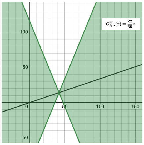
that is, generalized Cayley operator is ${\lambda }_C=\frac{17}{7}$-Lipschitz-continuous, where ${\lambda }_C=\frac{2+{\lambda }_{P_1}{r}_1}{r_1}=\frac{2+1.\frac{7}{5}}{\frac{7}{5}}=\frac{17}{7}$. Furthermore,

$$\begin{array}{cc}\hfill \parallel Y_{P_2,\rho }^N\left(x\right)-Y_{P_2,\rho }^N\left(y\right)\parallel & =∥\frac{267}{140}x-\frac{267}{140}y∥\hfill \\ \hfill & =\frac{267}{140}\parallel x-y\parallel \hfill \\ \hfill & \le \frac{22}{9}\parallel x-y\parallel ,\hfill \end{array}$$

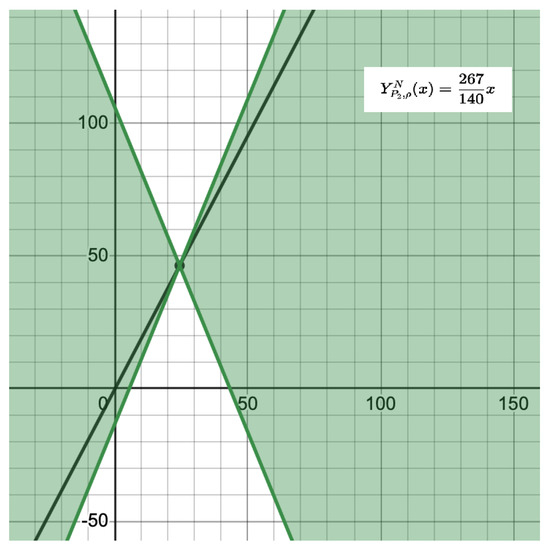
that is, the generalized Yosida approximation operator is ${\lambda }_Y=\frac{22}{9}$-Lipschitz-continuous, where ${\lambda }_Y=\frac{{\lambda }_{P_2}{r}_2+1}{\lambda r_2}=\frac{2·\frac{9}{4}+1}{1·\frac{9}{4}}=\frac{22}{9}$. Moreover,

$$\begin{array}{cc}\hfill \langle Y_{P_2,\rho }^M\left(x\right)-Y_{P_2,\rho }^M\left(y\right),x-y\rangle & =\langle \frac{267}{140}x-\frac{267}{140}y,x-y\rangle \hfill \\ \hfill & =\frac{267}{140}\langle x-y,x-y\rangle \hfill \\ \hfill & =\frac{267}{140}{\parallel x-y\parallel }^2\hfill \\ \hfill & \ge \frac{65}{36}{\parallel x-y\parallel }^2,\hfill \end{array}$$

that is, generalized Yosida approximation operator is ${\delta }_Y=\frac{65}{36}$-strongly accretive, where ${\delta }_Y=\frac{r_2^2-1}{\lambda r_2}=\frac{{\left(\frac{9}{4}\right)}^2-1}{1·\frac{9}{4}}=\frac{65}{36}$.

It is a well-known fact that for a Lipschitz-continuous function, there exists a double cone whose origin can be moved along the graph so that the whole graph always stays outside the double cone. The following figures (Figure 1 and Figure 2) demonstrate the Lipschitz continuity of generalized Cayley operator and generalized Yosida approximation operator calculated above, respectively.

6. Application

A dynamical system is a system that changes over time according to a set of fixed rules and determine how one state of the system moves to another state. On the other hand, a dynamical system describes the disequilibrium adjustment processes which may produce important transient phenomenon prior to the achievement of steady state. Dynamical system is a generalization of classical mechanics where the equation of motion postulated directly and are not constrained to be Euler–Lagrange equations of a least action principle.

Dynamical system theory has been applied in the field of neuroscience, cognitive development, equation of motion, electronic circuits, chaotic system (double pendulum), etc.

As an application of system of mixed variational inclusions involving the generalized Cayley operator and the generalized Yosida approximation operator (1), we mention a system of resolvent dynamical systems.

By using Lemma 3, we suggest the following system of resolvent dynamical systems:

$$\begin{array}{c}\frac{\mathrm{d}\left(A\left(x\right)\right)}{\mathrm{d}t}={\xi }_1\left[R_{P_1,\lambda }^M\left\{g\left(y\right)-\lambda C_{P_1,\lambda }^M\left(A\left(x\right)\right)\right\}-g\left(y\right)\right],x\left(t_0\right)=t_0\in \tilde{E}\mathrm{over}[t_0,\infty ),\\ \frac{\mathrm{d}\left(B\left(y\right)\right)}{\mathrm{d}t}={\xi }_2\left[R_{P_2,\rho }^N\left\{g\left(x\right)-\rho Y_{P_2,\rho }^N\left(B\left(y\right)\right)\right\}-g\left(x\right)\right],y\left(t_0\right)=t_0\in \tilde{E}\mathrm{over}[t_0,\infty ),\end{array}$$

(30)

where ${\xi }_1$ and ${\xi }_2$ are parameters.

It can be shown easily that by using the techniques of Noor [38], the Gronwall lemma and Lyapunov function, which are the trajectory of the solution of the system of resolvent dynamical systems (30), converge globally exponentially to the unique solution of system of mixed variational inclusions involving the generalized Cayley operator and the generalized Yosida approximation operator (1).

7. Conclusions

It is well known that the Cayley operator, the Yosida approximation operator, and a system of variational inclusions are application oriented. This paper is focused on the study of a system of mixed variational inclusions involving the generalized Cayley operator and the generalized Yosida approximation operator in q-uniformly smooth Banach space. We obtain the unique solution of our system, and we discuss the convergence criteria by suggesting an iterative algorithm. Two examples are provided with an application.

The novelty of work lies in the fact that our results are refinement of previously known results (see for example [8,9,13,18,26,28,33,36]).

Our results can be extended further and may be useful for other scientists.

References

- Baiocchi, C. Sur un problème à frontière libre traduisant le filtrage de liquides à travers des milieux poreux. C. R. Acad. Sci. Paris Sèr 1971, A-B 273, 1215–1217. [Google Scholar]
- Baiocchi, C.; Brezzi, F.; Comincioli, V. Free boundary problems in fluid flow through porous media. In Proceedings of the Second International Symposium on Finite Element Methods in Flow Problems, Santa Margharita, Italy, 14–18 June 1976; pp. 407–420. [Google Scholar]
- Brèzis, H.; Stampacchia, G. Sur la règularitè de la solution d’inèquations elliptiques. Bull. Soc. Math. France 1968, 96, 153–180. [Google Scholar] [CrossRef]
- Cryer, C.W. A bibliography of free boundary problems. Math. Res. Cent. Rep. 1977, 1793, 36. [Google Scholar]
- Cryer, C.W.; Fetter, H. The numerical solution of axisymmetric free boundary porous well problems using variational inequalities. Math. Res. Cent. Rep. 1977, 1761, 20–37. [Google Scholar]
- Hassouni, A.; Moudafi, A. A perturbed algorithm for variational inclusions. J. Math. Anal. Appl. 1994, 185, 706–712. [Google Scholar] [CrossRef]
- Fang, Y.P.; Huang, N.J. H-accretive operators and resolvent operator technique for solving variational inclusions in Banach spaces. Appl. Math. Lett. 2004, 17, 647–653. [Google Scholar] [CrossRef]
- Huang, N.J.; Fang, Y.P. Generalized m-accretive operators in Banach spaces. J. Sichaun Univ. 2001, 38, 591–592. [Google Scholar]
- Huang, N.J.; Fang, Y.P.; Cho, Y.J. Generalized m-accretive mappings and variational inclusions in Banch spaces. J. Concrete Appl. Math. 2005, 3, 31–40. [Google Scholar]
- Pang, J.S. Asymmetric variational inequality problems over product sets: Applications and iterative methods. Math. Program. 1985, 31, 206–219. [Google Scholar] [CrossRef]
- Cohen, G.; Chaplais, F. Nested monotony for variational inequalities over a product of spaces and convergence of iterative algorithms. J. Optim. Theory Appl. 1988, 59, 360–390. [Google Scholar] [CrossRef]
- Bianchi, M. Pseudo P-Monotone Operators and Variational Inequalities; Report 6; Istituto di Econometria e Mathematica per le Decisioni Economiche, Universita Cattolica del Sacro Cuore: Milan, Italy, 1993. [Google Scholar]
- Ansari, Q.H.; Yao, J.C. A fixed point theorem and its applications to a system of variational inequalities. Bull. Austral. Math. Soc. 1999, 59, 433–442. [Google Scholar] [CrossRef]
- Yan, W.Y.; Fang, Y.P.; Huang, N.J. A new system of set-valued variational inclusions with H-monotone operators. Math. Inequal. Appl. 2005, 8, 537–546. [Google Scholar] [CrossRef]
- Zou, Y.Z.; Huang, N.J. H(·,·)-accretive operator with an application for solving variational inclusions in Banach spaces. Appl. Math. Comput. 2008, 204, 809–816. [Google Scholar] [CrossRef]
- Chang, S.S. Set-valued variational inclusions in Banach spaces. J. Math. Anal. Appl. 2000, 248, 438–454. [Google Scholar] [CrossRef]
- Chang, S.S. Existence and approximation of solutions for set-valued variational inclusions in Banach spaces. Nonlinear Anal. 2001, 47, 583–594. [Google Scholar] [CrossRef]
- Ahmad, R.; Ansari, Q.H. An iterative algorithm for generalized nonlinear variational inclusions. Appl. Math. Lett. 2000, 13, 23–26. [Google Scholar] [CrossRef][Green Version]
- Ding, X.P. Perturbed proximal point algorithms for generalized quasi-variational inclusions. J. Math. Anal. Appl. 1997, 210, 88–101. [Google Scholar] [CrossRef]
- Alber, Y.; Yao, J.C. Algorithm for generalized multi-valued co-variational inequalities in Banach spaces. Funct. Diff. Equ. 2000, 7, 5–13. [Google Scholar]
- Ceng, L.C.; Latif, A.; Yao, J.C. On solutions of a system of variational inequalities and fixed point problems in Banach spaces. Fixed Point Theory Appl. 2013, 176, 1–34. [Google Scholar] [CrossRef]
- Ceng, L.C.; Wang, C.Y.; Yao, J.C. Strong convergence theorems by a relaxed extragradient method for a general system of variational inequalities. Math. Methods Oper. Res. 2008, 67, 375–390. [Google Scholar] [CrossRef]
- Ceng, L.C.; Plubtieng, S.; Wong, M.M.; Yao, J.C. System of variational inequalities with constraints of mixed equilibria, variational inequalities, and convex minimization and fixed point problems. J. Nonlinear Convex Anal. 2015, 16, 385–421. [Google Scholar]
- Ceng, L.C.; Guu, S.M.; Yao, J.C. Hybrid viscosity CQ method for finding a common solution of a variational inequality, a general system of variational inequalities, and a fixed point theorem. Fixed Point Theory Appl. 2013, 313, 1–25. [Google Scholar] [CrossRef]
- Qin, X.; Chang, S.S.; Cho, Y.J.; Kang, S.M. Approximation of solutions to a system of variational inclusions in Banach spaces. J. Inequal. Appl. 2010, 2010, 916806. [Google Scholar] [CrossRef]
- Ahmad, R.; Ahmad, I.; Rather, Z.A.; Wang, Y. Generalized complementarity problem with three classes of generalized variational inequalities involving XOR-operator. J. Math. 2021, 2021, 6629203. [Google Scholar]
- Ahmad, R.; Ali, I.; Li, X.B.; Ishtyak, M.; Wen, C.F. System of multi-valued mixed variational inclusions with XOR-operation in real ordered uniformly smooth Banach spaces. Mathematics 2019, 7, 1027. [Google Scholar] [CrossRef]
- Ahmad, I.; Yao, J.C.; Ahmad, R.; Ishtyak, M. System of Yosida inclusions involving XOR-operation. J. Nonlinear Convex Anal. 2017, 18, 831–845. [Google Scholar]
- De, A. Hille-Yosida Theorem and Some Applications. Ph.D. Thesis, Department of Mathematics and Its Applications, Central European University, Budapest, Hungary, 2015. [Google Scholar]
- Byrne, C.L. A unified treatment of some iterative algorithms in signal processing and image reconstruction. Inverse Probl. 2004, 20, 103–120. [Google Scholar] [CrossRef]
- Helmberg, G. Introduction to Spectral Theory in Hilbert Space: The Cayley Transform; North-Holland Series in Applied Mathematics and Mechanics, Applied Mathematics and Mechanics #6; North Holland Publishing Company: Amsterdam, The Netherlands, 1969. [Google Scholar]
- Cayley, A. Sur quelques propriétés des déterminants gauches. J. Reine Angew. Math. 1846, 32, 119–123. [Google Scholar]
- Iqbal, J.; Rajpoot, A.K.; Islam, M.; Ahmad, R.; Wang, Y. System of generalized variational inclusions involving Cayley operators and XOR-operation in q-uniformly smooth Banach spaces. Mathematics 2022, 10, 2837. [Google Scholar] [CrossRef]
- Althubiti, S.; Mennouni, A. A novel projection method for Cauchy-type systems of singular integro-differential equations. Mathematics 2022, 10, 2694. [Google Scholar] [CrossRef]
- Xu, H.K. Inequalities in Banach spaces with applications. Nonlinear Anal. 1991, 16, 1127–1138. [Google Scholar] [CrossRef]
- Ahmad, R.; Ali, I.; Rahaman, M.; Ishtyak, M. Cayley inclusion problem with its corresponding generalized resolvent equation problem in uniformly smooth Banach spaces. Appl. Anal. 2022, 101, 1354–1368. [Google Scholar] [CrossRef]
- Weng, X.L. Fixed point iteration for local strictly pseudo-contractive mapping. Proc. Am. Math. Soc. 1991, 13, 727–731. [Google Scholar] [CrossRef]
- Noor, M.A. Implicit resolvent dynamical systems for quasi variational inclusions. J. Math. Anal. Appl. 2002, 269, 216–226. [Google Scholar] [CrossRef]
Publisher’s Note: MDPI stays neutral with regard to jurisdictional claims in published maps and institutional affiliations. |
© 2022 by the authors. Licensee MDPI, Basel, Switzerland. This article is an open access article distributed under the terms and conditions of the Creative Commons Attribution (CC BY) license (https://creativecommons.org/licenses/by/4.0/).