Optimising Energy Management in Hybrid Microgrids

Abstract

This article deals with the optimization of the operation of hybrid microgrids. Both the problem of controlling the management of load sharing between the different generators and energy storage and possible solutions for the integration of the microgrid into the electricity market will be discussed. Solar and wind energy as well as hybrid storage with hydrogen, as renewable sources, will be considered, which allows management of the energy balance on different time scales. The Machine Learning method of Decision Trees, combined with ensemble methods, will also be introduced to study the optimization of microgrids. The conclusions obtained indicate that the development of suitable controllers can facilitate a competitive participation of renewable energies and the integration of microgrids in the electricity system.

1. Introduction

In recent years, the microgrid paradigm has emerged, introduced in the early 21st century by Lasseter [1] as an approach that considers generation and associated loads as a subsystem or microgrid. A microgrid can be considered as a set of loads, generators and storage that can be managed in isolation or connected to the rest of the grid in a coordinated manner to supply electricity reliably [2,3,4,5,6,7]. In emergency situations (faults, disturbances, etc.), the generators and the corresponding loads can be separated from the distribution grid, maintaining service without damaging the integrity of the system. Although originally associated with electricity grids, the concept has been broadened to any set of equipment, such as loads, storage systems and generators, which operates as a unique manageable system that can provide both electrical and thermal power or fuel to a given area [8]. Today, the operation of Distributed Energy Resources (DER) together with manageable loads (domestic consumption or electric vehicles) and various forms of storage such as batteries, supercapacitors or flywheels, is at the core of the hybrid microgrid concept [9]. A microgrid can operate interconnected to the utility through the main distribution grid, using the so-called Point of Common Coupling (PCC), or in island mode, and can also be interconnected with other microgrid systems, which can lead to more complex structures.

The management of hybrid microgrids presents many challenges [10,11], as they can operate either in island mode or connected to the main grid through the PCC. Proper management of the microgrid is, therefore, necessary for stable and economically efficient operation in both situations. The management system must control and adjust both frequency and voltage in either operating mode, share all the loads between the different Distributed Generators (DG) and storage, control the flow with the main grid and optimize operating costs. In grid-connected mode, voltage and frequency will be set by the main grid, which has synchronous generators and large rolling storage systems.

A necessary step in the difficult process of managing a hybrid microgrid is the mathematical modeling of the aspects (power flow, generation, storage, etc.) of that grid, for a next analysis with method. Several methods are, today, applying for this aim: optimizing energy management. Different methods and algorithms have been developed, and are developing [12,13], such as heuristic methods, optimization methods and Machine Learning methods, which will be predominant in the near future since they can compete in accuracy with the others, and because they can be adapted to different topologies, having enough data.

We present in this article a detailed and deep mathematical modeling development, which is not normally found in the bibliography, and is the basis of two heuristic methods (Hysteresis Band Control and control by means of Fuzzy Logic) and the Decision Trees Machine Learning method, combined with ensemble methods, concluding with a comparison of these methods in a microgrid.

This article is organized as follows: the next section presents the main challenges and functions of hybrid microgrids, along with some benefits that can be derived from their correct operation. Section 3 introduces energy management systems and their need to be modeled mathematically. Section 4 then mathematically models the main aspects of a hybrid microgrid to be taken into account when managing them, such as power flow equations, the generation of electrical energy, its storage, power converters, energy consumption and CO₂ emissions and other factors. In Section 5, the metaheuristic techniques are developed: they will be defined and their types will be classified according to the process they follow. The main ones (the Hysteresis Band Control and control by means of Fuzzy Logic) will be developed, although at the end of the chapter, mention will be made of some techniques that are either evolutions of other techniques or that are less well known but are widely used due to their good results. Section 6 introduces the Machine Learning method of Decision Trees, their basis, classification and some applications, to continue with the development of Decision Trees. In that section, bagging and boosting ensemble methods are also introduced. Section 7 details the design and experimental results obtained from the comparison operation of a laboratory microgrid. Section 8 discusses some of the open lines of research, and finally ends with the conclusions, where the two main ones are the mathematical modeling compiled in a single article, including hybrid components (renewable energy and storage), and that the Decision Tree method can be applied to the energy management of a hybrid microgrid, but without a great advantage over more classical methods such as Hysteresis Band Control or the application of Fuzzy Logic.

2. Management of Hybrid Microgrids

The objective of the management and control of a microgrid is to provide the energy demanded by the loads, using generation and storage systems efficiently and reliably, both under regular conditions and when contingencies occur, whether or not there is a connection to the external network.

Hybrid microgrids introduce a number of operational challenges that must be taken into account in the design of their management and protection systems, due to certain particularities that distinguish them from other systems. According to Olivares et al. [14], the most relevant are:

• Power flows. In contrast to conventional grids, the integration of DGs in low voltage can result in bi-directional power flows and lead to difficulties in protection systems or undesirable flow patterns.
• Stability. Local oscillations may occur as a result of the interaction of DG management systems and problematic transitions between stand-alone and grid-connected mode.
• Network model. The generally accepted assumptions of three balanced phases, inductive transmission lines and constant loads become meaningless in this type of network, leading to the need to adapt the models to the new situation. A hybrid microgrid is intrinsically subject to load unbalance by the DGs themselves.
• Low inertia. The dynamic characteristics of DG equipment, fundamentally those that are electronically coupled, are different from those based on large generation turbines. If appropriate monitoring and management measures are not implemented, the low inertia of the system can lead to considerable frequency deviations in the isolated mode of operation.
• Uncertainty. In hybrid microgrids there is greater uncertainty regarding demand and, above all, generation, as the use of renewable energies means that generation is linked to environmental conditions. Therefore, reliable and economic operation must take into account weather forecasting.

Under these circumstances, the management system must ensure reliable operation of the microgrid. The main functions that can be requested from the management system in the microgrid are [14,15,16]:

• Control of voltages and currents in the various DGs, according to the standards and adequately reducing oscillations.
• Frequency and voltage regulation in both stand-alone and grid-connected modes.
• Power balancing, when changes are produced in both generation and load, while maintaining voltage and frequency within acceptable limits.
• Demand Side Management (DSM) mechanisms that allow some fluctuation in the demand of a part of the loads to adapt to the requirements of the hybrid microgrid.
• Smooth transition between operating modes, using the most appropriate strategy for each of them and promptly identifying the situations that produce the switching. Resynchronization with the main network.
• Economic dispatch, distributing the load between the different DGs and storage systems in such a way as to reduce the cost of operation, while maintaining reliability. Optimization of the cost of operation will include maximizing the economic benefit in the case of grid connection.
• Management of power flows between the microgrid and the main network and, where appropriate, with other microgrids.

3. Energy Management System (EMS)

The architecture of a system is defined as the fundamental organization of a system, including its components, the relationships between them and the environment and the principles that govern its design and evolution [17,18]. Among the different control architectures, centralized, decentralized and distributed control architectures have been widely used in industry. On the one hand, the centralized implementation stands out for having greater precision, since the control of the process in question is carried out by a single controller, which receives all the signals provided by the network sensors and, after the control process, issues the values to be taken by the different actuators to achieve correct operation [19]. It is therefore a master–slave configuration in which the controller tries to optimize the operation of a set formed by all the subsystems of the network or process, leaving aside the interest that the subsystems themselves may have in optimizing their own operation at the expense of the common good. On the other hand, the decentralized implementation delegates the control problem to several controllers, reducing the computational expense, but also reducing the accuracy of the controller, as input/output data may overlap. Undoubtedly, the great benefit of this type of architecture lies in the ease of implementation with respect to centralized implementation, due to the reduction of a problem into multiple problems of less difficulty. Halfway between centralized and decentralized implementation is the distributed control architecture. In this architecture, there are problems that are related to each other, allowing the coordination of subsystems. This topology is characteristic of microgrids in which each subsystem has a control objective that is different from the others. The higher the number of components in the microgrid, the higher the data traffic between the different controllers and subsystems, thus requiring more bandwidth in the communication system. However, a distributed implementation can reduce data traffic compared to a centralized one, due to the reduced difficulty of the ‘local subproblems’ that make up the optimization problem.

A fundamental part of a microgrid is the control system, and more specifically, the control strategy or method that will manage the operation of the microgrid in terms of energy generation and demand, so that the energy storage and the external distribution network can satisfy, at all times, the energy balance in the system as a whole. The Energy Management System (EMS) is the system that performs this task, trying to achieve an efficient use of the different components of the microgrid [20,21]. In order to achieve this goal of efficient use, mathematical modeling of the parts of the system is essential.

4. Mathematical Modeling

4.1. Power Flow Equations

Each interconnecting component of an electrical network is called a branch or line and links a node n to another node m in the network. A line can be modeled by its single-phase equivalent circuit. This equivalent circuit accounts for the electrical properties of the conductors (conductivity and insulation) and the physical properties (diameter and distance between conductors). The most commonly used equivalent circuit of a line is the equivalent Π, although there are other models such as T. The complex admittance (inverse of impedance) values are represented by the letter Y together with an arbitrary number and each bus can have a generator connected to it at a voltage represented by the letter V + bus number.

Expressing the magnitudes in complex form, assuming a permanent and balanced sinusoidal regime, the system can be represented, in compact matrix notation, as follows:

$$I=Y_{BUS}V$$

(1)

where I is the column vector of currents at each node, V is the column vector of voltages at each node and Y_BUS is the admittance matrix. The admittance matrix is composed of complex numbers and has well-known properties: it is symmetrical, each element Y_nn of the diagonal is the sum of the admittances of the equivalent circuits Π that are connected to node n, and the off-diagonal elements Y_nm are the negative of the admittance of the equivalent Π connected between nodes n and m. Therefore, the admittance matrix is a square matrix of the same dimension as the number of buses. For each current n of the column vector, the power of bus n can be calculated as a factor of one, as follows:

$$s_n=\frac{V_n{I}_n^{\ast }}{S_{base}}=\frac{V_n}{S_{base}}{\left({\displaystyle \sum _{m=1}^N{Y}_{nm}{V}_m}\right)}^{\ast }=\frac{V_n}{S_{base}}{\displaystyle \sum _{m=1}^N{Y}_{nm}^{\ast }{V}_m^{\ast }}={\displaystyle \sum _{m=1}^N{v}_n{v}_m{e}^{j{\theta }_{nm}}\left(G_{nm}-j{B}_{nm}\right)},\hspace{0.33em}\hspace{0.33em}n=1,\dots ,N$$

(2)

where v_n is the modulus of V_n in per unit, θ_nm is the angle difference θ_n–θ_m, and Y_nm is the element nm of the admittance matrix G_nm + jB_nm also in per unit (pu). With Euler’s formula, one can write the above equation in rectangular coordinates in the complex plane as shown below:

$$s_n={\displaystyle \sum _{m=1}^N{v}_n{v}_m\left(\cos {\theta }_{nm}+j\sin {\theta }_{nm}\right)\left(G_{nm}-j{B}_{nm}\right)}\hspace{1em}n=1,\dots ,N$$

(3)

Remembering that the complex part of the apparent power is the reactive power and the real part is the active power, the two can be separated as follows:

$$\begin{array}{l}{p}_n={\displaystyle \sum _{m=1}^N{v}_n{v}_m\left(G_{nm}\cos {\theta }_{nm}+B_{nm}\sin {\theta }_{nm}\right)}\hspace{1em}n=1,\dots ,N\\ q_n={\displaystyle \sum _{m=1}^N{v}_n{v}_m\left(G_{nm}\sin {\theta }_{nm}-B_{nm}\cos {\theta }_{nm}\right)}\hspace{1em}n=1,\dots ,N\end{array}$$

(4)

The above representation is compact and allows observation of the asymmetric and non-linear character of the power flow equations, but to apply the relevant approximations and obtain a linearization, the special structure of the admittance matrix is considered: the elements of the diagonal Y_nn are the negative of the sum of the off-diagonal elements (negative of the admittance of the equivalent Π connected between nodes n and m) of the corresponding rows and of the shunt admittances of the bus (superscript sh). This can be seen in the three bus example below:

$$Y_{BUS}=\left(\begin{array}{ccc}{Y}_1^{sh}+Y_2+Y_8+Y_9^{sh}& -Y_2& -Y_8\\ -Y_2& Y_2+Y_3^{sh}+Y_5+Y_4^{sh}& -Y_5\\ -Y_8& -Y_5& Y_8+Y_7^{sh}+Y_5+Y_6^{sh}\end{array}\right)=\left(\begin{array}{ccc}{Y}_{11}& Y_{12}& Y_{13}\\ Y_{21}& Y_{22}& Y_{23}\\ Y_{31}& Y_{32}& Y_{33}\end{array}\right)$$

(5)

In the notation currently considered, with y_nm = y_mn, the admittance matrix is as follows:

$$Y_{BUS}=\left(\begin{array}{ccc}{y}_{12}^{sh}+y_{12}+y_{13}+y_{13}^{sh}& -y_{12}& -y_{13}\\ -y_{21}& y_{21}^{sh}+y_{21}+y_{23}+y_{23}^{sh}& -y_{23}\\ -y_{31}& -y_{32}& y_{31}^{sh}+y_{31}+y_{32}+y_{32}^{sh}\end{array}\right)$$

(6)

$$Y_{nm}=\left\{\begin{array}{cc}-y_{nm}& if m\ne n\\ {\displaystyle \sum _{m=1,m\ne n}^N{y}_{nm}+y_{nm}^{sh}}& if m=n\end{array}\right.$$

(7)

$${\displaystyle \sum _{m=1,m\ne n}^N{y}_{nm}+y_{nm}^{sh}}=y_n^{sh}+{\displaystyle \sum _{m=1,m\ne n}^N{g}_{nm}+j{b}_{nm}^{}}=j\left(b_n^{sh}+{\displaystyle \sum _{m=1,m\ne n}^N{b}_{nm}}\right)+g_n^{sh}{\displaystyle \sum _{m=1,m\ne n}^N{g}_{nm}}$$

(8)

Then, the active and reactive power equations for each node can be rewritten, based on the admittance of each line between bus n and bus m, Y_nm = −y_nm = −g_nm − jb_nm, and of the shunt of bus n as:

$$p_n=\left(g_n^{sh}+{\displaystyle \sum _{m=1,m\ne n}^N{g}_{nm}}\right)v_n^2-{\displaystyle \sum _{m=1,m\ne n}^N{v}_n{v}_m\left(g_{nm}\cos {\theta }_{nm}+b_{nm}\sin {\theta }_{nm}\right)}\hspace{1em}n=1,\dots ,N$$

(9)

$$q_n=-\left(b_n^{sh}+{\displaystyle \sum _{m=1,m\ne n}^N{b}_{nm}}\right)v_n^2-{\displaystyle \sum _{m=1,m\ne n}^N{v}_n{v}_m\left(g_{nm}\sin {\theta }_{nm}-b_{nm}\cos {\theta }_{nm}\right)}\hspace{1em}n=1,\dots ,N$$

(10)

You can group the summation terms, since the sum is over the same set, and take out common factor v_n in both equations by grouping the conductance and susceptance coefficients:

$$p_n=g_n^{sh}{v}_n^2+{\displaystyle \sum _{m=1,m\ne n}^N{g}_{nm}{v}_n\left(v_n-v_m\cos {\theta }_{nm}\right)-b_{nm}{v}_n{v}_m\sin {\theta }_{nm}}\hspace{1em}n=1,\dots ,N$$

(11)

$$q_n=-b_n^{sh}{v}_n^2+{\displaystyle \sum _{m=1,m\ne n}^N-b_{nm}{v}_n\left(v_n-v_m\cos {\theta }_{nm}\right)-g_{nm}{v}_n{v}_m\sin {\theta }_{nm}}\hspace{1em}n=1,\dots ,N$$

(12)

Different assumptions can now be made to linearize the power flow. Each approach assumes a different approach to the problem; however, the following assumptions are common according to the normal operation of an electrical power system [22,23]:

• The voltage values, expressed in per unit (pu), are very close to l.
• The difference between the angles of two interconnected buses is a small number close to 0.

Based on the above, to eliminate the non-linearity of the trigonometric functions, they are approximated by their Taylor series centered at zero and neglecting terms of order equal to or greater than three:

$$\cos {\theta }_{nm}\sim 1+\frac{{\theta }_{nm}^2}{2},\hspace{1em}\sin {\theta }_{nm}\sim {\theta }_{nm}$$

(13)

However, the quadratic term is non-linear and, in addition, there are products of several variables, which is also a non-linear function. The power equations at each bus n take the following form:

$$p_n=g_n^{sh}{v}_n^2+{\displaystyle \sum _{m=1,m\ne n}^N{g}_{nm}{v}_n\left(v_n-v_m-v_m\frac{{\theta }_{nm}^2}{2}\right)-b_{nm}{v}_n{v}_m{\theta }_{nm}}\hspace{1em}n=1,\dots ,N$$

(14)

$$q_n=-b_n^{sh}{v}_n^2+{\displaystyle \sum _{m=1,m\ne n}^N-b_{nm}{v}_n\left(v_n-v_m-v_m\frac{{\theta }_{nm}^2}{2}\right)-g_{nm}{v}_n{v}_m{\theta }_{nm}}\hspace{1em}n=1,\dots ,N$$

(15)

At this point, there is currently no consensus on the best approximation of the non-linear terms. Several approaches consider a second-order approximation based on the Taylor series of the products of two variables, which results in a linear form of the equations, except for the losses. In fact, power losses are non-convex quadratic functions which forces relaxations, such as piecewise linear function approximation or binary expansion, which give rise to a mixed integer linear programming problem (known by its acronym as MILP or MIP), or also convex relaxation, which generates a second-order conic programming problem; both are linear cases considering $v_n^2$ as a variable [24,25,26,27].

Since MIP-type problems are more costly to solve in terms of resources and time than continuous linear problems, other authors propose not considering the second order terms of the Taylor series expansion, both of the trigonometric functions and of the products of the variables, in such a way that the resulting flow is symmetric and allows calculating the voltage and angle value at each bus, as well as the powers, however in this approximation, losses are not represented [28].

Taking the first term of the trigonometric functions expansion, and according to Yang et al. [29], three linear approximations of the term v_n(v_n − v_m) are compared, being the one with the least error, in terms of voltage and active power flow, the one that considers a decomposition of the bus voltages as v_n = 1 + Δv_n, where Δv_n is an order of magnitude smaller than v_n, therefore:

$$v_n(v_n-v_m)=(1+\mathsf{\Delta }{v}_n)(\mathsf{\Delta }{v}_n-\mathsf{\Delta }{v}_m)=\mathsf{\Delta }{v}_n-\mathsf{\Delta }{v}_m+\mathsf{\Delta }{v}_n\mathsf{\Delta }{v}_n-\mathsf{\Delta }{v}_m\mathsf{\Delta }{v}_n\sim \mathsf{\Delta }{v}_n-\mathsf{\Delta }{v}_m$$

(16)

In the resulting product of the expansion, the multiplication of the difference of the voltages, Δv_nΔv_n, is neglected with respect to its nominal value of 1 pu, since the result is at most two orders of magnitude smaller than v_n; thus $v_n(v_n-v_m)\simeq v_n-v_m$. Furthermore, the voltage squared multiplying the shunt terms is simply approximated by the value of the voltage at that bus, and in the case of reactive power the shunt conductance is assumed to be negligible compared to the shunt susceptance. This gives rise to a linear problem in the voltage and angle variables [30,31].

Expanding the product terms of variables by their first order Taylor series gives the following:

$$\begin{array}{l}{v}_n{v}_m{\theta }_{nm}\simeq v_{n,0}{v}_{m,0}{\theta }_{nm}+\left(v_n{v}_m-v_{n,0}{v}_{m,0}\right){\theta }_{nm,0}={\theta }_{nm}\\ v_n{v}_m{\theta }_{nm}^2\simeq v_{n,0}{v}_{m,0}{\theta }_{nm}^2+\left(v_n{v}_m-v_{n,0}{v}_{m,0}\right){\theta }_{nm,0}^2={\theta }_{nm}^2\end{array}$$

(17)

where the subscript 0 denotes the point around which the expansion is performed, which in the case of the voltages is $v_{n,0}=v_{m,0}=1$, and in the case of the angle difference is ${\theta }_{nm,0}={\theta }_{nm,0}^2=0$, justified by the usual operating conditions in most power systems [23]. The power equations at each bus are then as follows

$$p_n=g_n^{sh}{v}_n^2+{\displaystyle \sum _{m=1,m\ne n}^N{g}_{nm}\left(v_n^2-v_n{v}_m-\frac{{\theta }_{nm}^2}{2}\right)-b_{nm}}{\theta }_{nm}$$

(18)

$$q_n=-b_n^{sh}{v}_n^2+{\displaystyle \sum _{m=1,m\ne n}^N-b_{nm}\left(v_n^2-v_n{v}_m-\frac{{\theta }_{nm}^2}{2}\right)-g_{nm}{\theta }_{nm}}$$

(19)

Neglecting $v_n{v}_m$ and ${\theta }_{nm}^2$, together with the approximation $v_n^2\simeq v_n$, the model of (29) is obtained, while taking the voltage squared as independent variable, the above equations can be rewritten, considering the following voltage product transformation:

$$v_n{v}_m=\frac{v_n^2+v_m^2}{2}-\frac{{\left(v_n-v_m\right)}^2}{2}$$

(20)

As

$$p_n=g_n^{sh}{v}_n^2+{\displaystyle \sum _{m=1,m\ne n}^N{g}_{nm}\left(\frac{v_n^2-v_m^2}{2}+\frac{{\left(v_n-v_m\right)}^2}{2}-\frac{{\theta }_{nm}^2}{2}\right)-b_{nm}}{\theta }_{nm}$$

(21)

$$q_n=-b_n^{sh}{v}_n^2+{\displaystyle \sum _{m=1,m\ne n}^N-b_{nm}\left(\frac{v_n^2-v_m^2}{2}+\frac{{\left(v_n-v_m\right)}^2}{2}-\frac{{\theta }_{nm}^2}{2}\right)-g_{nm}{\theta }_{nm}}$$

(22)

Approximating the terms with ${\theta }_{nm}^2$ and ${(v_n-v_m)}^2$, which account for the losses, by linear functions of ${\theta }_{nm}$ and $v_n^2-v_m^2$, we would now yield the method proposed by Yang et al. [32], which is linear with respect to the voltage squared and the angle value. However, rearranging the above expressions,

$$p_n=g_n^{sh}{v}_n^2+{\displaystyle \sum _{m=1,m\ne n}^N{g}_{nm}\frac{v_n^2-v_m^2}{2}-b_{nm}{\theta }_{nm}+g_{nm}\left(\frac{{\left(v_n-v_m\right)}^2}{2}-\frac{{\theta }_{nm}^2}{2}\right)}$$

(23)

$$q_n=-b_n^{sh}{v}_n^2+{\displaystyle \sum _{m=1,m\ne n}^N-b_{nm}\frac{v_n^2-v_m^2}{2}-g_{nm}{\theta }_{nm}-b_{nm}\left(\frac{{\left(v_n-v_m\right)}^2}{2}-\frac{{\theta }_{nm}^2}{2}\right)}$$

(24)

and considering the following approximation of ${(v_n-v_m)}^2/2$ around the point $v_n=v_m=1$

$$\frac{{\left(v_n-v_m\right)}^2}{2}\simeq \frac{1}{2}{\left[\left(v_n-v_m\right)\frac{v_n+v_m}{2}\right]}^2=\frac{{\left(v_n^2-v_m^2\right)}^2}{8}$$

(25)

the formulation of (26) is obtained:

$$p_n=g_n^{sh}{v}_n^2+{\displaystyle \sum _{m=1,m\ne n}^N{g}_{nm}\frac{v_n^2-v_m^2}{2}-b_{nm}{\theta }_{nm}+g_{nm}\left(\frac{{\left(v_n^2-v_m^2\right)}^2}{8}-\frac{{\theta }_{nm}^2}{2}\right)}$$

(26)

$$q_n=-b_n^{sh}{v}_n^2+{\displaystyle \sum _{m=1,m\ne n}^N-b_{nm}\frac{v_n^2-v_m^2}{2}-g_{nm}{\theta }_{nm}-b_{nm}\left(\frac{{\left(v_n^2-v_m^2\right)}^2}{8}-\frac{{\theta }_{nm}^2}{2}\right)}$$

(27)

In this case, given that the equations show the value of the angle difference ${\theta }_{nm}$ and its square ${\theta }_{nm}^2$, as well as the square of the squared voltage difference ${(v_n^2-v_m^2)}^2$, it is necessary to linearize these two terms by piecewise linear functions to properly estimate the losses.

At this point it is necessary to make a decision on the approximation of the power flow equations to be implemented in solving the problem. However, it requires two additional linearizations by piecewise functions, which makes it slower to solve than the simplified method of (30), which does not include terms that account for losses but is computationally faster since it only involves one linearization corresponding to the power limitation of the lines.

Since the objective of implementing these equations is to ensure the correct operation of the power system under study under different scenarios, the procedure involves the resolution of these flows in all cases, as the number of scenarios is very high, a more elaborate description results in possibly unaffordable computation times, which depends on the number of scenarios considered and the time intervals contained in each one.

In order not to limit the scenarios to be considered and the time steps, we implement the model evaluated by Yang et al. [29] and Morvaj et al. [33], originating from (30). As the case considered is a distribution network whose lines have a length of less than 5 km, without committing significant error, the shunt admittance of the lines can be considered null [34,35]. Naming v_nm = v_n − v_m, the linearized power flow equations are as shown below:

$$p_n=p_n^G-p_n^D={\displaystyle \sum _{m=1,m\ne n}^N{g}_{nm}{v}_{nm}-b_{nm}{\theta }_{nm}}={\displaystyle \sum _{m=1,m\ne n}^N{p}_{nm}}\hspace{1em}n=1,\dots ,N$$

(28)

$$q_n=q_n^G-q_n^D={\displaystyle \sum _{m=1,m\ne n}^N-b_{nm}{v}_{nm}-g_{nm}{\theta }_{nm}}={\displaystyle \sum _{m=1,m\ne n}^N{q}_{nm}}\hspace{1em}n=1,\dots ,N$$

(29)

where the superscripts denote power generation, G, and power demand, D. Each summand nm of the active and reactive power expressions is the power flow per each line linking bus n to bus m.

On the other hand, the maximum power constraint through the lines is defined by the inequality:

$$p_{nm}^2+q_{nm}^2\le s_{\max ,nm}^2=i_{\max ,nm}^2{v}_x^2\hspace{1em}\forall x=n,m$$

(30)

where S_max, is the maximum apparent power in per unit (pu) that can circulate through each line, i_max, is the maximum current that can pass through the conductor and v_x is the voltage at bus n or m. The manufacturers provide the maximum current limit because the limiting factor is the temperature of the conductor due to the heat caused by the passage of the current. The model of the conductors is given by the standards and technical requirements that can be found in the technical literature [36], and the value of the maximum current in [37,38], which is 285 A for underground conductors (20 °C ground temperature and 70 °C conductor temperature), and 262 A for overhead conductors (at 75 °C conductor temperature and 35 °C ambient temperature). This is what is known as the thermal limit of the conductors and is a factor to be considered in lines shorter than 80 km, as is the case; while between 80 and 320 km the limiting factor is the voltage drop, in lines longer than 320 km it is the stability of the angle [34]. The current limit depends on the conductor temperature, since the electrical parameters of the conductor vary with temperature, however, the change in these parameters would modify the power flow and therefore an iterative calculation would be necessary, in fact, this maximum current decreases with ambient temperature and the dynamics of heat transfer would have to be considered, which gives rise to a non-linear problem: the current limit of the conductors increases non-linearly with conductor temperature and decreases with ambient temperature [38]. This variation is not considered to be significant and the maximum current is assumed to be fixed and equal to that given above, at the given temperature.

4.2. Generation of Electrical Energy

The parameter representing the photovoltaic active power leaving the solar field and entering the inverter at each bus, in each scenario and time instant, is given by the following formula [39]:

$$P_{pv}(t)=P_{nom}\frac{G(t)}{G_n}\left[1-\alpha \left(T(t)+\frac{G(t)}{800}\left[NOCT-20\right]-25\right)\right]$$

(31)

where T is the ambient temperature, P_nom is the power at nominal conditions, G_n is the nominal irradiance in W/m² (this value is sometimes generalized to 1000 [40]), G is the incident irradiance in W/m², α is the parameter of the power-temperature characteristic in %/°C, NOCT takes the value of 45 °C and is the nominal operating temperature of the cell at 800 W/m² with 20 °C ambient temperature and 1 m/s wind. The alpha factor of the efficiency is negative, which implies an increase in efficiency with decreasing temperature. The inverter efficiency and other characteristics are introduced in more detail in later sections.

In the case of wind turbines, the parameter denoting the maximum energy extractable from the device is calculated using its power curve, but applying the inverter efficiency to the proportional part of the power flowing through the inverter:

$$P_{wt}^{\max }(t)=P_{wt}(t)(0.7+0.3{\eta }_{b2b}(t))\simeq P_{wt}(t)(0.7+0.3\cdot 0.965)=0.9895P_{wt}(t)$$

(32)

$$P_{wt}(t)=\left\{\begin{array}{cc}2100\left[1-e^{-{\left(\frac{c(t)}{5.692}\right)}^{3.398}}\right]& 2 \mathrm{m}/\mathrm{s}\le c(t)<20.5 \mathrm{m}/\mathrm{s}\\ 4378-111c(t)& 20.5 \mathrm{m}/\mathrm{s}\le c(t)\le 25 \mathrm{m}/\mathrm{s}\\ & \\ 0& \mathrm{any} \mathrm{other} \mathrm{case}\end{array}\right.$$

(33)

This gives the upper limits of active power injection to the grid, those of reactive power are related by means of the equations of the converters presented in the section corresponding to power converters.

4.3. Electrical Energy Storage

This section presents the equations that give the state of charge of each storage system on each bus, in each scenario and at each moment in time. The active and reactive power variables that appear represent the energy output/input of the system through the converter that connects the ESS (Energy Storage System) to the grid.

The following stochastic variables are defined for the load power, the discharge power and the state of charge of each ESS at each bus n for time t:

$$P_{in}^{ESS,n}(t)\hspace{0.33em},\hspace{0.33em}{P}_{out}^{ESS,n}(t)\hspace{0.33em},\hspace{0.33em}SOC(t)\hspace{0.33em}\ge 0$$

(34)

These powers are the real effective powers received or delivered by the ESSs, that is, they include the load and converter efficiency in their definition, which is explained in the following development.

The weight of the problem lies in the binary part, not in the linear part, therefore it is convenient to create a variable for loading and another for unloading and to use only a binary variable and its complementary to avoid simultaneous loading and unloading. This restriction is as follows:

$$P_{in}^{ESS,n}(t)\le b^{ESS,n}(t)P_{in,\max }^{ESS,n}\hspace{0.33em},\hspace{0.33em}{P}_{out}^{ESS,n}(t)\le (1-b^{ESS,n}(t))P_{out,\max }^{ESS,n}\hspace{0.33em}\hspace{1em}\forall ESS,n$$

(35)

where the subscript max denotes the nominal power of each storage system (ESS) on each bus n and the binary variable is b^ESS,n which takes the value 1 or 0 at each time t for each ESS on each bus n and each scenario. This constraint forces the load to zero if there is unloading and vice versa.

On the other hand, the load state model is estimated to be linear and without capacity reduction due to unloading depth or gradation. The correctness of this assumption is ensured by adding a number of constraints to limit the state of charge to a safe range of each ESS. The state of charge of each ESS on each bus n at each time t and scenario is given by the following expression:

$$SO{C}_{ESS,n}(t)=(1-\alpha \mathsf{\Delta }t)SO{C}_{ESS,n}(t-1)+P_{in}^{ESS,n}(t)\mathsf{\Delta }t-P_{out}^{ESS,n}(t)\mathsf{\Delta }t\hspace{1em}\forall ESS,n$$

(36)

where SOC represents the state of charge, the parameter α is the relative self-discharge per unit time and Δt is the time step. The upper limit of the state of charge of each ESS is defined by the following constraints:

$$SO{C}_{ESS,n}^{\max }DO{D}_{ESS,n}\le SO{C}_{ESS,n}(t)\le SO{C}_{ESS,n}^{\max }(1-DO{D}_{ESS,n})$$

(37)

where DOD is the relative depth of discharge parameter of each ESS on each bus, set to zero for flow batteries and 0.1 for lithium-ion batteries and hydrogen cells, as already introduced in the section on system components.

All these quantities are expressed in International System units, but to link these subsystems to the grid they must be expressed in per unit, and for this purpose they are simply redefined through the quotient between the base power. In addition, the definition of the charging and discharging power variables relate them to the converter that connects these systems to the grid and is where the charging and discharging efficiencies are applied, as well as those of each converter, as noted at the beginning:

$$p_{out}^{ESS,n}=\frac{P_{out}^{ESS,n}}{S_{base}}=\frac{p_{ESS2net,n}(t)}{{\eta }_{out}^{ESS,n}{\eta }_{conv}^{ESS,n}}\hspace{0.33em},\hspace{1em}{p}_{in}^{ESS,n}(t)=\frac{P_{in}^{ESS,n}(t)}{S_{base}}=p_{net2ESS,n}(t){\eta }_{in}^{ESS,n}{\eta }_{conv}^{ESS,n}$$

(38)

where conv refers to the power converters and the subscripts ESS2net indicate power transfer from the storage system to the grid and net2ESS from the grid to the storage system.

In the application case, the charging and discharging efficiencies are those justified in the system components section and the efficiency of the converters is approximated in a constant way based on the commercial model also chosen in the aforementioned section, with a value of 0.98.

Finally, constraints are necessary to force the initial SOC equal to the final SOC, during the time horizon, in order to increase the lifetime of the ESS. This variable, $SO{C}_{ESS,n}^0$, is not stochastic:

$$SO{C}_{ESS,n}(t_0)=SO{C}_{ESS,n}^0\hspace{0.33em},\hspace{1em}SO{C}_{ESS,n}(T)=SO{C}_{ESS,n}^0$$

(39)

4.4. Power Converters

One aspect to consider for power converters is their performance curve: PV plants and storage systems need to be able to deliver more than a certain percentage of the inverter’s rated power for the power output to be effective and work above the bend of the performance curve, whenever it is considered appropriate for them to inject power.

These curves describe a potential behavior and the three parameters that characterize them can be adjusted from a number of real samples or from the curve itself to obtain the continuous version. In other words, they are power functions that introduce non-linearities to the problem and must therefore be linearized. This approximation error is not remarkable since the performance reaches high values at relatively low powers. In this case, a discretization of the curve into four intervals is chosen. In order to model the active power output, parameters are created that represent the maximum power limit that can be generated at any given time by each system on each bus and in each scenario. These parameters are characterized by the super index max. Then, for example, the maximum PV active power produced at each time t is given by the following formula:

$$P_{pv}^{\max }(t)=\left\{\begin{array}{cc}{\eta }_1{P}_{pv}(t)& P_{pv}(t)\in [P_0,P_1]\\ {\eta }_2{P}_{pv}(t)& P_{pv}(t)\in (P_1,P_2]\\ {\eta }_3{P}_{pv}(t)& P_{pv}(t)\in (P_2,P_3]\\ ⋮& \\ {\eta }_u{P}_{pv}(t)& P_{pv}(t)\in (P_{u-1},P_u]\end{array}\right.=\left\{\begin{array}{cc}0.98P_{pv}(t)& 0.4\le P_{pv}(t)/P_{nom}\\ 0.972P_{pv}(t)& 0.2\le P_{pv}(t)/P_{nom}<0.4\\ 0.955P_{pv}(t)& 0.08\le P_{pv}(t)/P_{nom}<0.2\\ 0& \mathrm{any} \mathrm{other} \mathrm{case}\end{array}\right.$$

(40)

where Ppv(t) is the active power coming from the solar field at time t, η_n are the yields corresponding to the average of the discretized interval, P_nom is the nominal power of the inverter of the solar field and P_u, P_u−1 are the powers of each interval. This expression is applied to each PV system in each bus and scenario. In the specific case of the wind turbine with doubly fed induction machine (DFIG) this efficiency only applies to the percentage of the power that circulates through the converter, that is, about 30% of the generated power.

Another important component of these machines is the ability to absorb/inject reactive power. Based on the specific characteristics of each manufacturer’s model and for each application, the operating region of the converters is limited differently. In the case of PV inverters, the active power is limited to non-negative values so that the portion of the circle with the positive semi-axis of abscissa (right half of the circle) is obtained, in other words, the following constraints apply:

$$\begin{array}{l}\left[\sin \left(\frac{2\pi l}{k}\right)-\sin \left(\frac{2\pi (l-1)}{k}\right)\right]p_{pv}(t)-\left[\cos \left(\frac{2\pi l}{k}\right)-\cos \left(\frac{2\pi (l-1)}{k}\right)\right]q_{pv}(t)\le s_{inv}\sin \left(\frac{2\pi }{k}\right)\\ \\ \hspace{1em}\hspace{1em}0\le p_{pv}(t)\le P_{pv}^{\max }(t)/S_{base}\hspace{0.33em},\hspace{1em}-s_{inv}\le q_{pv}(t)\le s_{inv}\end{array}$$

(41)

where p_pv is the decision variable of active power per unit that the inverter or group of PV inverters deliver to the grid, q_pv is the variable of reactive power per unit that the PV inverter delivers to the grid and s_inv is the parameter corresponding to the nominal or maximum apparent power of the inverter also expressed in per unit (pu). Here s_inv is a deterministic parameter while p_pv and q_pv are stochastic variables. Again, the above expression is applied to each bus where there is a PV installation.

For wind turbines, the constraint is similar except that the power factor fp_wt, both inductive and capacitive, is limited to maximum values of 0.95, as indicated by the manufacturer [41]:

$$\begin{array}{l}\left[\sin \left(\frac{2\pi l}{k}\right)-\sin \left(\frac{2\pi (l-1)}{k}\right)\right]p_{wt}(t)-\left[\cos \left(\frac{2\pi l}{k}\right)-\cos \left(\frac{2\pi (l-1)}{k}\right)\right]q_{wt}(t)\le s_{wt}\sin \left(\frac{2\pi }{k}\right)\\ \\ \hspace{1em}\hspace{1em}0\le p_{wt}(t)\le P_{wt}^{}(t)/S_{base}\hspace{0.33em},\hspace{1em}-\tan ({\cos }^{-1}(f{p}_{wt}))s_{wt}\le q_{wt}(t)\le \tan ({\cos }^{-1}(f{p}_{wt}))s_{wt}\end{array}$$

(42)

The following consideration should be noted: inverters only provide/absorb reactive power from the grid if there is active power available in the solar field. Likewise, the DFIG only manages reactive power when it is possible to generate active power. In principle, this limitation is not due to the design of the inverters, but is normal practice in this type of installation. In algebraic terms, this is achieved by modifying the restriction of the reactive power limits. The photovoltaic case is shown as an example, but for all other converters it is analogous:

$$\left.\begin{array}{cc}-s_{inv}& P_{pv}^{\max }(t)>0\\ 0& P_{pv}^{\max }(t)=0\end{array}\right\}\le q_{pv}(t)\le \left\{\begin{array}{cc}{s}_{inv}& P_{pv}^{\max }(t)>0\\ 0& P_{pv}^{\max }(t)=0\end{array}\right.$$

(43)

The converters used in storage systems are a special case since the active power flow can be both positive and negative (discharge and load), however, the approach applied is to separate these two processes (to save binary variables and thus speed up the resolution) and apply a similar constraint to each one together with the additional reactive limitations presented by these converters:

$$\begin{array}{l}\left[\sin \left(\frac{2\pi l}{k}\right)-\sin \left(\frac{2\pi (l-1)}{k}\right)\right]p_{ESS2net}(t)-\left[\cos \left(\frac{2\pi l}{k}\right)-\cos \left(\frac{2\pi (l-1)}{k}\right)\right]q_{ESS}(t)\le s_{ESS}\sin \left(\frac{2\pi }{k}\right)\\ \left[\sin \left(\frac{2\pi l}{k}\right)-\sin \left(\frac{2\pi (l-1)}{k}\right)\right]p_{net2ESS}(t)-\left[\cos \left(\frac{2\pi l}{k}\right)-\cos \left(\frac{2\pi (l-1)}{k}\right)\right]q_{ESS}(t)\le s_{ESS}\sin \left(\frac{2\pi }{k}\right)\end{array}$$

(44)

where the subscript ESS2net indicates power transfer from the storage system to the grid and net2ESS from the grid to the storage system. These and the following constraints are for each ESS, at each bus, at each time and in each scenario. The capacitive (cap) and inductive (ind) reactive limits are defined by giving a range to the variable as follows:

$$-\sin ({\cos }^{-1}(f{p}_{ESS,ind}))s_{ESS}\le q_{ESS}(t)\le \sin ({\cos }^{-1}(f{p}_{ESS,cap}))s_{ESS}$$

(45)

where sESS is the nominal apparent power of the converter of each storage system.

In this way, the P-Q operating curve of these converters is approximated in such a way that there is a circle cut by a horizontal straight line at the top (capacitive power factor) and by another horizontal straight line at the bottom (inductive power factor). This approximation is conservative in the sense that it does not consider power peaks slightly above nominal, as these converters allow according to the manufacturer, nor does it represent the performance variation in a non-linear way in two quadrants: first and fourth. Note that these considerations could be added by combining circles that cut in such a way that the operating area is only that enclosed by all of them at the same time, however, this increases the computational time and it is not considered meaningful to implement this detail in this case.

The complete energy balance corresponding to the pu power generation can now be expressed as shown below:

$$p_n^G(t)=p_{wt}^n(t)+p_{pv}^n(t)+p_{ESS2net}^n(t)-p_{net2ESS}^n(t)$$

(46)

$$q_n^G(t)=q_{wt}^n(t)+q_{pv}^n(t)+q_{ESS2net}^n(t)-q_{net2ESS}^n(t)$$

(47)

Here all variables are expressed for each time point t, each bus n and stochastic scenario.

4.5. Energy Consumption

The consumption data are stochastic parameters as they vary over time, for each bus and each scenario. They are defined on the basis of the demand curve proposed in the literature [42,43], but modified to make it similar in shape to the Spanish typical curve. In turn, in the aforementioned literature, it is proposed that different loads depend on whether they correspond to the residential or industrial sector, and we have sought to maintain this distinction. The power factor of each bus is also known from the benchmark and the nominal power is given in its apparent form. The network demand is given as a percentage of the nominal power of each bus. Then, the active power to be supplied at each bus n is given by the following expression:

$$p_n^D(t)=\frac{1}{S_{base}}\left(S_{indus}(n)f{p}_{indus}(n)rat{e}_{indus}(t)+S_{res}(n)f{p}_{res}(n)rat{e}_{res}(t)\right)$$

(48)

where res denotes residential and indus denotes industrial, furthermore here S corresponds to the nominal apparent power of each bus. Equivalently, the reactive demand is constructed as follows:

$$q_n^D(t)=\frac{1}{S_{base}}\left(S_{indus}(n)\sqrt{1-f{p}_{indus}{(n)}^2}rat{e}_{indus}(t)+S_{res}(n)\sqrt{1-f{p}_{res}{(n)}^2}rat{e}_{res}(t)\right)$$

(49)

4.6. CO₂ Emissions and Other Factors

Finally, to define the objective function, it is necessary to estimate the CO₂ emissions corresponding to the import of energy from the transmission grid. This is achieved by applying a time-varying emissions factor that represents the number of metric tons of CO₂ that it costs to produce one MWh unit of energy. This factor is considered to be similar to the Spanish factor and depending on the case study will be constant over time or may vary. This factor is deterministic because there is no correlation with other variables and there are no studies of its prediction.

The CO₂ emissions corresponding to the import of energy from the slack bus over a period T are calculated using the following expression:

$$Emissions={\displaystyle \sum _t^T{f}_{C{O}_2}(t)p_{slack}(t)S_{base}\mathsf{\Delta }t}$$

(50)

The effect of this factor is studied in different sections. Note that the slack bus powers are free variables and if, for example, energy export is not allowed or the power factor is to be limited, constraints such as the following must be added:

$$p_{slack}(t)\ge 0\hspace{0.33em},\hspace{1em}{q}_{slack}(t)\ge 0$$

(51)

5. Heuristic Methods

Heuristic methods have been commonly used in the field of optimization, being able to obtain solutions quickly to complex problems that, even with the use of clusters of computers, may not have an optimal solution. To do so, they sacrifice solution accuracy at the cost of reduced computational cost and time. Nevertheless, they are capable of finding an exact solution to problems of relative simplicity.

These methods are often used in off-grids to find a suitable location for the development of this type of microgrids [44,45]. In recent years, research is being carried out on certain metaheuristic methods, such as Particle Swarm Optimization and Salp Swarm Algorithm, among others, which are population-based methods with promising results [46].

Heuristic methods are also applied, with success, to improve the effectiveness of the distribution network by means of reconfiguration. Reconfiguration of the distribution network aims to find the optimal combination of all switches in the distribution, mainly determining proper sizing and siting of DG together with network reconfiguration. In this way, some researchers, like Muhammad et al. [47], use the discrete network reconfiguration of the data set method, employing the Water Cycle Algorithm (WCA) together with dataset approach to reduce the complexity of search space. This type of method has good convergence performance, and can obtain a global optimal solution for single-objective optimization problems. Others, such as Helmi et al. [48], propose the Harris Hawks Optimization (HHO) to minimize the power losses of the network.

However, all heuristic methods that are inspired by natural processes have parameters that are highly dependent on their own algorithm; therefore, the algorithm may behave differently affecting its performance [49]. Furthermore, according to Yang, and in relation to computational cost, no consensus has been reached on what are the best values or configurations of an algorithm, nor on possible ways to adjust these parameters to achieve the best performance [50]. On the other hand, the selection of a method as the most appropriate for solving a problem such as energy management in hybrid microgrids is an open problem [51]. This is largely based on the “no free lunch” theorem [52] of mathematical optimization, which shows that at the same time that a heuristic is very efficient for one collection of problems, it is very inefficient for another collection.

So, there are a multitude of methods that can be applied in this field, without any of them being clearly better than any other for any topology and type of grid, as we have discussed in previous sections. Even though the optimal power flow is a non-convex problem [53], convex approximations for the power flow equations have been studied [54,55], but generally assuming strong approximations, such as all generators are constant current injections, which is far from real microgrids and further from hybrid microgrids [56].

In this paper, we try to optimize energy management without reconfiguring the network, assuming that the location and schedule of DG and storage banks does not depend on the utility, but on the consumers, and therefore, it is not in their hands to reconfigure the network. Thus, we will not take into account, for example, the temporary shifting of loads, which is currently possible with electric vehicles. The study of controllable loads could be attacked by stochastic optimization algorithms, according to Hosseini et al. [57] or Barbato et al. [58]. In the following, two heuristic methods known in the study of microgrids will be described, namely: Hysteresis Band Control and Fuzzy Logic Control.

5.1. Hysteresis Band Control

The heuristic method of Hysteresis Band Control has been a certain success in the field of microgrids. According to the example proposed by Ipsakis et al. [59], from which this control strategy will be explained, a hysteresis band consists of the operating range existing between two limit values of a problem variable, in this case, the State of Charge (SOC) or State of Charge of the accumulator. In this way, the storage units of the microgrid in the example, electrolyzer and fuel cell, absorb energy or give it up according to the band defined by the limit values mentioned:

• in case of lack of power, it will be the fuel cell that will give up power; and
• in case of reaching the maximum state of SOC, it will be the turn of the electrolyzer, which will start to operate at that moment of excess power.

This way of operating has benefits such as reducing the number of start-ups and shut-downs of the electrolyzer, which can reduce its life expectancy. Also, the example method achieves a protection of the accumulator by excluding it from excessively long operation.

Appropriate SOC limit values must be calculated to achieve effective control and in accordance with the operating requirements of the problem.

5.2. Control by Means of Fuzzy Logic

The Fuzzy Logic Control (FLC) method is characterized by reaching solutions to problems in which the data, variables, or in short, the available information, is ambiguous or imprecise, hence the term fuzzy. Therefore, fuzzy control is characterized by being described by what could be called discard logic, that is: If a certain event occurs, then the control signal will take the value ‘X’.

This is why Fuzzy Logic Control (FLC) lacks accuracy when it comes to providing robust solutions. However, Fuzzy Logic Control has some advantages that make it attractive for tackling certain types of problems, these are [60,61]:

• It provides an orderly and efficient working structure from information given orally and fuzzily by human experts.
• Due to its simplicity, it is easy to understand and simplifies the design of the problem, which gives it a quick implementation and a lower cost compared to other methods.
• It is capable of generating numerous output signals from any reasonable number of inputs.
• It does not require a model to find approximate solutions to the control problem and provides non-linear controllers.

We can brief the concept by explaining its methodology with the following steps: firstly, the input data provided are processed and a smearing or merging is performed on them. In this first step, certain qualitative characteristics are given a numerical value. Once this is done, decisions are made in accordance with logical relationships called Fuzzy Rules. Finally, the defuzzification process takes place, in which concrete data are obtained that will be used to generate the appropriate control signals required by the problem.

Despite the ease of implementation of the heuristic methods described above, the large number of restrictions and variables that appear in the microgrid under study make them a bad strategy to follow for its control, as it is difficult to find optimal solutions to the problem [62,63].

6. Machine Learning Methods

Machine Learning is a scientific discipline that tries to make systems learn automatically. Learning, in this context, means identifying complex patterns in millions of pieces of data [64,65]. The machine that actually learns is an algorithm that reviews the data and is able to predict future behavior in some fields of knowledge [66,67,68]. Machine Learning is therefore a process of knowledge induction, that is, a method of deriving a general statement by generalizing from statements describing particular cases.

Machine Learning is learning from data, it is discovering the structure and patterns underlying the data. The main objective of Machine Learning is to extract the information contained in a dataset to acquire knowledge to make decisions about new datasets [69]. Formally, and according to Mitchell [70], we can define the algorithms used by Machine Learning as:

“A computer program is said to learn from experience E with respect to some class of tasks T and performance measure P if its performance at tasks in T, as measured by P, improves with experience E”.

These learning algorithms are based on a set of data on which to learn and then apply the experience gained on other sets. It is necessary to evaluate its performance on a set other than the one on which the system has been trained in order to obtain a valid estimate of its generalizability to new examples. Thus, the available data set is divided into two subsets: on the one hand, we have the training set and, on the other one, the validation set or test set. In this way, the model is generated from the training data and evaluated in the test set, in which the accuracy of the model can be measured. The obtained result on this set is a good approximation to the expected one for the new data [71].

Therefore, generalization is one of the key aspects in the design of Machine Learning algorithms [72]. At the same time, the models must fit the training set and capture all its information. In this way, the problem of balancing bias and variance arises: bias measures the average error of the model using different training sets, while variance measures the sensitivity of the model to small changes in the training data [73]. In other words, very complex models have a low bias and a high variance, which is known as overfitting. On the other hand, simple models have a high bias but a very low variance. Overfitting occurs when, by adding levels to the Decision Tree, the hypotheses are so refined that they describe the examples used in the learning process very well; however, when evaluating the examples, an error occurs. That is, it classifies the training data very well, but then it fails to generalize the test set. This is because it learns down to the noise of the training set, adapting to the regularities of the training set [74]. Therefore, overfitting will be an important evaluation indicator to take into account in the study.

Machine Learning algorithms are usually divided into three categories, the first two being the most common:

• Supervised learning: this type of algorithm is based on prior learning, usually related to a system of labels associated with the data. This allows them to make decisions based on the previous data or even make predictions from these data. An example could be a spam detector, that is, a system that thinks it detects spam and labels an email as spam based on the patterns it has learned from the email history (keywords in the subject line, sender, text/image ratio, etc.).
• Unsupervised learning: unlike the previous type, these algorithms do not use prior knowledge. What they use is all the available data with the aim of finding patterns among them. If they find such patterns, they try to organize them in some way. For example, unsupervised learning is applied when you want to extract patterns from massive social media data, to recommend products or create advertising campaigns
• Reinforcement learning: in this less common case, an algorithm learns from its own experience. A trial-and-error process is normally used in which correct decisions are rewarded in some way (with reinforcement factors). In this way, the aim is to make the best decision in different situations. Examples include: DNA classifications, facial recognition, etc.

6.1. Operation with Machine Learning Models

The process to be followed for the construction of a Machine Learning system can be divided into:

1. Data collection. This is usually a tedious process that takes up a large part of the development of the system, since it is generally necessary to collect large amounts of data in order to ensure that the used sample is representative of the set under study.

2. Feature selection. This is a critical step since it is necessary to extract those variables that are useful to distinguish the patterns of each category.

3. Choice of model. In this step, we will choose the model that best fits our problem and that achieves the expected performance on the test set. This model, among other tasks, must maintain the bias-variance balance explained above.

4. Model training. In this phase, the classifier is built, whose parameters are adjusted from the training data set. Finding the parameters that fit our model is an optimization problem since the objective is always to minimize a certain objective function.

5. Evaluation of the model. Using the test set, an error measure is set and the performance of the model is obtained. If the result is not expected, it is necessary to test by going back to each of the previous points and go through the process again.

In mathematical terms, the principle of Machine Learning, in a supervised learning context, consists of starting from a sample of learning:

$$\mathcal{L}=\left\{(x_n,y_n)\left|n=1,2,\dots ,N\right.,x_n\in {\Re }^d,y_n\in \left\{1,2,\dots ,C\right\}\right\}$$

(52)

constituted by n realizations of a pair of random variables (X, Y), to construct a $f:{\Re }^d\to \left\{1,2,\dots ,C\right\}$ function which, given a new X input vector, can predict with some degree of certainty the variable $Y=f(X)$. For each observation (x_i, y_i) of $\mathcal{L}$, the variable $x_i\in X$ is called the input variable or explanatory variable and $y_i\in Y$ the dependent or output variable [75]. When the dependent variable is discrete or categorical, we speak about a classification problem; and when it is continuous, about a regression problem. That is to say, depending on the type of objects that we are trying to predict, there are two types of problems:

• Classification problems: They try to predict the classification of objects on a set of prefixed classes. For example, classifying whether a news is about sports, entertainment, politics, etc.
• Regression problems: They try to predict a real value. For example, predict the value of the stock market tomorrow from the stock market behavior that is stored (past).

One of the most widely used Machine Learning methods is Decision Tree Learning. This is a method for approximation of discrete-valued functions, robust to noisy data and able to learn disjoint expressions. There is a family of Decision Tree Learning algorithms: ID3, C4.5, … In turn, based on these Decision Trees, hybrid methods have been created that build more than one Decision Tree: Bagging, Boosting and Random Forest.

6.2. Decision Trees

Learning through Decision Trees is based on the principle of divide and conquer.

Let $\mathcal{L}$ a sample be defined as:

$$\mathcal{L}=\left\{(x_n,y_n)\left|n=1,2,\dots ,N\right.,x_n\in {\Re }^d,y_n\in \left\{1,2,\dots ,C\right\}\right\}$$

(53)

where N is the number of elements in the data set, C the number of distinct classes and d the number of variables defining the examples $x_n$ in the set. Each of these examples is represented by a vector $x_n$, which has its corresponding class label $y_n$ associated with it and it is defined by different variables, which can be numerical (their values are real numbers) or categorical (they take values in a finite set in which there is no ordering relationship). Sometimes, these vectors $x_n$ are also cited as feature vectors.

A T Decision Tree is an ordered sequence of decisions, normally from questions, in which the next decision depends on the answer to the current one. These decisions are taken normally from questions that are formulated on the variables that define each x element in order to assign them a y certain class. This process, including its corresponding questions, decisions and bifurcations, is naturally represented by means of a tree.

In a Decision Tree, each node of the tree is an attribute (field) of the examples, and each branch represents a possible value of that attribute. The first node is known as the root node, which is successively connected to the other nodes until it reaches the leaf nodes, those that have no descendants, that is, the end of the branches of the tree. Each node is assigned one of the questions of the sequence, while each leaf node is assigned a class label.

In this way, the question of the root node is asked of the whole set $\mathcal{L}$, which is subdivided until reaching the last nodes (leaves), which constitute a disjoint partition of the initial feature space. This happens because, when given a node, one and only one branch will be followed by each instance of the training set.

Decision Trees perform well with large volumes of data, as it does not require loading all data into memory at once. The computation time scales well with a linearly increasing number of columns [76].

The advantages of Decision Trees are that they are easy to understand and interpret, rule generation is simple, it reduces the complexity of the problem, and training time is not very long.

One of the disadvantages is that if an error is made at a high level, successive nodes would be poorly created. In the construction of a Decision Tree, the most complicated step is to determine which attribute to base a node on, because if there are many features, the algorithm would have many options for the training data, and it would be difficult to construct a Decision Tree.

However, Decision Trees can give good results if they are combined with ensemble methods. With these methods, instead of learning a single model, several models are learned, and the estimates from each model are combined.

Ensemble methods are combinations of models. In these techniques, it is necessary both to define how different models are to be created and how the results of each model will be combined to generate the final prediction. The aim of ensemble methods is to produce a better prediction than individual models (individual members of the ensemble).

The most common ensemble methods are Bagging, Boosting and Random Forest. In all of these methods, the training set is manipulated, but in each case with a different strategy [77].

In Bagging, different samples are extracted from the training set (bootstrap samples), and these bootstrap samples are used as if they were the true training set. Boosting, on the other hand, always works with the full data set, that is, the complete dataset is always used. In Boosting, we can manipulate the weights of the data in the training set to generate different models. At each iteration, Boosting learns a model that minimizes the sum of the weights of the misclassified data.

Finally, Breiman [78] presented an ensemble method called Random Forest where bagging is used together with a random selection of attributes. At each node of each tree in the forest, a subset of the available attributes at that node is randomly selected and the best of them is selected according to the splitting criteria used in the base algorithm. The number of randomly selected attributes is an input parameter.

7. Results

We have evaluated the following of the proposed models explained in the previous sections, in order to measure the accuracy: Hysteresis Band Control, Fuzzy Logic Control, and Decision Trees (DT). We propose the IEEE microgrid test system of 69-bus [79]. The 69-bus distribution network has a nominal voltage of 12.66 kV. Its base apparent power is 10 MVA. This system has 69 nodes and 73 branches, including tie-lines, as shown in Figure 1. The order of each branch is assumed to be that of the furthest node minus one unit, except for the tie-lines in the base scheme which run from 69 to 73. Thus, a total of 73 remote switches are installed in the network, 68 of which are sectioned and ready for possible reconfiguration. As mentioned, and described by Lan et al. [80], two wind units, two solar panels and some switches are located in the microgrid, and a battery storage unit is also installed in the hybrid microgrid. We have followed the same location:

In this article, we only show a first approximation of the methods to verify their viability and check primary results. In addition to achieving adequate energy management using all the tested models, regardless of the calculation time or the power and dedication of the used computers, we can highlight that for loads without large hourly differences (as it would have been the case for valley and peak periods with a large difference in the power value), the system can be controlled by applying the aforementioned modeling.

From the test results, it can be found the Machine Learning model (Decision Tree) can also recognize the states accurately for distribution systems, as we show in

Table 1. Root Medium Square Error (RMSE) (voltage of the network) with different models applied to the IEE 69-bus distribution network.

	RMSE
HBC	0.1781
FL	0.1563
DT	0.1471

HBC = Hysteresis Band Control; FL = Fuzzy Logic; DT = Decision Tree.

. We used the root medium square error for the comparison.

As we can see, the three tested methods have enough viability, taking into account the characteristics of the network. We cannot conclude a better performance for the Decision Tree-based model, because, although its result is better than the others, the test is based in a single evaluation and more evaluations with different cases (for example, with different cases of distribution of solar and wind generation and different loads) should be done in the future.

In the case of the most modern method, Decision Trees, it should be noted that both solar and wind generation have followed generation patterns established in advance, according to the data of Lan et al. [80]. Obviously, in an analysis with a real system, these future generation data should be based on historical data and take forecasting into account. In Machine Learning methods, the reliability of data and predictions is very important, as they are the foundation of this type of modeling; therefore, it is advisable to use more than one database, which will usually reduce the error of calculation and analysis. These used patterns have been the same for any unit of the same generation type; that is, all solar units follow the same pattern, and all wind units follow the same pattern. This has been done to simplify the performed analysis and in accordance with Kovousi–Fard and Khodei [81].

The evaluations are based on the values shown in Figure 2 (base case), which represents the total energy consumption over a standard day.

Figure 3 shows the values obtained in the energy storage units, including the battery allocated at node 15. It presents the 24-h values of the state of the charge (SOC) of all the devices (that is, those related to the PV systems and the aforementioned battery unit). As can be seen, the energy storage units are strongly influenced by the solar behavior and are discharged from 16–17 h onwards, as the PV power generated gradually decreases.

Figure 4 and Figure 5 show the two main cases studied: Figure 4 corresponds to the situation where there is no distributed generation, and Figure 5 where there is distributed generation. As can be seen in Figure 4, the voltage profile has been improved with the use of the three methods, not being able to conclude which of the three is the best, mainly because, although the three improve the initial case, depending on the section of the system to be analyzed, the best method is one or the other. The tie-switch distributions generated by each method are shown in

Table 2. Case without distributed generation: tie-switches of the configuration of the system.

	Initial	HBC	FL	DT
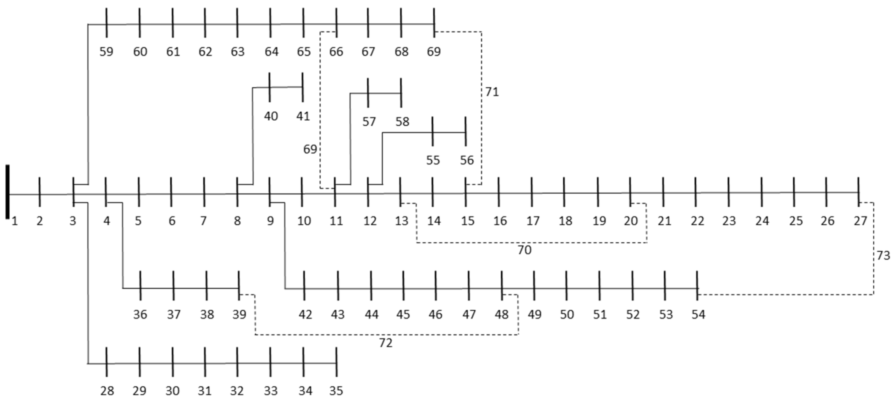
Tie-switches	69, 70, 71, 72, 73	14, 55, 61, 69, 70	13, 57, 61, 69, 70	13, 57, 61, 69, 70

HBC = Hysteresis Band Control; FL = Fuzzy Logic; DT = Decision Tree.

.

The IEEE-69 system has also been tested with distributed generation. As mentioned above, the distributions of wind and solar generation have followed the one published in the literature references, but

Table 3. Case with distributed generation: tie-switches of the configuration of the system and power (node–kW).

	Initial	HBC	FL	DT
Tie-switches	69, 70, 71, 72, 73	13, 55, 64, 69, 70	13, 58, 64, 69, 70	13, 58, 64, 69, 70
P (kW)	6–27.52	6–27.52	6–27.52	6–27.52
	25–30.45	25–30.45	25–30.45	25–30.45
	50–30.45	50–30.45	50–30.45	50–30.45
	68–342.05	68–342.05	68–342.05	68–342.05

HBC = Hysteresis Band Control; FL = Fuzzy Logic; DT = Decision Tree.

shows the averages of a typical day for the four nodes where they are located (6 and 68 for wind generation, and 25 and 50 for solar generation). In addition, Table 3 shows the tie-switches for each method. It can be seen in Figure 5 how, in general, the three methods improve the voltage profile of the system again after the reconfiguration of the system, being slightly different the solution (topology) found by each of them.

8. Conclusions

In this article, we presented the optimization of the operation of electrical hybrid microgrids, focused particularly on the mathematical modeling. The set of loads (consume), generators (with a predominance of the renewable energies) and storage systems (at the present, particularly batteries) makes up the electrical hybrid microgrid. The management of this type of networks presents many challenges and various options to be implemented.

The mathematical modeling of the different components is a very important step in the control and management that, in recent years, is increasing with the irruption into the market of new technologies or new models for the use of energy. The main contribution is the mathematical modeling of several components of the hybrid microgrid. This modeling can be used in different methods of control and management of the network, and its feasibility has been shown in three methods, including one based on the Decision Tree method, which belongs to the Machine Learning family. The results on a test system of 69 buses show that its implementation is possible.

The three methods have been compared both in the case of existence of distributed generation and in the case of its non-existence, in order to obtain a better view of their behavior. The three methods improve the voltage profile of the system, using a different topology, although similar (the tie-switches used are topologically very close or even the same), demonstrating their effectiveness. The integration of distributed generation in the system causes small differences in the results of each method, these differences being more noticeable the longer the line (or branch) in the system.

Nevertheless, although the results indicate that the Decision Trees method is partially better than other algorithms, more tests are needed and they need to be carried out with different typologies, not only of the network itself but also of its components. As a future research line, further tests with different generation and load levels can be identified.

References

- Lasseter, R.H. Microgrids. In Proceedings of the 2002 IEEE Power Engineering Society Winter Meeting (Conference Proceedings (Cat. No.02CH37309)), New York, NY, USA, 27–31 January 2002; pp. 305–308. [Google Scholar]
- Piagi, P.; Lasseter, R.H. Autonomous Control of Microgrids. In Proceedings of the 2006 IEEE Power Engineering Society General Meeting, Montreal, QC, Canada, 18–22 June 2006; p. 8. [Google Scholar] [CrossRef]
- Lopes, J.; Moreira, C.; Madureira, A. Defining Control Strategies for Microgrids Islanded Operation. IEEE Trans. Power Syst. 2006, 21, 916–924. [Google Scholar] [CrossRef] [Green Version]
- Baghaee, H.R. Real-Time Verification of New Controller to Improve Small/Large-Signal Stability and Fault Ride-Through Capability of Multi-DER Microgrids. IET Gener. Transm. Distrib. 2016, 10, 3068–3084. [Google Scholar] [CrossRef]
- Hirsch, A.; Parag, Y.; Guerrero, J. Microgrids: A Review of Technologies Key Drivers and Outstanding Issues. Renew. Sustain. Energy Rev. 2018, 90, 402–411. [Google Scholar] [CrossRef]
- Farrokhabadi, M.; Cañizares, C.A.; Simpson-Porco, J.W.; Nasr, E.; Fan, L. Microgrid Stability Definitions, Analysis, and Examples. IEEE Trans. Power Syst. 2019, 35, 13–29. [Google Scholar] [CrossRef]
- Ullah, S.; Khan, L.; Jamil, M.; Jafar, M.; Mumtaz, S.; Ahmad, S. A Finite-Time Robust Distributed Cooperative Secondary Control Protocol for Droop-Based Islanded AC Microgrids. Energies 2021, 14, 2936. [Google Scholar] [CrossRef]
- Moazeni, F.; Khazaei, J. Optimal Operation of Water-Energy Microgrids; A Mixed Integer Linear Programming Formulation. J. Clean. Prod. 2020, 275, 122776. [Google Scholar] [CrossRef]
- Bidram, A.; Lewis, F.L.; Davoudi, A. Distributed Control Systems for Small-Scale Power Networks: Using Multiagent Cooperative Control Theory. IEEE Control Syst. Mag. 2014, 34, 56–77. [Google Scholar] [CrossRef]
- Majumder, R. A Hybrid Microgrid with DC Connection at Back to Back Converters. IEEE Trans. Smart Grid 2014, 5, 251–259. [Google Scholar] [CrossRef]
- Tabar, V.S.; Ghassemzadeh, S.; Tohidi, S. Energy Management in Hybrid Microgrid with Considering Multiple Power Market and Real Time Demand Response. Energy 2019, 174, 10–23. [Google Scholar] [CrossRef]
- Minchala-Avila, L.I.; Garza-Castañón, L.E.; Vargas-Martín, A.; Zhang, Y. A Review of Optimal Control Techniques Applied to the Energy Management and Control of Microgrids. Procedia Comput. Sci. 2015, 52, 780–787. [Google Scholar] [CrossRef] [Green Version]
- Gómez Sánchez, M.; Macia, Y.M.; Fernández Gil, A.; Castro, C.; Nuñez González, S.M.; Pedrera Yanes, J. A Mathematical Model for the Optimization of Renewable Energy Systems. Mathematics 2021, 9, 39. [Google Scholar] [CrossRef]
- Olivares, D.E.; Mehrizi-Sani, A.; Etemadi, A.H.; Canizares, C.A.; Iravani, R.; Kazerani, M.; Hajimiragha, A.H.; Gomis-Bellmunt, O.; Saeedifard, A.; Palma-Behnke, R.; et al. Trends in Microgrid Control. IEEE Trans. Smart Grid 2014, 5, 1905–1919. [Google Scholar] [CrossRef]
- Nguyen, T.-L.; Guillo-Sansano, E.; Syed, M.H.; Nguyen, V.-H.; Blair, S.M.; Reguera, L.; Tran, Q.-T.; Caire, R.; Burt, G.M.; Gavriluta, C.; et al. Multi-Agent System with Plug and Play Feature for Distributed Secondary Control in Microgrid—Controller and Power Hardware-in-the-Loop Implementation. Energies 2018, 11, 3253. [Google Scholar] [CrossRef] [Green Version]
- Bazmohammadi, N.; Anvari-Moghaddam, A.; Tahsiri, A.; Madary, A.; Vasquez, J.C.; Guerrero, J.M. Stochastic Predictive Energy Management of Multi-Microgrid Systems. Appl. Sci. 2020, 10, 4833. [Google Scholar] [CrossRef]
- Díaz, N.L.; Vasquez, J.C.; Guerrero, J.M. A Communication-Less Distributed Control Architecture for Islanded Microgrids with Renewable Generation and Storage. IEEE Trans. Power Electron. 2018, 33, 1922–1939. [Google Scholar] [CrossRef] [Green Version]
- Lin, P.; Jin, C.; Xiao, J.; Li, X.; Shi, D.; Tang, Y.; Wang, P. A Distributed Control Architecture for Global System Economic Operation in Autonomous Hybrid AC/DC Microgrids. IEEE Trans. Smart Grid 2019, 10, 2603–2617. [Google Scholar] [CrossRef]
- Llaria, A.; Terrasson, G.; Curea, O.; Jiménez, J. Application of Wireless Sensor and Actuator Networks to Achieve Intelligent Microgrids: A Promising Approach towards a Global Smart Grid Deployment. Appl. Sci. 2016, 6, 61. [Google Scholar] [CrossRef] [Green Version]
- Chen, C.; Duan, S.; Cai, T.; Liu, B.; Hu, G. Smart energy management system for optimal microgrid economic operation. IET Renew. Power Gener. 2011, 5, 258–267. [Google Scholar] [CrossRef]
- Ahmad, A.; Khan, A.; Javaid, N.; Hussain, H.M.; Abdul, W.; Almogren, A.; Alamri, A.; Azim Niaz, I. An Optimized Home Energy Management System with Integrated Renewable Energy and Storage Resources. Energies 2017, 10, 549. [Google Scholar] [CrossRef] [Green Version]
- Bergen, A.R.; Vittal, V. Power Systems Analysis, 2nd ed.; Pearson: Upper Saddle River, NJ, USA, 2000. [Google Scholar]
- Nagrath, I.; Kothari, D. Modern Power System Analysis; McGraw-Hill: New Delhi, India, 1982. [Google Scholar]
- Akbari, T.; Bina, M.T. Linear Approximated Formulation of AC Optimal Power Flow Using Binary Discretisation. IET Gener. Transm. Distrib. 2016, 10, 1117–1123. [Google Scholar] [CrossRef] [Green Version]
- Zhang, H.; Vittal, V.; Heydt, G.; Quintero, J. A Relaxed AC Optimal Power Flow Model Based on a Taylor Series. In Proceedings of the 2013 IEEE Innovative Smart Grid Technologies-Asia (ISGT Asia), Bangalore, India, 10–13 November 2013. [Google Scholar] [CrossRef]
- Yang, Z.; Zhong, H.; Xia, Q.; Kang, C. A Novel Network Model for Optimal Power Flow with Reactive Power and Network Losses. Electr. Power Syst. Res. 2017, 144, 63–71. [Google Scholar] [CrossRef]
- Akbari, T.; Bina, M.T. A Linearized Formulation of AC Multi-Year Transmission Expansion Planning: A Mixed-Integer Linear Programming Approach. Electr. Power Syst. Res. 2014, 114, 93–100. [Google Scholar] [CrossRef]
- Attarha, A.; Amjady, N.; Conejo, A.J. Adaptive Robust AC Optimal Power Flow Considering Load and Wind Power Uncertainties. Int. J. Electr. Power Energy Syst. 2018, 96, 132–142. [Google Scholar] [CrossRef]
- Yang, J.; Zhang, N.; Kang, C.; Xia, Q. A State-Independent Linear Power Flow Model with Accurate Estimation of Voltage Magnitude. Trans. Power Syst. 2017, 32, 5. [Google Scholar] [CrossRef]
- Koster, A.M.C.A.; Lemkens, S. Designing AC Power Grids Using Integer Linear Programming. In INOC 2011, Lecture Notes in Computer Science; Pahl, J., Reiners, T., Voß, S., Eds.; Springer: Berlin/Heidelberg, Germany, 2011; Volume 6701, pp. 478–483. [Google Scholar] [CrossRef]
- Taylor, J.; Hover, F. Linear Relaxations for Transmission System Planning. IEEE Trans. Power Syst. 2011, 26, 4, 2533–2538. [Google Scholar] [CrossRef] [Green Version]
- Yang, Z.; Zhong, H.; Bose, A.; Zheng, T.; Xia, Q.; Kang, C. A Linearized OPF Model with Reactive Power and Voltage Magnitude: A Pathway to Improve the MW-Only DC OPF. IEEE Trans. Power Syst. 2018, 33, 2, 1734–1745. [Google Scholar] [CrossRef]
- Morvaj, B.; Evins, R.; Carmeliet, J. Optimization Framework for Distributed Energy Systems with Integrated Electrical Grid Constraints. Appl. Energy 2016, 171, 296–313. [Google Scholar] [CrossRef]
- Kothari, D.P. Power System Optimization. In Proceedings of the 2012 2nd National Conference on Computational Intelligence and Signal Processing (CISP), Guwahati, India, 2–3 March 2012; pp. 18–21. [Google Scholar] [CrossRef]
- Patel, N.; Porwal, D.; Bhoi, A.K.; Kothari, D.P.; Kalam, A. An Overview on Structural Advancements in Conventional Power System with Renewable Energy Integration and Role of Smart Grids in Future Power Corridors. In Green Energy and Technology; Bhoi, A., Sherpa, K., Kalam, A., Chae, G.S., Eds.; Springer: Singapore, 2020; pp. 1–15. [Google Scholar]
- Barsali, S. Benchmark Systems for Network Integration of Renewable and Distributed Energy Resources; Technical Brochure, TF C6.04.02; CIGRE: Paris, France, 2014. [Google Scholar]
- Rocha, R.C.C.; Berredo, R.C.; Bernis, R.A.O.; Gomes, E.M.; Nishimura, F.; Cicarelli, L.D.; Soares, M.R. New Technologies, Standards, and Maintenance Methods in Spacer Cable Systems. IEEE Trans. Power Deliv. 2002, 17, 2, 562–568. [Google Scholar] [CrossRef]
- Van den Brom, H.E.; van Leeuwen, R.; Rietveld, G.; Houtzager, E. Voltage Dependence of the Reference System in Medium- and High-Voltage Current Transformer Calibrations. IEEE Trans. Instrum. Meas. 2021, 70, 1502908. [Google Scholar] [CrossRef]
- Pantic, L.S.; Pavlović, T.M.; Milosavljević, D.D.; Radonjic, I.S.; Radovic, M.K.; Sazhko, G. The Assessment of Different Models to Predict Solar Module Temperature, Output Power and Efficiency for Nis, Serbia. Energy 2016, 109, 38–48. [Google Scholar] [CrossRef]
- Sun, V.; Asanakham, A.; Deethayat, T.; Kiatsiriroat, T. A New Method for Evaluating Nominal Operating Cell Temperature (NOCT) of Unglazed Photovoltaic Thermal Module. Energy Rep. 2020, 6, 1029–1042. [Google Scholar] [CrossRef]
- DFIG 2.1 MW—114. 2021. Available online: https://www.siemensgamesa.com/en-int/products-and-services/onshore/wind-turbine-sg-2-1-114 (accessed on 29 September 2021).
- Bilbao, J.; Torres, E.; Saenz, J. Load Curve Estimation by Means of Prediction Intervals. In Proceedings of the 2000 10th Mediterranean Electrotechnical Conference. Information Technology and Electrotechnology for the Mediterranean Countries. Proceedings. MeleCon 2000 (Cat. No.00CH37099), Lemesos, Cyprus, 29–31 May 2000; Volume 3, pp. 970–972. [Google Scholar] [CrossRef]
- Grandjean, A.; Adnot, J.; Binet, G. A Review and an Analysis of the Residential Electric Load Curve Models. Renew. Sustain. Energy Rev. 2012, 16, 9, 6539–6565. [Google Scholar] [CrossRef]
- Ranaboldo, M.; Ferrer-Martí, L.; García-Villoria, A.; Pastor Moreno, R. Heuristic Indicators for the Design of Community Off-Grid Electrification Systems Based on Multiple Renewable Energies. Energy 2013, 50, 501–512. [Google Scholar] [CrossRef]
- Borghei, M.; Ghassemi, M. Optimal Planning of Microgrids for Resilient Distribution Networks. Int. J. Electr. Power Energy Syst. 2021, 128, 106682. [Google Scholar] [CrossRef]
- Devarapalli, R.; Sinha, N.K.; Rao, B.V.; Knypinski, Ł.; Lakshmi, N.J.N.; García Márquez, F.P. Allocation of Real Power Generation Based on Computing over All Generation Cost: An Approach of Salp Swarm Algorithm. Arch. Electr. Eng. 2021, 70, 2, 337–349. [Google Scholar] [CrossRef]
- Muhammad, M.; Mokhlis, H.; Naidu, K.; Amin, A.; Franco, F.; Othman, M. Distribution Network Planning Enhancement via Network Reconfiguration and DG Integration Using Dataset Approach and Water Cycle Algorithm. J. Mod. Power Syst. Clean Energy 2020, 8, 86–93. [Google Scholar] [CrossRef]
- Helmi, A.; Carli, R.; Dotoli, M.; Ramadan, H. Efficient and Sustainable Reconfiguration of Distribution Networks via Metaheuristic Optimization. IEEE Trans. Autom. Sci. Eng. 2021, 19, 82–98. [Google Scholar] [CrossRef]
- Orosz, T.; Rassõlkin, A.; Kallaste, A.; Arsénio, P.; Pánek, D.; Kaska, J.; Karban, P. Robust Design Optimization and Emerging Technologies for Electrical Machines: Challenges and Open Problems. Appl. Sci. 2020, 10, 6653. [Google Scholar] [CrossRef]
- Yang, X.S. Nature-Inspired Optimization Algorithms: Challenges and Open Problems. J. Comput. Sci. 2020, 46, 101104. [Google Scholar] [CrossRef] [Green Version]
- Chen, S.; Peng, G.-H.; He, X.-S.; Yang, X.-S. Global Convergence Analysis of the Bat Algorithm Using a Markovian Framework and Dynamic System Theory. Expert Syst. Appl. 2018, 114, 173–182. [Google Scholar] [CrossRef] [Green Version]
- Wolpert, D.H.; Macready, W.G. No Free Lunch Theorems for Optimization. IEEE Trans. Evolut. Comput. 1997, 1, 67–82. [Google Scholar] [CrossRef] [Green Version]
- Capitanescu, F. Critical Review of Recent Advances and Further Developments Needed in AC Optimal Power Flow. Electr. Power Syst. Res. 2016, 136, 57–68. [Google Scholar] [CrossRef]
- Bai, X.; Wei, H.; Fujisawa, K.; Wang, Y. Semidefinite Programming for Optimal Power Flow Problems. Int. J. Electr. Power Energy Syst. 2008, 30, 383–392. [Google Scholar] [CrossRef]
- Yuan, Z.; Hesamzadeh, M.R. Second-Order Cone AC Optimal Power Flow: Convex Relaxations and Feasible Solutions. J. Mod. Power Syst. Clean Energy 2019, 7, 268–280. [Google Scholar] [CrossRef] [Green Version]
- Garces, A. A Quadratic Approximation for the Optimal Power Flow in Power Distribution Systems. Electr. Power Syst. Res. 2016, 130, 222–229. [Google Scholar] [CrossRef] [Green Version]
- Hosseini, S.M.; Carli, R.; Dotoli, M. Robust Day-Ahead Energy Scheduling of a Smart Residential User under Uncertainty. In Proceedings of the 18th European Control Conference (ECC), Naples, Italy, 25–28 June 2019; pp. 935–940. [Google Scholar] [CrossRef]
- Barbato, A.; Capone, A. Optimization Models and Methods for Demand-Side Management of Residential Users: A Survey. Energies 2014, 7, 5787–5824. [Google Scholar] [CrossRef]
- Ipsakis, D.; Voutetakis, S.; Seferlis, P.; Stergiopoulos, F.; Elmasides, C. Power Management Strategies for a Stand-Alone Power System Using Renewable Energy Sources and Hydrogen Storage. Int. J. Hydrogen Energy 2009, 34, 16, 7081–7095. [Google Scholar] [CrossRef]
- Singh, S.; Zindani, D.; Kumar Roy, A.; Kumar, K. Application of Renewable Energy System with Fuzzy Logic. In Advanced Fuzzy Logic Approaches in Engineering Science; Ram, M., Ed.; IGI-Global: Hershey, PA, USA, 2019. [Google Scholar] [CrossRef]
- Tao, S.; Si-jia, Y.; Guang-yi, C.; Xi-jian, Z. Modelling and Control PEMFC Using Fuzzy Neural Networks. J. Zheijang Univ.-Sci. A 2005, 6, 1084–1089. [Google Scholar] [CrossRef]
- Parisio, A.; Rikos, E.; Glielmo, L. A Model Predictive Control Approach to Microgrid Operation Optimization. IEEE Trans. Control Syst. Technol. 2014, 22, 5, 1813–1827. [Google Scholar] [CrossRef]
- Nelson, J.R.; Johnson, N.G. Model Predictive Control of Microgrids for Real-Time Ancillary Service Market Participation. Appl. Energy 2020, 269, 114963. [Google Scholar] [CrossRef]
- Edwards, H. How Machines Learn; Koru Ventures LLC: Bend, OR, USA, 2016. [Google Scholar]
- Krohn, J. Deep Learning Illustrated; Pearson Education: Boston, MA, USA, 2020. [Google Scholar]
- Kourou, K.; Exarchos, T.P.; Exarchos, K.P.; Karamouzis, M.V.; Fotiadis, D.I. Machine Learning Applications in Cancer Prognosis and Prediction. Comput. Struct. Biotechnol. J. 2015, 13, 8–17. [Google Scholar] [CrossRef] [PubMed] [Green Version]
- Malhotra, R. A Systematic Review of Machine Learning Techniques for Software Fault Prediction. Appl. Soft Comput. 2015, 27, 504–518. [Google Scholar] [CrossRef]
- Mosavi, A.; Ozturk, P.; Chau, K.-W. Flood Prediction Using Machine Learning Models: Literature Review. Water 2018, 10, 1536. [Google Scholar] [CrossRef] [Green Version]
- Johnson, A.E.W.; Ghassemi, M.M.; Nemati, S.; Niehaus, K.E.; Clifton, D.A.; Clifford, G.D. Machine Learning and Decision Support in Critical Care. Proc. IEEE 2016, 104, 444–466. [Google Scholar] [CrossRef] [Green Version]
- Mitchell, T. Machine Learning; McGraw Hill: New York, NY, USA, 1997; p. 2. [Google Scholar]
- Batista, G.E.A.P.A.; Prati, R.C.; Monard, M.C. A Study of the Behavior of Several Methods for Balancing Machine Learning Training Data. SIGKDD Explor. Newsl. 2004, 6, 1, 20–29. [Google Scholar] [CrossRef]
- Bilbao, J.; Bilbao, I.; Feniser, C. Generalized Delta Rule with Entropy Error Function. Acta Tech. Napoc. Ser. Appl. Math. Mech. Eng. 2017, 60, 165–170. [Google Scholar]
- Belkin, M.; Hsu, D.; Ma, S.; Mandal, S. Reconciling Modern Machine-Learning Practice and the Classical Bias—Variance Trade-off. Proc. Natl. Acad. Sci. USA 2019, 116, 15849–15854. [Google Scholar] [CrossRef] [Green Version]
- Bilbao, I.; Bilbao, J.; Feniser, C. Adopting Some Good Practices to Avoid Overfitting in the Use of Machine Learning. WSEAS Trans. Math. 2018, 17, 274–279. [Google Scholar]
- Sharma, A.; Bhuriya, D.; Singh, U. Survey of Stock Market Prediction Using Machine Learning Approach. In Proceedings of the 2017 International conference of Electronics, Communication and Aerospace Technology (ICECA), Coimbatore, India, 20–22 April 2017; pp. 506–509. [Google Scholar] [CrossRef]
- Bilbao, J.; Bravo, E.; Garcia, O.; Varela, C.; Rebollar, C. Particular Case of Big Data for Wind Power Forecasting: Random Forest. Int. J. Tech. Phys. Probl. Eng. 2020, 12, 25–30. [Google Scholar]
- Breiman, L. Bagging Predictors. Mach. Learn. 1996, 24, 123–140. [Google Scholar] [CrossRef] [Green Version]
- Breiman, L. Random Forests. Mach. Learn. 2001, 45, 5–32. [Google Scholar] [CrossRef] [Green Version]
- Rostami, M.-A.; Kavousi-Fard, A.; Niknam, T. Expected Cost Minimization of Smart Grids with Plug-In Hybrid Electric Vehicles Using Optimal Distribution Feeder Reconfiguration. IEEE Trans. Ind. Inform. 2015, 11, 388–397. [Google Scholar] [CrossRef]
- Lan, T.; Jermsittiparsert, K.; Alrashood, S.T.; Rezaei, M.; Al-Ghussain, L.; Mohamed, M.A. An Advanced Machine Learning Based Energy Management of Renewable Microgrids Considering Hybrid Electric Vehicles’ Charging Demand. Energies 2021, 14, 569. [Google Scholar] [CrossRef]
- Kavousi-Fard, A.; Khodaei, A. Efficient Integration of Plug-in Electric Vehicles via Reconfigurable Microgrids. Energy 2016, 111, 653–663. [Google Scholar] [CrossRef]