Article

Entropy Variations of Multi-Scale Returns of Optimal and Noise Traders Engaged in “Bucket Shop Trading”

by
Alejandro Raúl Hernández-Montoya
1,2,*,
Carlos Manuel Rodríguez-Martínez
1,
Manuel Enríque Rodríguez-Achach
3 and
David Hernández-Enríquez
1
1
Instituto de Investigaciones en Inteligencia Artificial, Universidad Veracruzana, Xalapa Veracruz 91097, Mexico
2
Facultad de Física, Universidad Veracruzana, Xalapa Veracruz 91097, Mexico
3
Unidad Experimental Marista (UNEXMAR), Universidad Marista de Mérida, Mérida Yucatán 97300, Mexico
*
Author to whom correspondence should be addressed.
Mathematics 2022, 10(2), 215; https://doi.org/10.3390/math10020215
Submission received: 3 December 2021 / Revised: 1 January 2022 / Accepted: 5 January 2022 / Published: 11 January 2022
(This article belongs to the Special Issue Mathematics and Mathematical Physics Applied to Financial Markets)

Abstract

:
In this paper a comparative, coarse grained, entropy data analysis of multi-scale log-returns distribution, produced by an ideal “optimal trader” and one thousand “noise traders” performing “bucket shop” trading, by following four different financial daily indices, is presented. A sole optimal trader is assigned to each one of these four analyzed markets, DJIA, IPC, Nikkei and DAX. Distribution of differential entropies of the corresponding multi-scale log-returns of the optimal and noise traders are calculated. Kullback-Leiber distances between the different optimal traders returns distributions are also calculated and results discussed. We show that the entropy of returns distribution of optimal traders for each analyzed market indeed reaches minimum values with respect to entropy distribution of noise traders and we measure this distance in σ units for each analyzed market. We also include a discussion on stationarity of the introduced multi-scale log-returns observable. Finally, a practical application of the obtained results related with ranking markets by their entropy measure as calculated here is presented.

1. Introduction

Econophysics is the study of socioeconomic complex systems by means of techniques and methodologies developed to study multi-particle physical systems by physicists and other scientists. Some of the research areas of interest for the econophysics community are: empirical properties of prices and prices fluctuations for different financial markets (currencies, commodities, financial assets, etc.), price crashes, wealth distribution in different societies and countries, multi-agent systems applications to the study of economic systems under a microscopic point of view, etc. [1,2,3,4].
Physicists, mathematicians and other scientists like biologists, computer scientists, etc., have extended the domain and applications of natural sciences to systems with a large number of interacting particles even evolving under artificial laws, giving birth to the research area named Complex Systems or Complexity Sciences [5,6,7,8,9]. In particular, very interesting applications of Complexity Sciences to the economy of countries and industries have been proposed to study and predict productivity, economic growth, export volumes, etc. [10,11,12].
Interestingly, at the origin of economics as a field of study (classical and neoclassical economics), economists tried to construct an economic theory following the structure of the physical sciences, particularly inspired by the model of classical mechanics, not giving a sufficiently strong weight to empirical observations; see [13] for a very interesting and rather erudite exposition on this subject.
On the other hand, more recently, attempts to introduce thermodynamics and thermal statistics formulations based in economics instead of classical mechanics have been proposed [14,15,16]. The concept of entropy was introduced in economics by [17], and it has continued being incorporated in economic books [18]. Following this path, many modern research articles currently apply concepts originally developed in thermodynamics and information theory to complex economic systems and financial issues [19,20,21,22]. For a worthy reference on the role of entropy in economics, see [23].
Macroscopic, physical entropy is a well-defined, non ambiguous thermodynamic extensive state variable, deeply linked to the second law of thermodynamics, which under certain conditions determines whether a natural process may happen or not, depending on initial and final values of entropy corresponding to the initial and final states of a system. In fact, the problem of understand the relations between statistical order, evolution toward equilibrium and some more fundamental issues pertinent to the connections between information theory, thermodynamics and statistical mechanics [24,25,26], is highly relevant and of great current interest to academics who study these and other related research areas.
Under a physical, microscopic point of view, specifically in (equilibrium) statistical mechanics, entropy has other two more well known definitions, due to Boltzmann and Gibbs, considered equivalent in the thermodynamic limit, where the former in its simplest form, for a system with energy in a thin range or energy shell, is proportional to the logarithm of the number of (micro)states accessible to the system within energy in this shell. The later is defined integrating the product of the probability density of system particles times the logarithm of this density on the phase state of the system and it is proportional to the logarithm of the number of (micro)states up to a given energy. In the discrete case, Gibbs entropy is probabilistic alike the Shannon’s entropy defined below in Section 2. For an interesting discussion on the “correctness” of this two definitions of entropy and its relation, see [27,28].
Entropy methods have recently started to be applied systematically in economics and finance; we finish this section mentioning some interesting and salient applications of these methodologies, for example Liu et al. [29] use different entropic measures to identify diverse market trading behaviors and then different market regimes, research that is interesting and important from both academic and applied points of view. A methodology to extract information about the disorder in the market is proposed by Chakraborti et al. [30] using eigen-entropy measures. Steeg and Aram Galstyan [31] use the transfer energy concept to create a measure of causal relationships in social networks. Sandoval [32] also uses transfer entropy methods in order to study the causal relationship between large companies to show how they influence one another. Bekiros et al. [33] study dynamic causal linkages among U.S. equity and commodity futures markets using correlation and transfer energy methods. The equivalence of transfer entropy and Granger causality is demonstrated for Gaussian variables by Barnett et al. [34]. A review of the conceptual and theoretical links between Granger causality and directed information theory is presented by Amblard and Michel [35]. For non-stationary processes, Liu et al. [36] propose a novel entropy measure that reduces to Shannon’s source entropy for the stationary case. Time delayed transfer entropy has been used by Nichols et al. [37] as an indicator of information flow in uni-directional coupled systems. For a thermodynamic interpretation of transfer entropy, see Prokopenko et al. [38]. Dimpfl and Peter [39] study the measure of information flow between financial markets. For a review on correlation-based networks in financial systems, including the use of structural entropy and eigen-entropy, see Kukreti et al. [40].

Bucket Shops and Stock Markets

After the invention of the ticker tape machine, and between 1870 and 1920, different establishments and businesses arose, the so called “bucket shops” that offered the possibility to the general public of betting on prices of financial stocks and commodities, listed in the different stock markets, such as the New York Stock Exchange (NYSE). In these, at that time popular facilities, large sums of money were won and lost, although no real trading was involved, i.e., no money or stocks were exchanged between the participants. However, even if participants in this game of chance bet against the house, they took their gambling decisions based in common available market information, such as real stock prices, commodities prices volumes or other financial instruments; consequently, those participants could not fall in the trivial case of non-interacting agents. In any case, we will call these agents.
For a very interesting historical description of bucket shops and their functioning, see Edwin Lefevre’s book on the life of the great speculator Jesse Livermore [41].
To the best of our knowledge, most of the bibliography on bucket shop trading is dedicated to showing the historical side of life in these facilities [41,42,43,44]. We really do not know any reference to studying bucket shops by means of analytical, agent simulations or any kind of mathematical methodology. Anyway, as in these facilities real money was involved, it is certain that the behaviour of bucket shop participants resembled the behavior driven by fear and greed of real traders exchanging assets and money in real financial markets.
In this work, and considering the extreme simplicity and intrinsic interest of this system, which allows all participants to possess the same information on market prices, by using real data from four financial indices, DJIA, DAX, IPC and Nikkei, we simulate in the most straightforward possible way the “trading” activity of 1000 noise, non informed traders involved in “bucket shop” trading and one optimal, rational, fully informed trader. We compare their returns entropies in Section 4 and we measure how far the entropy value of the optimal trader is from the mean average entropy of noise traders. We define noise and optimal traders formally and operationally in Section 4.1.3. Additionally in Section 5.1, a KL-divergence analysis between noise traders and the corresponding optimal trader returns distribution is performed as well as between the diverse pairs of optimal traders returns for the four studied markets. This is done to see how different the these probability distributions are.
We must also mention, we use uninterrupted daily trends to calculate the optimal trader returns, named TReturns, which by their construction are of timelike multi-scale nature, see Section 4.1 and present very appealing mathematical and statistical properties, some still to be studied [45]. In this paper we present and discuss some interesting and novel results related with the stationarity properties of signed, multi-scale returns of the optimal trader. See Section 4.1.2.
In our opinion, it is of interest and importance to study such a simple system as the make up by a given number of agents performing “bucket shop trading” because even if no exchange is involved, information of prices flows and is shared freely and equally between all agents, making this system non trivial. Even the values of returns and entropy of the optimal trader are, although outliers, valid entries in the corresponding returns and entropy distributions of all agents participating in the version of the bucket shop presented here.
In this paper, besides other diverse results that may be of interest, we have also calculated the entropy distribution for all agents to obtain the mean entropy value of noise traders returns by one side and entropy value of a fully informed, rational, optimal trader by the other, allowing us to measure their corresponding entropy and also the difference of entropy between these two extreme kind of traders, and therefore we have been able to obtain a measure related with the uncertainties of the respective returns of these two extreme types of traders.
In Section 5.2, the time evolution of the optimal trader’s returns entropy for all analyzed markets is also calculated, and although this issue needs a deeper and formal study, and also considering the analyses mentioned in the above paragraph, it is made empirically plausible that the entropy values of the different optimal traders may be correlated to the relative degree of efficiency of the analyzed markets, see Section 5.2.
Finally, and in addition to the above mentioned, other results that could be of interest and importance are the study of the statistical properties of the optimal trader’s multi-scale returns. We present in Section 4.1.2, a short study on stationarity properties of this random variable.

2. Preliminary Definitions

In 1949, in a different context of thermodynamics, now known as information theory [46], an area of knowledge created by Shannon, he defined entropy as follows:
Definition 1
(Shannon’s Entropy or Shannon’s measure of information). Given a discrete random variable X, that can adopt the values x 1 , x 2 , x 3 , , x N , with respective probabilities p 1 , p 2 , p 3 , , p N , then its Shannon’s Entropy is defined as:
S S : = i N p i log 2 p i
Shannon’s entropy is useful only when we deal with system with discrete states i.e., discrete random variables. In the case of system that are described by continuous random variables, such as financial prices or returns, Equation (1) may diverge as partition bin size becomes smaller. In this case, the definition of differential Entropy, has to be used:
Definition 2
(Differential Entropy). Given a continuous random variables X with density function p ( x ) , its differential entropy is defined as:
S D : = p ( x ) log p ( x ) d x
An useful entropy related measure of how two probability distributions are different, is the Kullback-Leibler divergence, also known as relative entropy, defined as follows:
Definition 3
(Kullback-Leibler divergence). Given two density function p ( x ) and q ( x ) , their KL-Divergence is defined as:
D K L ( p ( x ) | | q ( x ) ) : = p ( x ) log p ( x ) q ( x ) d x
There is an interesting generalization of Shannon’s entropy named Tsallis’ non-extensive entropy [47], which has been applied successful to different fields, and there also exist other very useful measures of information associated with the term “entropy” that also generalize the Shannon’s entropy, and used to study other characteristics of a probability distribution such as its uncertainty or its randomness, as for example Rényi entropy also called Rényi information measure [48].
Here, and given that we analyze continuous financial returns and considering its direct connection with the amount of information assigned to a probability distribution, we use the definition of entropy for the continuous case (2); however, applications of other entropy measures could be explored in a wider and future analysis.

3. The Efficient Market Hypothesis (EMH), “Rational” and “Noise Traders”

In the context of financial markets, an efficient market, in its strongest version, is one where prices of traded securities instantaneously reflect any available information which may affect the market. The Efficient Market Hypothesis in its strong form affirms that all real, free, speculative markets are efficient [49] as defined above. A direct consequence of the EMH is that any trading system will be unable to systematically outperform the market.
An important requirement in order to have an efficient market is the rationality of its participants (investors, traders, speculators, managers of investment funds, etc.), where it is understood that a rational market participant always makes decisions to reach an optimum benefit, in this case, an economic one. So, in order to preserve the EMH it is supposed that those non-rational market participants trade randomly, and as a consequence, their trades cancel each other out.
A type of non-rational trader is a “noise trader”; this term is used in economics, mainly in behavioral Economics, to describe those market participants that trade without any useful data or information on the market or based on misunderstanding useful information. Clearly, for the EMH, all traders following computerized systems, or automatic trading systems based in analyzing price patterns and their fluctuations, are noise traders.
Noise traders are important for the market because they provide liquidity, contribute to increase the volatility of the market and induce noise into market pricing [50,51].
On the other hand, an informed trader is a kind of rational market participant who trades because they have effective information that will allow him/her to outperform the market. Of course, no traders are fully informed traders.
Slowly, after some years, there has emerged a general consensus on the strong form of EMH, claiming that markets experience prices anomalies during some periods of time, where they deviate from efficiency [52,53,54,55,56].

4. Analyzed data and Methodology

Data samples analyzed in this work, were downloaded from yahoo finance website: www.finance.yahoo.com/. These daily financial time series are: the American Dow Jones Industrial Average (DJIA), German index DAX, Mexican IPC (Index of Prices and Quotations) and the Nikkei 225 from Japan. Table 1 shows the financial index markets studied, the time period analyzed and the overall corresponding number of entries.
The methodology used in this work is empirical and consists of a data analysis of the entropy of returns distributions generated by two kind of traders, i.e., algorithms that operate on data records of the above mentioned financial markets. Consequently, these traders are not agents in the sense of Agents Based Models (ABM) techniques. One of these traders is a unique trader operating in each market and named the “optimal trader”. It performs operations on recorded data in such a way it obtains a maximal return in every trade, as will be explained below at Section 4.1.3. On the other hand, we have a number N N T = 1000 of “noise traders” which open and close alternating long and close positions in a random, however non arbitrary way, as is explained also in Section 4.1.3. Below, we explain how we construct the analyzed observables used in this paper in order to compare the entropy of generated returns of an optimal trader with the entropy of returns of the N N T “noise traders”.

4.1. Construction of the Analyzed Observables

In order to calculate entropy of returns, for the “noise” and the “optimal traders”, we consider only daily closing prices or index closing values and we focus our attention on the following events: those sub-sequences of time series where all records of the index value increases or decreases monotonically. We call those events uninterrupted daily uptrends and uninterrupted daily downtrends, respectively.
The above said is illustrated in Figure 1, which displays the alternated succession of uninterrupted trends in an arbitrary price chart. Observe how the first trend is a decreasing one with a duration of one day, and is followed by an uptrend with duration of one day, a downtrend with a duration of one day, and then a two day uptrend, and so on.
We can define uninterrupted trends and their corresponding returns, which we call TReturns or multi-scale returns, as follows:
Definition 4
(Uninterrupted uptrend of duration k). Given a daily financial time series of n records p 1 , p 2 , p 3 , , p n , an uninterrupted uptrend of duration k days, is a sub-series or sub-sequence of the given time series T m k ( + ) = p m , p m + 1 , , p m + k , starting at p m , such as p m p m + 1 p m + 2 p m 1 p m + k , i.e., all k + 1 terms of the sub-sequence increase monotonically.
Implicitly, it has to be understood that p m 1 > p m and p m + k > p ( m + k ) + 1 , i.e., all possible increasing terms of the corresponding uninterrupted uptrend are contained on it. We call the terms p m and p m + k the extreme values of the uninterrupted trend of duration k.
Analogously, given a financial time series, we define an uninterrupted downtrend of duration k days as follows:
Definition 5
(Uninterrupted downtrend of duration k). Given a daily time series of n terms p 1 , p 2 , p 3 , , p n , an uninterrupted downtrend of duration k days, is a sub-sequence of the given time series T m k ( ) = p m , p m + 1 , , p m + k , starting at p m , such as p m p m + 1 p m + 2 p m 1 p m + k , i.e., all k + 1 terms of the sub-sequence are decreasing.
Also here it is understood that p m 1 < p m and p m + k < p ( m + k ) + 1 , i.e., all possible increasing terms of the corresponding uninterrupted uptrend are contained in it.
We call the terms p m and p m + k the extreme values of the uninterrupted trend of duration k.
Given a financial time series, in our case, a daily financial time series with n records, we can divide it in s sub-sequences, each one being an uninterrupted trend, by following the criterion whether the elements in each sub-sequence increase or decrease monotonically. We denote these s sub-sequences as:
T m 1 k 1 ( ϵ 1 ) , T m 2 k 2 ( ϵ 2 ) , T m 3 k 3 ( ϵ 3 ) , , T m s k s ( ϵ s )
where the sub-index m i indicates the starting record of the corresponding trend in the financial time series under study, k i denotes the duration of the trend, i = 1 , 2 , , s . Finally, ϵ i can be “+” or “−”, denoting an uninterrupted uptrend or downtrend, respectively. The directions of next trends are determined starting at ϵ 1 by alternating the signs “+” and “−”.
We can construct ( k 1 , k 2 , . , k s ) , the vector of s positive integers that indicates the corresponding duration in days of every uninterrupted trend.
Thus, given the m t h trend with duration k, T m k ( ϵ i ) : = p m , p m + 1 , p m + 2 , , p m + k , by using this notation, we denote its corresponding extreme values as:
R m k ( L ) = p m and R m k ( R ) = p m + k
Definition 6
(Returns from Trends, also named TReturns or multi-scale returns). Given a financial time series of n prices or index values, p 1 , p 2 , , p n , after constructing the corresponding s uninterrupted trends given by Equation (4), for each m t h uninterrupted trend, we define their corresponding multi-scale return or for short, TReturn, with duration k as:
T R m k : = log R m k ( R ) log R m k ( L )
Since different time scales are involved in the construction of TReturns, we also call them multi-scale returns. We will use the former name in this work.

4.1.1. Properties of TReturns

Since TReturns are a non-arbitrary shuffle of returns involving different time scales they are very interesting and worthy of study [45]. Briefly, we restate some properties of TReturns, constructed from a given financial time series:
  • It is clear from the definition of TReturns that the usual positive and negative daily returns, allocated between uninterrupted returns of duration longer than one day, can be considered TReturns of duration one day respectively.
  • By its construction, every uninterrupted uptrend is preceded by an uninterrupted downtrend, and so on. The constructed time series of TReturns is composed of alternating positive and negative TReturns.
  • If the constructed TReturns data sample has an even number of records, it is composed of same number of positive and negative TReturns. If the TReturns sample has an odd number of records, the number of positive and negative TReturns differs by one unit.
  • The constructed sample of TReturns includes a non-arbitrary sequence of financial returns involving different time scales. For this reason, we say that TReturns are a (time-like) multi-scale variable.
  • The TReturns time series are at least first-order stationary. In Section 4.1.2, we present a discussion on TReturns stationarity.
Further in this text, TReturns of the optimal trader will be defined as the absolute value of just displayed TReturns. See Definition 7 and Equation (6).
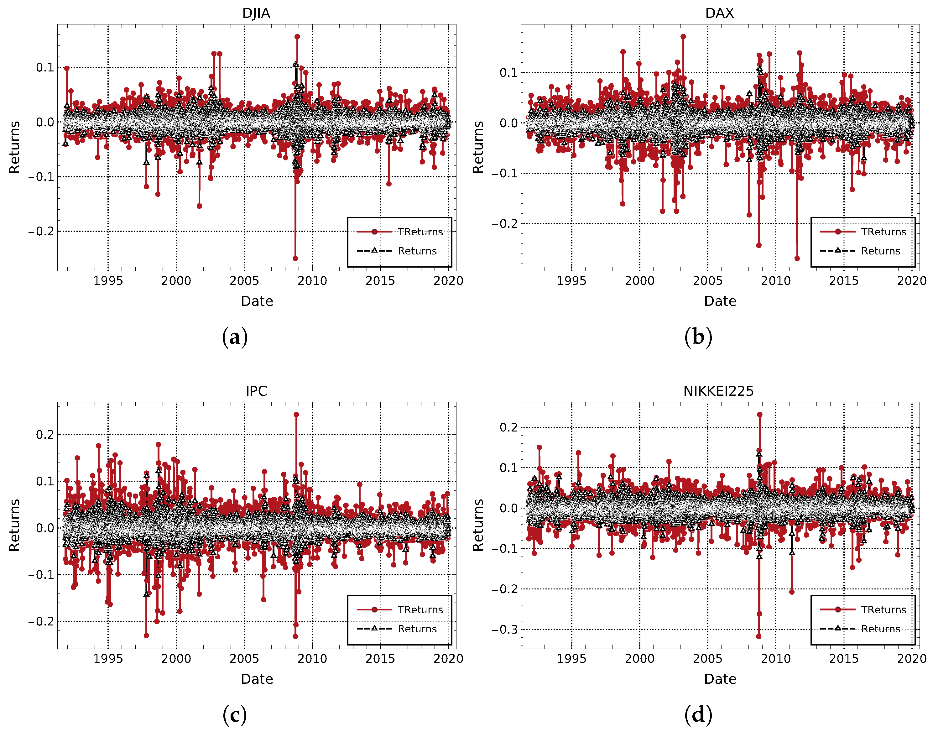
In Figure 2, we can observe the normalized distributions of TReturns for the different markets studied in this paper, whereas Figure 3 displays the corresponding evolution of TReturns over time. It can be appreciated that TReturns mean value in same way as for usual daily returns, fluctuate around zero in addition, no trends are present or may be detected at a glance.

4.1.2. Discussion on TReturns stationarity

Before proceeding further, it is important to establish whether the observable TReturns can be treated as a stationary random variable or not. Returning to Section 4.1.1, Figure 2 and Figure 3 show respectively the distribution of the different markets’ TReturns, and their evolution over time. We can see that TReturns are very similar to usual daily-log returns. Although due their construction, TReturns variations are bigger than those of usual daily returns and alternate their sign consecutively, as explained above in Section 4.1.1. The later property entails important consequences related to the stationarity of TReturns distribution. Once the sign of one term of TReturns time series is known, we can know the sign of every other term; this should be reflected in long range correlations displayed by TReturns’ auto correlation function (ACF). At first sight, the later fact seems to be a problem, because ACF of time series generated by stationary random processes have no memory and must decay to zero fast. Even some statistical tests of stationarity are based in the ACF and statistical independence of a time series, as for example the Ljung-Box test [57]. Thereby, TReturns distribution can not be strictly stationary, in fact neither usual daily log-returns are strictly stationary, because the returns’ second central moment it is not constant. Since, (1) returns mean value is constant; (2) returns variance is finite and (3) returns ACF is negligible with the exception of small intraday time scales and then corresponding autocovariance decays promptly to zero (making the autocovariance C o v ( X t , X t + h ) dependent only on h for all index value t, the original third necessary condition required for wide sense stationarity of a stochastic process X t ), it is said that returns are stationary in the weak or wide sense, which is a less restrictive definition of stationarity [58,59].
For the case of TReturns, and although conditions (1) and (2) are fulfilled, condition (3) is not. Consequently, the TReturns variable is not weak stationary. It is interesting that TReturns alternating sign property triggers also an alternating sign behavior of ACF that causes the ACF mean value to decay fast and stay close to zero. Property that deserves a further and deeper study along with its implications on stationarity of TReturns. For example, and due to the aforementioned, TReturns distribution would not pass a stationarity test based in ACF properties, as the mentioned Ljung-Box test, however TReturns distribution may pass other stationarity tests as shown below for the case of the Dickey-Fuller test [60].
Nevertheless, remember that there are other degrees and definitions of a stationary process, which are still less restrictive than weak stationarity. Following [59], TReturns are compatible with the definition of stationarity up to order m = 1 or first order stationary, i.e., TReturns first central moment is constant. Again, since its second central moment depends on volatility and then cannot be constant, TReturns variable is not stationary up to order m = 2 .
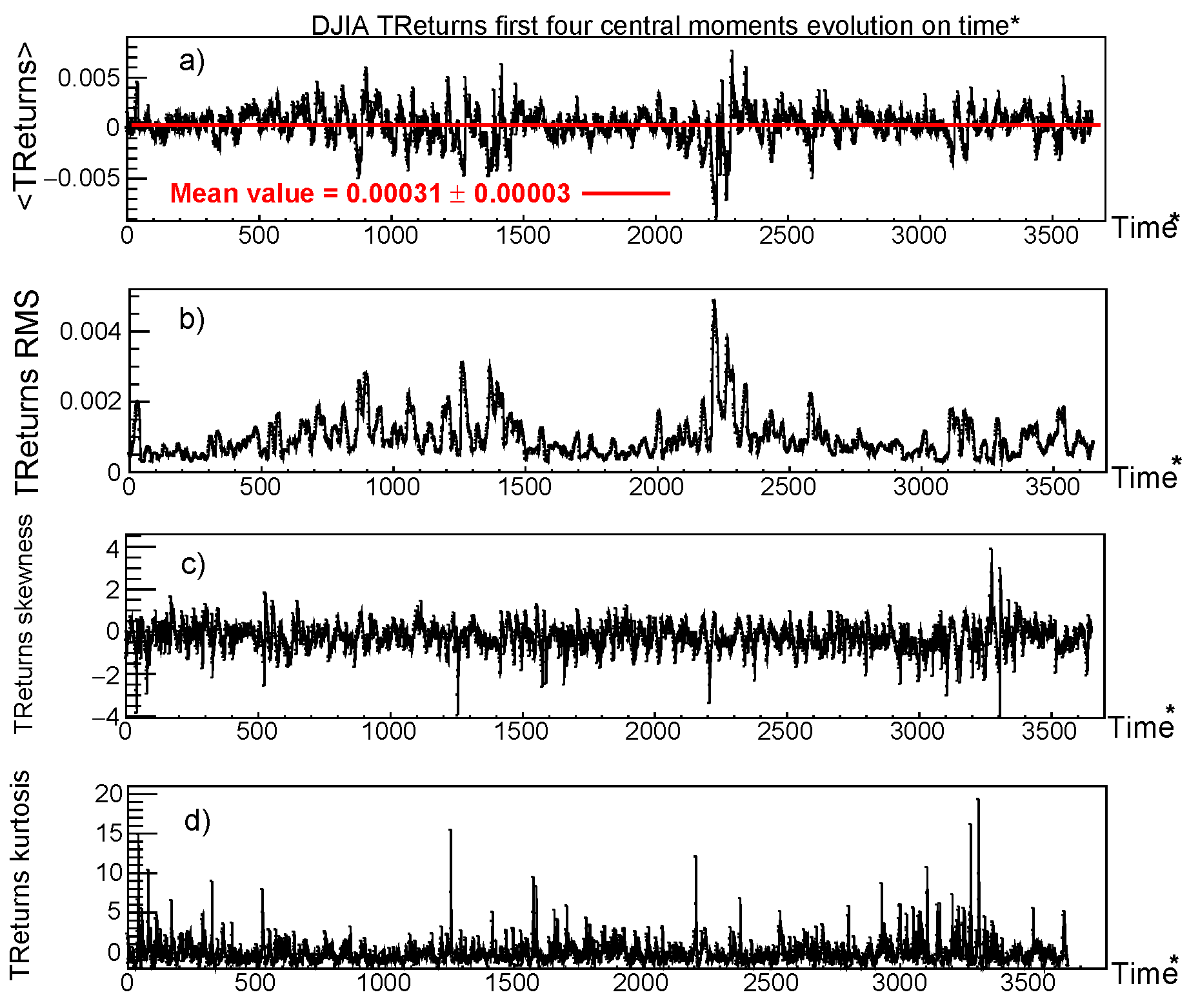
Indeed, it is reasonable to accept that TReturns first central moment is constant. To motivate this, for DJIA, in Figure 4, by using a moving average with a time window of 25 days, we show the behavior on time of the first four central moments of TReturns distribution. At a glance, no trends are detected in the evolution of T R e t u r n s . RMS at Figure 4 must be a multi-scale volatility measurement that deserves additional study, and can not be constant. Skewness could be handled as constant and kurtosis seems at least stationary. First moment T R e t u r n s evolution does not show trends and fluctuates around its mean value, signaled in Figure 4 by a straight, horizontal red line, with a value of 0.00031   ±   0.00003 .
Unlike plots from Figure 3 where TReturns duration was scaled to “real” (chronological) time, in Figure 4, we denote the independent, horizontal variable by T i m e * to indicate that every time unit in the horizontal axis corresponds to the trend duration of the corresponding displayed TReturn, which may last from one to several days.
The Dickey-Fuller test is a type of unit root test that performs a hypothesis test on a time series with the null hypothesis that a unit root is present in an autoregressive time series model. Having a result of a small p-value suggests that the presence of a unit root is unlikely. By rejecting the null hypothesis, it allows the conclusion that the sample data could have come from a stationary time series. We perform a Dickey-Fuller test on two time series of Returns and TReturns constructed from prices of the DJIA partitioned in sets of 25 days. By setting a significance level of 0.05, results show that for both Returns and TReturns, the time series behaves as a mostly stationary process, with the exception of three single events on the Returns where non-stationarity cannot be discarded. This is shown in Figure 5.
From the above discussion, in our opinion, it is possible to statistically treat TReturns in same way as we treat usual daily log-returns.

4.1.3. Trader’s Operation Rules

Again, before explaining the rules that determine how traders operate, we must remind that the traders described here are not agents in the sense of simulation of agents’ methodologies (agent based simulations). They do not interact between themselves exchanging information or money or something else. The optimal trader buys and sells the index, exactly in the best moment to maximize returns, which of course is something impossible in practice; on the other hand, the noise traders alternate long and short positions, keeping them a random number of days, as will be explained below. No transaction fees are considered. So, our traders are more competing algorithms processing real data than interacting agents.
Given a financial time series of prices or financial index values, we are interested in the sub-series or sub-sequence of s successive trend durations k 1 , k 2 , k 3 , , k s observed in real data. Traders operate as follows:
Definition 7
(Operational definition of the optimal trader). The optimal trader is that one that opens a long position at the beginning of an uninterrupted uptrend and closes it at the end of it, i.e., at the extreme and maximum value of this trend to immediately proceed to open a short position at the beginning of the uninterrupted downtrend and closing this short position at the lowest value of the downtrend, i.e., the extreme and minimum value of this downtrend, then the trader repeats this procedure until the end of the given financial time series. No transaction fees are considered.
Following this trading rule, the returns of the optimal trader will be:
| T R m 1 k 1 ( ϵ 1 ) | , | T R m 2 k 2 ( ϵ 2 ) | , | T R m 3 k 3 ( ϵ 3 ) | , , | T R m s k s ( ϵ s ) |
All these TReturns are positive because the optimal trader goes long during uptrends and goes short during downtrends. Optimal trader total returns, denoted T o t R e t s , is only the sum of the overall of the returns (6) as follows:
T o t R e t s ; = i = 1 s | T R m i k i ( ϵ i ) |
Clearly, the list of durations of observed uninterrupted trends { k 1 , k 2 , , k s } are the time scales corresponding to every calculated TReturn.
On the other hand, noise traders open, hold and close, alternating long and short positions as follows:
Definition 8.
Operational definition of a noise trader: For every j t h noise trader, j = 1 , 2 , , N N T = 1000 , a corresponding random sequence D j of integers, representing random trend durations, is generated, where
D j = { d j 1 , d j 2 , , d j s }
is such that d j 1 + d j 2 + + d j s = n , where s and n are correspondingly, the number of uninterrupted trends and the number of entries of the particular financial index studied and displayed at last column of Table 1.
Then, the j t h noise trader alternately opens and closes long and short positions on the real financial index data without any fee cost, accordingly with the records of the random sequence D j .
The integers belonging to the sequence D j = { d j 1 , d j 2 , , d j s } , are generated following an uniform random distribution in the interval [ 1 , m m a x ] , where m m a x = M a x i m u m { k 1 , k 2 , , k s } , is the duration in days of the longest trend observed in real data.
Here, we must say that for this study, we have chosen the simplest way of generating returns for the noise traders using the selected financial data samples. We could have generated the synthetic trends durations for the random traders using random numbers following an exponential distribution, a more realistic option [61], or by sorting the { k 1 . k 2 , , k s } observed trend durations, to have s ! sequences of integers to generate noise traders returns. This approach will be explored in a future paper.

5. Results of the Data Analysis

The overall returns distribution of 1000 noise traders and TReturn distributions of the optimal trader, for the four studied markets, are displayed in Figure 6. We must remember that since the optimal trader never leaves a coin on the table, and it does not experience any loss, its returns are always positive.
Table 2 displays the statistical descriptive values of returns distributions shown in Figure 6.
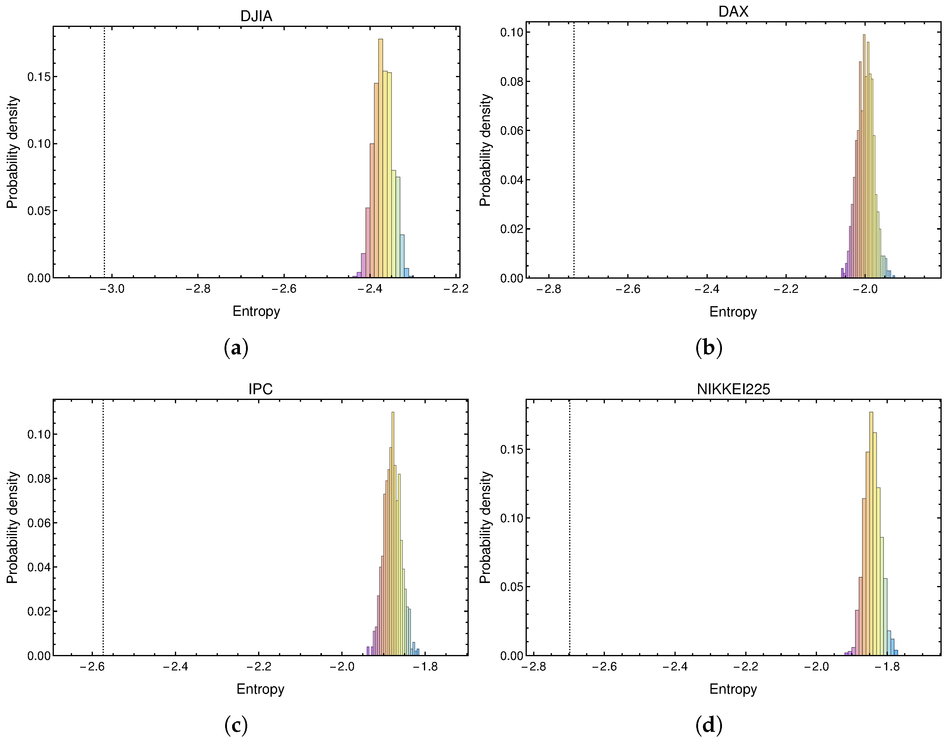
Entropy distribution of returns of noise traders and the value of entropy of the optimal trader returns, for each one of the analyzed markets can be observed in the four panels of Figure 7. Since there is a non null probability for any noise trader of inputting a data time sub-series as shown in Equation (8) with durations identical to the observed in real data, is clear that the optimal trader’s entropy value signaled with a pointed line in each one of these plots in Figure 7, is a noteworthy and legitimate outlier of entropy distribution for returns of all traders. More on this issue will be discussed at the end of the current subsection.
Descriptive statistics of the entropy of noise traders returns distributions for all analyzed markets are displayed in Table 3.
Table 4 displays the values of entropy for the optimal traders returns distribution signaled as dotted lines in Figure 7 for all analyzed markets, as well as how many standard deviations are far away from the mean value of entropy distributions of noise traders returns.
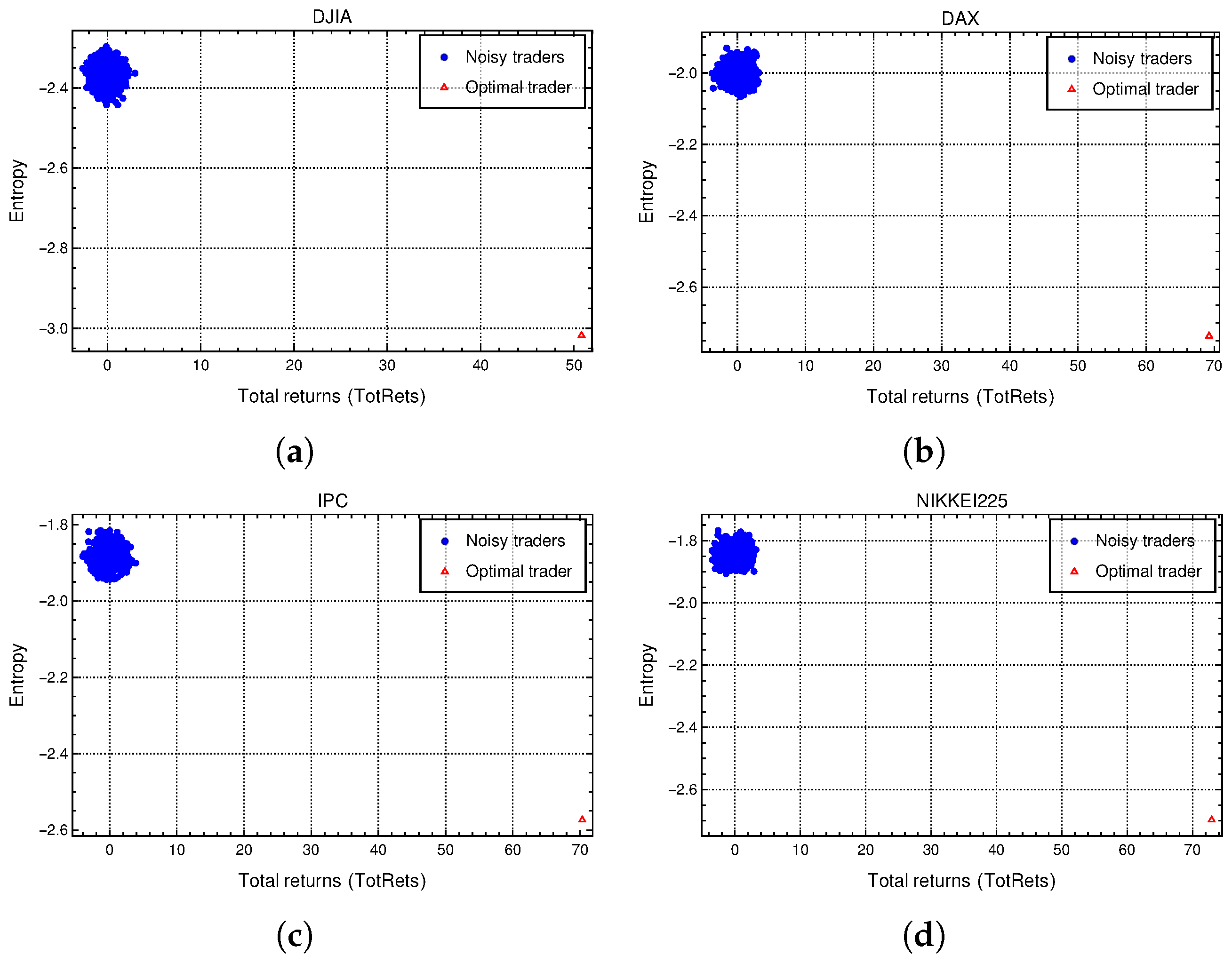
Of course, we would also expect that total returns as defined by Equation (7) of the optimal traders to be outliers of noise traders Total Returns distribution. Figure 8 shows the scatter plot of entropy vs. Total Returns for all traders and confirms this fact. In this figure, small red triangles mark the point (total return, entropy) corresponding to the optimal traders of the four markets studied.
Do not forget that, since returns of optimal traders are logarithmic, they are adimensional, so they are not given in monetary units.

5.1. Kullback-Leibler Divergence Analysis

To finish our entropy analysis, we show in Figure 9 the distribution of Kullback-Leibler (KL) divergence between each one of the noise traders and the corresponding optimal trader for each studied market. Descriptive statistics of these distributions is displayed in Table 5.
From Equation (3) it is clear that for any two probability density functions p ( x ) and q ( x ) , that D K L ( p ( x ) | | q ( x ) ) D K L ( q ( x ) | | p ( x ) ) , i.e., Kullback Leibler divergence depends of the order in which p ( x ) and q ( x ) are taken. Having this fact in mind and in order to have an idea of the distance between returns distributions of the four optimal traders, we display in Table 6, the KL Divergence tabulated of all possible pairs of them:
As will be argued in Section 5.2, it is well known that the most mature and efficient of the studied markets is the DJIA. Using this fact, we will take as reference the value of KL divergence between DJIA TReturns of the optimal trader and all other markets. Table 6 of KL divergence values between the TReturns distributions of the different optimal traders and the DJIA optimal trader allow us to order the different markets listed according to KL divergence values relative to DJIA TReturns, from lower to higher divergence as DJIA, DAX, Nikkei and IPC. As can be observed in Table 6, these results did not depend of the order of the pairs taken to calculate KL divergence. We will discuss these results on the order obtained by calculating KL divergences between the different studied markets in the context of markets efficiency in Section 5.2 and in Section 6 (Conclusions).

5.2. A Simple Application: Ranking the Studied Markets by Their OT Entropy

Shannon’s entropy has been used to quantify average uncertainty, information or complexity of a random variable or outcomes of an experiment expressed as a time series. In the context of our study, we construct multi-scale returns of the optimal traders, and we know that they act as having full market information to trade accordingly to obtain the maximum returns possible, and then we analyze their entropy. In this sense, the entropy measures obtained for the different markets may be related with market efficiency.
To have a bigger picture of our entropy measurements of an optimal trader returns, the measurement of the entropy of optimal traders returns distributions, entry by entry are plotted in Figure 10. Here, the value of the entropy of the optimal trader returns at the end of every uninterrupted trend is plotted. We call this measurement accumulative entropy for a trader, because for a time series of multi-scale returns for a particular trader, its value at time t i is obtained by calculating the entropy of the overall of the i first entries of the time series of multi-scale returns and then plotting the corresponding point. Following this procedure for all entries, at the end, we obtain the respective entropy values of Table 4 that corresponds to the entropy of the overall of the optimal traders returns distribution for the four markets analyzed here.
From Figure 10 and minimal values of entropy shown in Figure 7, it is roughly concluded that the markets studied in this paper can be ordered from higher to lower entropy values as follows: (1) DJIA, (2) DAX, (3) Nikkei and (4) IPC. Another assertion we can make is that, since Figure 10 shows that entropy is decreasing over time for all studied markets. On the other hand, we also know that a general increase of efficiency over time is observed in worldwide financial markets as has been reported in different empirical studies of financial indices and prices time series [62,63]. This later fact also agrees with the higher efficiency observed in more mature and well established financial markets as, for example, the DJIA in comparison with emergent markets [64,65,66].
In the previous paragraph, we use the word “roughly”, because given the way we calculate and plotted this “accumulative entropy”, it is not possible to observe more detailed entropy fluctuations. This is expected because the addition of only one next, singular value of a trader’s returns does not change significantly the corresponding entropy value, especially after a great number of time steps.
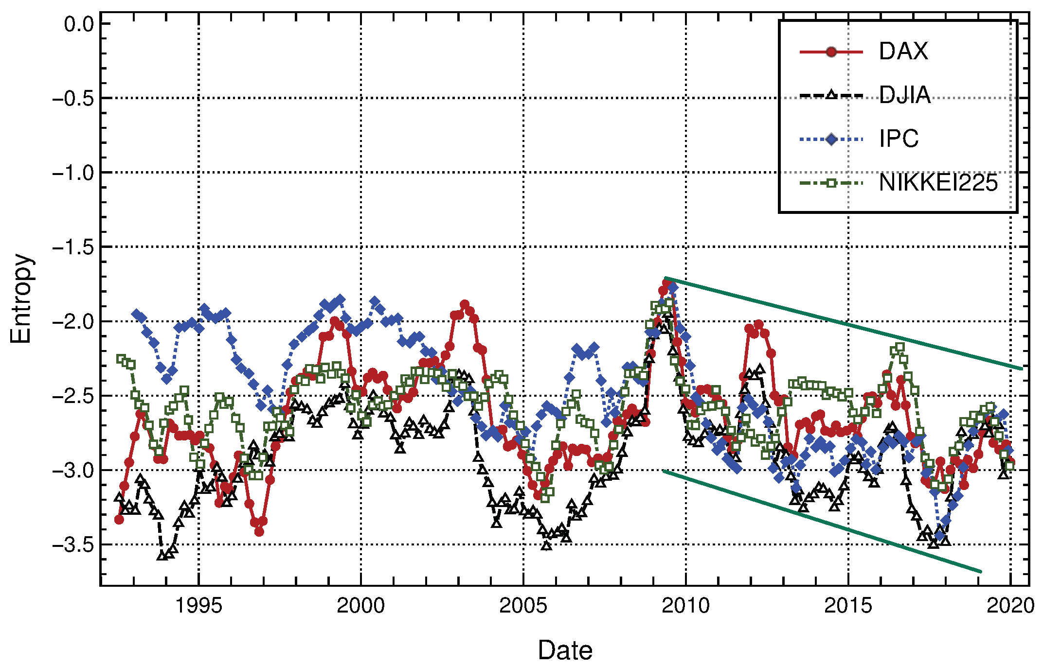
To complement this study and in order to be able to observe more detailed entropy fluctuations, in Figure 11 we again show the time evolution of entropy for the four optimal traders returns, this time using a time window of 100 uninterrupted trend durations. We sharpen our previous conclusions: (1) DJIA and IPC markets maintain their entropy rank pointed out above, with DJIA being the first ranked market, IPC the last ranked and Nikkei and DAX exchanging second and third positions over time. Some spans where these positions change are observed, for example Nikkei ranked last from 2013 to 2017; (2) All studied markets decrease their entropy as time goes on, in fact for all markets, since a noteworthy 2009 entropy peak, a downtrend in entropy values is observed in Figure 10 and remarked by parallel trend lines. It is possible appreciate four entropy peaks, with every next one being lower than the previous one, where the same can be said for all entropy minimum values observed since then. Even more, during the second half of the year 2018 up to 2020, entropy fluctuations for all markets are very similar.
To end this section, we cannot fail to notice that markets rank presented here, obtained by the entropy criterion, seems to coincide with the one we would obtain by ranking the studied markets by their respective efficiency.

6. Conclusions

We have presented an empirical data analysis of entropy of returns distribution for two kind of traders:
  • An optimal trader that represents an ideally rational, fully informed and then a perfect forecaster, a market participant which obtains a maximum return in every trade, opening alternately long and short positions exactly when real data daily uninterrupted uptrends and downtreds, start and end, respectively, and closing alternately these positions exactly at the right time to obtain optimum returns, i.e., selling long positions at the end of the uninterrupted uptrend and buying them back when the corresponding uninterrupted downtrend finishes.
  • One thousand noise traders, which trade opening and closing alternately long and short positions during uniformly distributed random spans of days over real data, with the only restriction being that the overall addition of the duration of these time spans is equal to the total number of days of the corresponding financial time series analyzed.
Therefore, in order to generate respective returns distribution, every noise trader inputs a uniformly distributed random generated sequence of integers, representing uninterrupted trend durations. The probability of a trader of being fed with exactly the same sequence of uninterrupted trend duration observed in real data for an optimal trader is truly very low, but non null. In this sense, the records of the entropy of the four optimal traders shown in Figure 7 are valid outliers of their respective entropy distribution of all traders.
Returns of the optimal trader involve non-arbitrary different time scales, making this observation worthy of further study [45].
Entropy is calculated from the distribution of returns of each trader. We have shown in Figure 7 that, for all markets studied, the entropy of returns distribution of an optimal trader has the lowest value compared with all entropies of noise traders return distributions. These entropy values of optimal traders for all markets are recorded in Table 4. The huge distance in σ units from optimal trader entropy value to the mean entropy value of noise traders are also displayed for all markets in the third column of this table. Obtained returns and entropies values for these two kinds of traders are in agreement with the usual interpretation of entropy as a measure of uncertainty of a random process. Additional studies to see if these measurements are useful to characterize some other market properties still have to be performed, for example studying normalized TReturns involving different markets.
In addition, we ordered each one of the markets studied here by means of the entropy value of its corresponding optimal trader returns distribution. Following this criterion, from higher to lower, the markets can be ranked as: (1) DJIA, (2) DAX, (3) Nikkei and (4) IPC, as is shown in Table 4. This is in agreement with the rank obtained by the values of KL divergence of returns of each optimal trader to the optimal trader returns of the DJIA, the most well known efficient markets of the studied in this work and given in Table 6.
As we mentioned in Section 5.2, we can’t help but notice that ranking of markets obtained by our entropy criterion match the rank of efficiency for the different markets studied here, and reported elsewhere. This is so because given the informational aspect of the EMH and the way we a priori construct a trader with perfect information on the market, which generates maximum returns from whose distribution entropy is calculated; we think that our methodology also can be used to study and rank different markets efficiency. However, a more formal and complete study has still to be performed to provide sufficient evidence supporting the last statement, and this is left for future work.
With respect to our choosing of a uniform distribution to determine noise traders, trade timing it is not arbitrary, we have set up our methodology in the simplest possible way and with the maximum uncertainty, human participants in a “bucket shop” establishment really did not act fully randomly [67] and of course we do not intend in this paper to use or reproduce the pseudo-random number generator “attached” to the human brain, by the other hand, and under the point of view of trends duration just mentioned above, it should be possible to be more realistic and consider that the sequence of generated synthetic periods of time for each noise trader, decays as a geometric or as an exponential distribution [61], with the same exponent that real data uninterrupted trend durations or even by making use of different permutations of the sequence of time durations of uninterrupted trends used to calculate the random variable TReturns could be utilized to calculate returns of noise traders with the advantage of having the option of calculating returns distributions as far or as close in probability as desired to the optimal trader returns distribution. These alternatives should decrease the entropy gap between entropies of noise and the optimal trader returns making noise traders’ returns more realistic. Different measures of complexity may also be explored for comparison with the entropy used in this paper.
Finally, for reasons of completeness, in this work we have presented a discussion and a simple empirical analysis on stationarity of TReturns distribution to show that it makes sense to study TReturns and treat them statistically the same way as usual daily log-returns. In a future work, TReturns statistical properties and particularly stationarity will be studied deeper, as well as other topics just mentioned in the previous paragraphs.

Author Contributions

Conceptualization A.R.H.-M.; methodology, A.R.H.-M.; software, C.M.R.-M., D.H.-E. and M.E.R.-A.; validation, all authors; formal analysis, all authors; investigation, all authors; writing–original draft preparation, A.R.H.-M.; writing–review and editing, all authors; project administration, A.R.H.-M. and M.E.R.-A.; funding acquisition, A.R.H.-M. All authors have read and agreed to the published version of the manuscript.

Funding

This research was funded by Mexican National Council of Science and Technology, Conacyt, under grants numbers 5150 supported by FOINS and grant number 693908.

Institutional Review Board Statement

Not applicable.

Informed Consent Statement

Not applicable.

Data Availability Statement

Mathematica code and data used in the analysis presented in this paper, can be download any time from https://github.com/CarlosManuelRodr/EntropyMarketAnalysis.

Acknowledgments

We have appreciated very much the pertinent suggestions of Thomas H. Seligman. We also thank Selene Jiménez for assistance and Latex revision. Finally, we thank comments and suggestions from anonymous referees, who have improved the rigor and academic level of our manuscript.

Conflicts of Interest

The authors declare no conflict of interest.

References

  1. Mantegna, R.N.; Stanley, H.E. An Introduction to Econophysics: Correlations and Complexity in Finance; Cambridge University Press: Cambridge, MA, USA, 1999. [Google Scholar]
  2. McCauley, J.L. Dynamics of Markets: Econophysics and Finance; Cambridge University Press: Cambridge, MA, USA, 2004. [Google Scholar]
  3. Slanina, F. Essentials of Econophysics Modelling; OUP Catalogue, Oxford University Press: Oxford, UK, 2013. [Google Scholar] [CrossRef] [Green Version]
  4. Richmond, P.; Mimkes, J.; Hutzler, S. Econophysics and Physical Economics; Oxford University Press: Oxford, UK, 2013. [Google Scholar] [CrossRef]
  5. Anderson, P.W. More Is Different. Science 1972, 177, 393–396. [Google Scholar] [CrossRef] [Green Version]
  6. Simon, H.A. The Architecture of Complexity. Proc. Am. Philos. Soc. 1962, 106, 467–482. [Google Scholar]
  7. May, R. Simple mathematical models with very complicated dynamics. Nature 1976, 261, 459–467. [Google Scholar] [CrossRef]
  8. Kwapień, J.; Drożdż, S. Physical approach to complex systems. Phys. Rep. 2012, 515, 115–226. [Google Scholar] [CrossRef]
  9. Haken, H. Synergetics: An Introduction: Nonequilibrium Phase Transitions and Self-Organizatio in Physics, Chemistry and Biology; Springer Series in Synergetics; Springer: Berlin/Heidelberg, Germany, 1978. [Google Scholar]
  10. Tacchella, A.; Cristelli, M.; Caldarelli, G.; Gabrielli, A.; Pietronero, L. A New Metrics for Countries’ Fitness and Products’ Complexity. Sci. Rep. 2012, 2, 723. [Google Scholar] [CrossRef] [Green Version]
  11. Hidalgo, C.A.; Klinger, B.; Barabási, A.L.; Hausmann, R. The Product Space Conditions the Development of Nations. Science 2007, 317, 482–487. [Google Scholar] [CrossRef] [Green Version]
  12. Hausmann, R.; Hidalgo, C.A.; Bustos, S.; Coscia, M.; Simoes, A.; Yıldırım, M.A. The Atlas of Economic Complexity: Mapping Paths to Prosperity; The MIT Press: Cambridge, MA, USA, 2013. [Google Scholar]
  13. Mirowski, P. More Heat Than Light: Economics as Social Physics, Physics as Nature’s Economics; Cambridge University Press: Cambridge, MA, USA; New York, NY, USA,, 1989; 450p. [Google Scholar]
  14. Mimkes, J. Binary alloys as a model for the multicultural society. J. Therm. Anal. 1995, 43, 521–537. [Google Scholar] [CrossRef]
  15. Foley, D. A Statistical Equilibrium Theory of Markets. J. Econ. Theory 1994, 62, 321–345. [Google Scholar] [CrossRef]
  16. Mimkes, J. A Thermodynamic Formulation of Economics. In Econophysics and Sociophysics; John Wiley & Sons, Ltd.: Hoboken, NJ, USA, 2006; Chapter 1; pp. 1–33. [Google Scholar] [CrossRef] [Green Version]
  17. Georgescu-Roegen, N. The Entropy Law and the Economic Process; Harvard University Press: Cambridge, MA, USA, 1971. [Google Scholar]
  18. Chen, J. The Physical Foundation of Economics: An Analytical Thermodynamic Theory; Number 5819 in World Scientific Books; World Scientific Publishing Co. Pte. Ltd.: Singapore, 2005. [Google Scholar]
  19. Li, S.; Zhuang, Y.; He, J. Stock market stability: Diffusion entropy analysis. Phys. A Stat. Mech. Appl. 2016, 450, 462–465. [Google Scholar] [CrossRef]
  20. Uddin, G.S.; Bekiros, S.; Ahmed, A. The nexus between geopolitical uncertainty and crude oil markets: An entropy-based wavelet analysis. Phys. A Stat. Mech. Appl. 2018, 495, 30–39. [Google Scholar] [CrossRef]
  21. Gu, R. Multiscale Shannon entropy and its application in the stock market. Phys. A Stat. Mech. Appl. 2017, 484, 215–224. [Google Scholar] [CrossRef]
  22. Ormos, M.; Zibriczky, D. Entropy-Based Financial Asset Pricing. PLoS ONE 2015, 9, e115742. [Google Scholar] [CrossRef] [PubMed]
  23. Jakimowicz, A. The Role of Entropy in the Development of Economics. Entropy 2020, 22, 452. [Google Scholar] [CrossRef]
  24. Ruch, E. The diagram lattice as structural principle A. New aspects for representations and group algebra of the symmetric group B. Definition of classification character, mixing character, statistical order, statistical disorder; A general principle for the time evolution of irreversible processes. Theor. Chim. Acta 1975, 38, 167–183. [Google Scholar] [CrossRef]
  25. Ruch, E.; Schranner, R.; Seligman, T.H. Generalization of a Theorem by Hardy, Littlewood and Polya. J. Math. Anal. Appl. 1980, 76, 222–229. [Google Scholar] [CrossRef] [Green Version]
  26. Swendsen, R.H. Thermodynamics, Statistical Mechanics and Entropy. Entropy 2017, 19, 603. [Google Scholar] [CrossRef] [Green Version]
  27. Buonsante, P.; Franzosi, R.; Smerzi, A. On the dispute between Boltzmann and Gibbs entropy. Ann. Phys. 2016, 375, 414–434. [Google Scholar] [CrossRef] [Green Version]
  28. Županović, P.; Kuić, D. Relation between Boltzmann and Gibbs entropy and example with multinomial distribution. J. Phys. Commun. 2018, 2, 045002. [Google Scholar] [CrossRef]
  29. Liu, A.; Chen, J.; Yang, S.; Hawkes, A. The Flow of Information in Trading: An Entropy Approach to Market Regimes. Entropy 2020, 22, 1064. [Google Scholar] [CrossRef]
  30. Chakraborti, A.; Hrishidev, K.; Hirdesh, K. Phase separation and scaling in correlation structures of financial markets. J. Phys. Complex. 2021, 2, 015002. [Google Scholar] [CrossRef]
  31. Steeg, V.; Galstyan, A. Information transfer in social media. In Proceedings of the 21st International Conference on World Wide Web, Lyon, France, 16–20 April 2012; pp. 509–518. [Google Scholar]
  32. Sandoval, L. Structure of a Global Network of Financial Companies Based on Transfer Entropy. Entropy 2014, 16, 4443–4482. [Google Scholar] [CrossRef] [Green Version]
  33. Bekiros, S.; Nguyen, D.; Sandoval, L.; Uddin, G. Information Diffusion, Cluster formation and Entropy-based Network Dynamics in Equity and Commodity Markets. Eur. J. Oper. Res. 2017, 256, 945–961. [Google Scholar] [CrossRef] [Green Version]
  34. Barnett, L.; Barrett, A.; Seth, A. Granger causality and transfer entropy are equivalent for Gaussian variables. Phys. Rev. Lett. 2009, 103, 238701. [Google Scholar] [CrossRef] [PubMed] [Green Version]
  35. Amblard, P.; Michel, O. The relation between Granger causality and directed information theory: A review. Entropy 2013, 15, 113–143. [Google Scholar] [CrossRef] [Green Version]
  36. Liu, L.; Hu, H.; Deng, Y.; Ding, N. An entropy measure of non-stationary processes. Entropy 2014, 16, 1493–1500. [Google Scholar] [CrossRef]
  37. Nichols, J.; Bucholtz, F.; Michalowicz, J. Linearized transfer entropy for continuous second order systems. Entropy 2013, 15, 3186–3204. [Google Scholar] [CrossRef]
  38. Prokopenko, M.; Lizier, J.; Price, D. On thermodynamic interpretation of transfer entropy. Entropy 2013, 15, 524–543. [Google Scholar] [CrossRef] [Green Version]
  39. Dimpfl, T.; Peter, F. Using transfer entropy to measure information flows between financial markets. Stud. Nonlinear Dyn. Econom. 2013, 17, 85–102. [Google Scholar] [CrossRef] [Green Version]
  40. Kukreti, V.; Hirdesh, K.; Gupta, P.; Kumar, S. A Perspective on Correlation-Based Financial Networks and Entropy Measures. Front. Phys. 2020, 8, 323. [Google Scholar] [CrossRef]
  41. Lefevre, E. Reminiscences of a Stock Operator; Wiley Investment Classics, John Wiley and Sons, Inc.: Hoboken, NJ, USA, 2006. [Google Scholar] [CrossRef]
  42. Hochfelder, D. Where the Common People Could Speculate: The Ticker, Bucket Shops, and the Origins of Popular Participation in Financial Markets, 1880–1920. J. Am. Hist. 2006, 93, 335–358. [Google Scholar] [CrossRef]
  43. Morris, J. Bucket Shops. Am. Political Sci. Rev. 1907, 2, 48–50. [Google Scholar] [CrossRef]
  44. Bricklin, J. King of the Bucket Shops. Financ. Hist. 2013, 105, 23–25. [Google Scholar]
  45. Martínez-Rodríguez, C.M.; Coronel-Brizio, H.F.; Hernández-Montoya, A.R. A multi-scale symmetry analysis of uninterrupted trends returns of daily financial indices. Physica A 2021, 574, 125982. [Google Scholar] [CrossRef]
  46. Shannon, C.E. A Mathematical Theory of Communication. Bell Syst. Tech. J. 1948, 27, 623–656. [Google Scholar] [CrossRef]
  47. Tsallis, C. Possible generalization of Boltzmann-Gibbs statistics. J. Stat. Phys. 1988, 52, 479–487. [Google Scholar] [CrossRef]
  48. Rényi, A. On Measures of Entropy and Information. In Proceedings of the Fourth Berkeley Symposium on Mathematical Statistics and Probability; Volume 1: Contributions to the Theory of Statistics; University of California Press: Berkeley, CA, USA, 1961; pp. 547–561. [Google Scholar]
  49. Fama, E.F. Efficient Capital Markets: A Review of Theory and Empirical Work. J. Financ. 1970, 25, 383–417. [Google Scholar] [CrossRef]
  50. Daigler, R.T.; Wiley, M.K. The Impact of Trader Type on the Futures Volatility-Volume Relation. J. Financ. 1999, 54, 2297–2316. [Google Scholar] [CrossRef]
  51. Bloomfield, R.; O’Hara, M.; Saar, G. How Noise Trading Affects Markets: An Experimental Analysis. Rev. Financ. Stud. 2009, 22, 2275–2302. [Google Scholar] [CrossRef]
  52. Malkiel, B.G. The Efficient Market Hypothesis and Its Critics. J. Econ. Perspect. 2003, 17, 59–82. [Google Scholar] [CrossRef] [Green Version]
  53. Keane, S. The Efficient Market Hypothesis on Trial. Financ. Anal. J. 1986, 42, 58–63. [Google Scholar] [CrossRef]
  54. Engel, C.; Morris, C.S. Challenges to stock market efficiency: Evidence from mean reversion studies. Econ. Rev. 1991, 76, 21–35. [Google Scholar]
  55. Ying, Q.; Yousaf, T.; Ain, Q.U.; Akhtar, Y.; Rasheed, M.S. Stock Investment and Excess Returns: A Critical Review in the Light of the Efficient Market Hypothesis. J. Risk Financ. Manag. 2019, 12, 97. [Google Scholar] [CrossRef] [Green Version]
  56. Le Tran, V.; Leirvik, T. A simple but powerful measure of Market Efficiency. Financ. Res. Lett. 2019, 29, 141–151. [Google Scholar] [CrossRef]
  57. Box, G.E.P.; Pierce, D.A. Distribution of Residual Autocorrelations in Autoregressive-Integrated Moving Average Time Series Models. J. Am. Stat. Assoc. 1970, 65, 1509–1526. [Google Scholar] [CrossRef]
  58. Anderson, T.W. The Statistical Analysis of Time Series; Wiley: Hoboken, NJ, USA, 1971. [Google Scholar]
  59. Priestley, M.B. Spectral Analysis and Time Series; Academic Press: Cambridge, MA, USA, 1981; Volume 1. [Google Scholar]
  60. Dickey, D.A.; Fuller, W.A. Distribution of the Estimators for Autoregressive Time Series With a Unit Root. J. Am. Stat. Assoc. 1979, 74, 427–431. [Google Scholar] [CrossRef]
  61. Li, H.; Gao, Y. Statistical distribution and time correlation of stock returns runs. Physica A 2007, 377, 193–198. [Google Scholar] [CrossRef]
  62. Tótha, B.; Kertész, J. Increasing market efficiency: Evolution of cross-correlations of stock returns. Physica A 2005, 360, 505–515. [Google Scholar] [CrossRef] [Green Version]
  63. Coronel-Brizio, H.F.; Hernández-Montoya, A.R.; Huerta-Quintanilla, R.; Rodríguez-Achach, M.E. Evidence of increment of efficiency of the Mexican Stock Market through the analysis of its variations. Physica A 2007, 380, 391–398. [Google Scholar] [CrossRef] [Green Version]
  64. Eoma, C.; Choi, S.; Oh, G.; Jung, W.S. Hurst exponent and prediction based on weak-form efficient market hypothesis of stock markets. Physica A 2008, 387, 4630–4636. [Google Scholar] [CrossRef] [Green Version]
  65. Zalewska-Mitura, A.; Hall, S.G. Examining the first stages of market performance: A test for evolving market efficiency. Econ. Lett. 1999, 64, 1–12. [Google Scholar] [CrossRef] [Green Version]
  66. Di Matteo, T.; Astea, T.; Dacorogna, M. Scaling behaviors in differently developed markets. Physica A 2003, 324, 183–188. [Google Scholar] [CrossRef]
  67. Schulz, M.; Schmalbach, B.; Brugger, P.; Witt, K. Analysing Humanly Generated Random Number Sequences: A Pattern-Based Approach. PLoS ONE 2012, 7, e41531. [Google Scholar] [CrossRef]
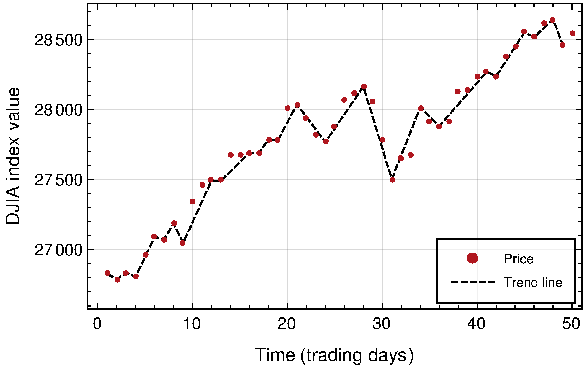
Figure 1. Illustration of uninterrupted uptrends and downtrends definition from a daily DJIA time series from 21 October 2019 to 31 December 2019. The pointed line indicates the alternated uninterrupted downtrends and uptrends.
Mathematics 10 00215 g001
Figure 2. Multi-scale returns distributions (normalized histograms) for all studied markets: (a) in a linear scale, and (b) in a log-vertical scale.
Mathematics 10 00215 g002
Figure 3. TReturns and daily log-returns evolution for all studied markets. (a) DJIA, (b) DAX, (c) IPC and (d) Nikkei data samples.
Mathematics 10 00215 g003
Figure 4. Four first central moments evolution for DJIA. (a) T R e t u r n s vs. T i m e * , overall mean value is signaled by the red, straight line and has a value of 0.00031   ±   0.00003 . (b)TReturns RMS as a function of T i m e * . (c) TReturns skewness evolution on T i m e * . (d) TReturns kurtosis evolution on T i m e * . Figures were plotted by using a 25 days Moving Average on DJIA TReturns time series.
Mathematics 10 00215 g004
Figure 5. Stationarity Dickey-Fuller test applied to DJIA daily log-returns and TReturns time series using a time window of 25 days. Pointed line signals the α = 0.05 significance level. Both time series passed the test, with the only exception of three single events for TReturns visible in the plot.
Mathematics 10 00215 g005
Figure 6. Returns distributions (normalized histograms) for all studied markets of the optimal trader (continuous blue line) and the 1000 noise traders (pointed red line) for: (a) DJIA, (b) DAX, (c) IPC and (d) Nikkei data samples. By its definition, the optimal trader does not have negative returns.
Mathematics 10 00215 g006
Figure 7. Entropy distributions (normalized histograms) of returns for the overall of traders for each studied market corresponding to: (a) DJIA, (b) DAX, (c) IPC and (d) Nikkei indices. Value of entropy corresponding to the optimal trader returns for each one of these markets is signaled with a vertical dotted line and is smaller than any noise trader’s returns entropy value. Note that because we used differential entropy definition for a continuous variable, entropy values can be negative.
Mathematics 10 00215 g007
Figure 8. Scatter plot of entropy vs. total returns, or TotRets for all traders. Red triangles in the right lower corners, indicate the optimal trader values of TotRets and entropy for all markets. TotRets are defined in Equation (7): (a) DJIA, (b) DAX, (c) IPC and (d) Nikkei data samples.
Mathematics 10 00215 g008
Figure 9. Distributions (normalized histograms) of KL divergence of returns distribution of noise traders to optimal trader returns distribution for all studied markets: (a) DJIA, (b) DAX, (c) IPC and (d) Nikkei data samples.
Mathematics 10 00215 g009
Figure 10. Optimal trader’s accumulative entropy evolution over time for our four data samples. A general decrease of OT entropy for all markets is observed since 2010.
Mathematics 10 00215 g010
Figure 11. Optimal trader’s entropy evolution on time for our four data samples using a time window of 100 trend duration in days, i.e., a time period of about four years. Parallel straight lines indicate a clear decrement trend in entropy for the four studied markets. Clearly, since 2009, consecutive peaks in entropy decrease, as do consecutive minimums.
Mathematics 10 00215 g011
Table 1. Data sample analyzed in this work. Records are used to construct our observables as explained below.
Index MarketPeriodEntries
DJIA11/08/1991 to 31/12/20197126
DAX11/08/1991 to 30/12/20197112
IPC11/08/1991 to 31/12/20197038
Nikkei11/10/1991 to 30/12/20196911
Table 2. Descriptive statistics of noise (NT) and optimal trader’s (OT) returns.
ValuesOTNTOTNTOTNTOTNT
DJIADJIADAXDAXIPCIPCNikkeiNikkei
μ 0.0139−1.3   ×   10 5 0.0192 7.8   ×   10 5 0.0218 −6.1   ×   10 5 0.0203 5.7   ×   10 5
± 0.0003 ±2.4   ×   10 5 ±0.0003±3.5   ×   10 5 ±0.0004±4.0   ×   10 5 ±0.0003±4.5   ×   10 5
σ 0.01560.024640.02130.035290.02520.040170.02120.04028
±0.0002±2   ×   10 5 ±0.0003±2   ×   10 5 ±0.0003±3   ×   10 5 ±0.0002±3   ×   10 5
Skewness3.61180.01363.05840.01562.8481−0.00843.2176−0.0115
±0.0405±0.0023±0.0408±0.0024±0.0431±0.0024±0.0409±0.0027
Kurtosis31.01559.608719.96248.137515.42006.875626.27147.5505
±0.9997±0.9999±0.9997±0.9999±0.9999±0.999999±0.9997±0.9999
Table 3. Descriptive statistics of entropy of noise traders (NT) returns.
Market IndexNT Mean EntropyRMSSkewnessKurtosis
DJIA−2.3686 ± 0.00070.0207 ± 0.0005−0.0874 ± 0.07732.9649 ± 0.9990
DAX−1.9997 ± 0.00070.0219 ± 0.0005−0.0113 ± 0.07732.7297 ± 0.9990
IPC−1.8785 ± 0.00070.0208 ± 0.0005−0.0296 ± 0.07733.0562 ± 0.9990
Nikkei225−1.8404 ± 0.00070.0225 ± 0.00050.0211 ± 0.07732.8870 ± 0.9990
Table 4. Optimal trader (OT) entropy values and their distance to mean value of noise traders returns entropy distribution in RMS units.
Market IndexOT Entropy ValueNumber of σ s from Entropy Mean Value
of Noise Traders Returns
DJIA−3.017631.3527 σ
DAX−2.736433.6393 σ
IPC−2.573733.4231 σ
Nikkei225−2.697838.1067 σ
Table 5. From Figure 9, descriptive statistics of KL divergence distribution between noise traders and the corresponding optimal trader for the four studied markets.
Market Index<KL Distance> σ SkewnessKurtosis
DJIA1.1146 ± 0.00170.0541 ± 0.0012−0.1648 ± 0.07734.8231 ± 0.9990
DAX1.0461 ± 0.00170.0533 ± 0.00120.0472 ± 0.07732.9870 ± 0.9990
IPC0.9920 ± 0.00180.0564 ± 0.00130.1567 ± 0.07732.8845 ± 0.9990
Nikkei2250.9632 ± 0.00170.0546 ± 0.00120.1269 ± 0.07732.7134 ± 0.9990
Table 6. KL divergence between all couples of optimal traders returns distributions.
Market IndexDJIADAXIPCNikkei
DJIA0.00.05230.09100.0841
DAX0.05900.00.01180.0078
IPC0.11520.01310.00.0130
Nikkei2250.09080.00900.01160.0
Publisher’s Note: MDPI stays neutral with regard to jurisdictional claims in published maps and institutional affiliations.