Partial Anti-Synchronization Problem of the 4D Financial Hyper-Chaotic System with Periodically External Disturbance

Abstract

This paper is concerned with the partial anti-synchronization of the 4D financial hyper-chaotic system with periodically external disturbance. Firstly, the existence of the partial anti-synchronization problem for the nominal 4D financial system is proven. Then, a suitable filter is presented, by which the periodically external disturbance is asymptotically estimated. Moreover, two disturbance estimator (DE)-based controllers are designed to realize the partial anti-synchronization problem of such a system. Finally, numerical simulation verifies the effectiveness and correctness of the proposed results.

1. Introduction

Since Pecora and Carroll first presented chaos synchronization [1] in 1990, the synchronization problem of chaotic systems has been widely applied in engineering, science, and communications [2,3,4,5,6]. Many types of synchronization problems have been examined, such as complete synchronization, anti-synchronization, lag synchronization, projective synchronization, and so on. Anti-synchronization [7,8,9,10,11,12,13] is an important type of synchronization. It is a phenomenon whereby the state vectors of the slave systems have the same amplitude but opposite signs to those of the master system, i.e., the sum of two signals is expected to converge to zero when anti-synchronization appears. This type of synchronization has found distinctive applications in some fields, such as in communication systems, in which the system’s security and secrecy can be deeply strengthened by transforming from complete synchronization and anti-synchronization periodically in the process of digital signal transmission. As is shown in [7], the existence of the anti-synchronization problem is $f(-x)=-f\left(x\right)$ for a given chaotic system $\dot{x}=f\left(x\right)$. It should be pointed out that the famous Lorenz system does not meet this necessary condition. A natural question arises as to whether the variables of chaotic systems meet such a condition or not. Recently, the partial anti-synchronization [14] was presented, which is a new kind of synchronization and is introduced in the next section.

Consider the following nonlinear system

$$\dot{x}=f\left(x\right)$$

(1)

where $x\in R^n$ is the state, and $f\left(x\right)\in R^n$ is a continuous function.

There exists a non-singular transformation ${(X,Z)}^T=Px$ by which the system (1) can be divided into the following two subsystems:

$$\dot{X}=M(X,Z)$$

(2)

$$\dot{Z}=G(X,Z)$$

(3)

where $P\in R^{n\times n}$ is a constant matrix, $X\in R^m$, $1\le m<n$, $Z\in R^{n-m}$, $M(X,Z)\in R^m$ meets $M(-X,Z)=-M(X,Z)$, and $G(X,Z)\in R^{n-m}$.

The controlled system (2) is presented as follows:

$$\dot{X}=M(X,Z)+BU$$

(4)

where X and $M(X,Z)$ are given in Equation (2), $B\in R^{m\times r}$, $1\le r<n$ is a constant matrix, $\left(M\right(X,Z),B)$ is assumed to be controllable according to Z, and $U\in R^r$, $r\ge 1$ is the controller to be designed.

Let the system (4) be the master system, and the slave system is given as

$$\dot{Y}=M(Y,Z)$$

(5)

where $Y\in R^m$ and Z is given in Equation (3).

Next, let $E=X+Y$, and the sum system is given as

$$\dot{E}=M(X,Z)+M(Y,Z)+BU$$

(6)

where $E\in R^m$ is the state, and $B,U$ are given in Equation (4).

Definition 1.

([14]). For the system (6), if ${\displaystyle \underset{t\to \infty }{lim}\parallel E\left(t\right)\parallel =0}$, then the master system (4) and the slave system (5) are considered to be anti-synchronized, which implies that the partial anti-synchronization problem of the system (1) is realized.

It should be pointed out that among the abovementioned results, the external disturbance is not considered completely. Unfortunately, there are still many deficiencies in the current research, and in practice this is not the case. For the robust stabilization problems of the nonlinear systems, many methods have been reported, e.g., [15,16]. However, the obtained results are only robust, i.e., the disturbance is not asymptotically estimated by the observers or filters. More importantly, the robust control and disturbance rejection problems in the abovementioned works are mainly solved by the linear matrix inequalities (LMIs). It is well known that the stability conditions that are derived by the LMIs are only sufficient conditions and often result in conservative conclusions. Recently, the uncertainty and disturbance estimator (UDE)-based control method [17,18,19,20,21,22,23] emerged as an effective method to deal with the model uncertainty and external disturbance, and it has been widely applied in various systems. However, for the periodically external disturbance $Asin\left(t\right)+C$, where A and C are unknown constants, the proposed filter in [17] cannot asymptotically estimate such disturbance, so the obtained results are only robust, or practical. It is important to propose a suitable filter that can asymptotically estimate the periodically external disturbance. Inspired by the UDE-based control method, this paper shall propose a suitable filter in Section 3.

On the other hand, the novel chaotic finance system [24] was presented in 2001. This system model is described by three state variables of the time variations: $x_1$ stands for the interest rate; $x_2$ and $x_3$ are the investment demand and the price index, respectively. Recently, a four-dimensional finance system [25,26] was proposed. There are four sub-blocks that construct the system model, i.e., money, production, labor force, and stock. In our previous work [27], some control problems have been investigated by the adaptive control method. However, the impact of disturbance, especially the periodically external disturbance, is not considered. Therefore, it is very important and necessary to study the partial anti-synchronization problem of the 4D financial hyper-chaotic system with periodically external disturbance.

The main contributions of this paper are summarized as follows

(1).

The existence of the partial anti-synchronization problem of the 4D financial system is proven;

(2).

A suitable filter that can asymptotically estimate the periodically external disturbance is proposed;

(3).

Two DE-based controllers are designed and used to realize the partial anti-synchroni- zation problem.

The rest of this paper is organized as follows. Section 2 introduces the problem formation, Section 3 presents the main results of this paper, Section 4 provides the numerical simulation results, and Section 5 gives the conclusions.

For subsequent use, the dynamic feedback control method is introduced in the next section.

Lemma 1

([28]). Consider the following system

$$\dot{q}=H\left(q\right)+bu$$

(7)

where $q\in R^n$ is the state; $b\in R^{n\times l}$, $l\ge 1$, and u is the controller to be designed. If $\left(H\right(q),b)$ can be stabilized, then the controller u is

$$u=K\left(t\right)q$$

(8)

where $K\left(t\right)=k\left(t\right)b^T$ and

$$\dot{k}\left(t\right)=-q^{T}q=-{\parallel q\left(t\right)\parallel }^2=-\sum _{i=1}^n{q}_i^2$$

(9)

2. Problem Formation

The controlled 4D hyper-chaotic system with periodically external disturbance is given as

$$\dot{x}=f\left(x\right)+bu+w\left(t\right)=\left\{\begin{array}{c}(x_2-0.9)x_1+x_3+x_4+u+w_1\left(t\right)\hfill \\ 1-0.2x_2-x_1^2\hfill \\ -x_1-1.5x_3\hfill \\ -0.2x_1{x}_2-0.17x_4\hfill \end{array}\right.$$

(10)

where $x\in R^4$ is the state,

$$f\left(x\right)=\left(\begin{array}{c}(x_2-0.9)x_1+x_3+x_4\hfill \\ 1-0.2x_2-x_1^2\hfill \\ -x_1-1.5x_3\hfill \\ -0.2x_1{x}_2-0.17x_4\hfill \end{array}\right),b=\left(\begin{array}{c}1\hfill \\ 0\hfill \\ 0\hfill \\ 0\hfill \end{array}\right),w\left(t\right)=\left(\begin{array}{c}{w}_1\left(t\right)\hfill \\ 0\hfill \\ 0\hfill \\ 0\hfill \end{array}\right),$$

(11)

$u\in R^1$ is the controller to be designed, $w_1\left(t\right)=Asin\left(t\right)+C$, and A, C are unknown constants.

If $u=w\left(t\right)\equiv 0$, then the system (11) becomes

$$\dot{x}=f\left(x\right)=\left\{\begin{array}{c}(x_2-0.9)x_1+x_3+x_4\hfill \\ 1-0.2x_2-x_1^2\hfill \\ -x_1-1.5x_3\hfill \\ -0.2x_1{x}_2-0.17x_4\hfill \end{array}\right.$$

(12)

which is given in Refs. [25,26,27].

The main goal of this paper is to investigate the partial anti-synchronization problem of the system (10), and present some new results.

3. Main Results

3.1. The Existence of the Partial Anti-Synchronization Problem

In this section, the existence of the partial anti-synchronization problem for the system (12) is investigated and a conclusion is derived as follows.

Theorem 1.

Considering the system (12), there exists a non-singular transformation:

$$\left(\begin{array}{c}X\\ Z\end{array}\right)=\left(\begin{array}{cccc}1& 0& 0& 0\\ 0& 0& 1& 0\\ 0& 0& 0& 1\\ 0& 1& 0& 0\end{array}\right)x,$$

(13)

by which the system (12) can be divided into the following two subsystems

$$\dot{X}=M\left(Z\right)X$$

(14)

$$\dot{Z}=G(X,Z)$$

(15)

where $X\in R^3$, $Z\in R^1$, and

$$M\left(Z\right)=\left(\begin{array}{ccc}Z-0.9& 1& 1\\ -1& -0.5& 0\\ -0.2Z& 0& -0.17\end{array}\right)$$

(16)

$$G(X,Z)=1-0.2Z+X_1^2$$

(17)

which implies that the partial anti-synchronization problem of the system (12) exists.

The proof of Theorem 1, please see Appendix A.1.

By the transformation (13), the system (10) is also divided into the following subsystems

$$\dot{X}=M\left(Z\right)X+BU+W\left(t\right)$$

(18)

and the subsystem given in Equation (15), where

$$B=\left(\begin{array}{c}1\\ 0\\ 0\end{array}\right),W\left(t\right)=\left(\begin{array}{c}{W}_1\left(t\right)\hfill \\ 0\hfill \\ 0\hfill \end{array}\right)=\left(\begin{array}{c}Asin\left(t\right)+C\hfill \\ 0\hfill \\ 0\hfill \end{array}\right),$$

(19)

and $U\in R^1$ is the controller to be designed.

Let the subsystem (18) be the master system, and the slave system is presented as follows

$$\dot{Y}=M\left(Z\right)Y$$

(20)

where $Y\in R^3$ and $Z\in R^1$ is given in Equation (15),

Let $E=X+Y$, and the sum system is given as

$$\dot{E}=M\left(Z\right)E+BU+W\left(t\right)$$

(21)

where $E\in R^3$ is the state, and $B,U$ are given in Equation (18).

Next, the controller $U=U_s+U_w$ is designed by two steps. In the first step, $U_s$ is proposed for the nominal system $\dot{E}=M\left(Z\right)E+B{U}_s$, and $U_w$ is obtained by designing a suitable filter $G_f\left(s\right)$ for the periodically external disturbance in the second step.

3.2. The Controllers Are Designed for the Nominal System

Theorem 2.

Regarding the nominal system $\dot{E}=M\left(Z\right)E+B{U}_s$, the dynamic feedback controller $U_s$ is proposed as follows

$$U_s=K\left(t\right)E$$

(22)

where $K\left(t\right)=k\left(t\right)B^T$, and

$$\dot{k}\left(t\right)=-E^{T}E=-{\parallel E\left(t\right)\parallel }^2=-\sum _{i=1}^3{E}_i^2$$

(23)

The proof of Theorem 2, please see Appendix A.2.

It is noted that the nominal system $\dot{E}=M\left(Z\right)E+B{U}_s$ has a simple form; another linear feedback controller is proposed in the next step.

Theorem 3.

For the nominal system $\dot{E}=M\left(Z\right)E+B{U}_s$, the linear feedback controller $U_s$ is proposed as follows

$$U_s=-Z{E}_1-E_2-E3$$

(24)

The proof of Theorem 3, please see Appendix A.3.

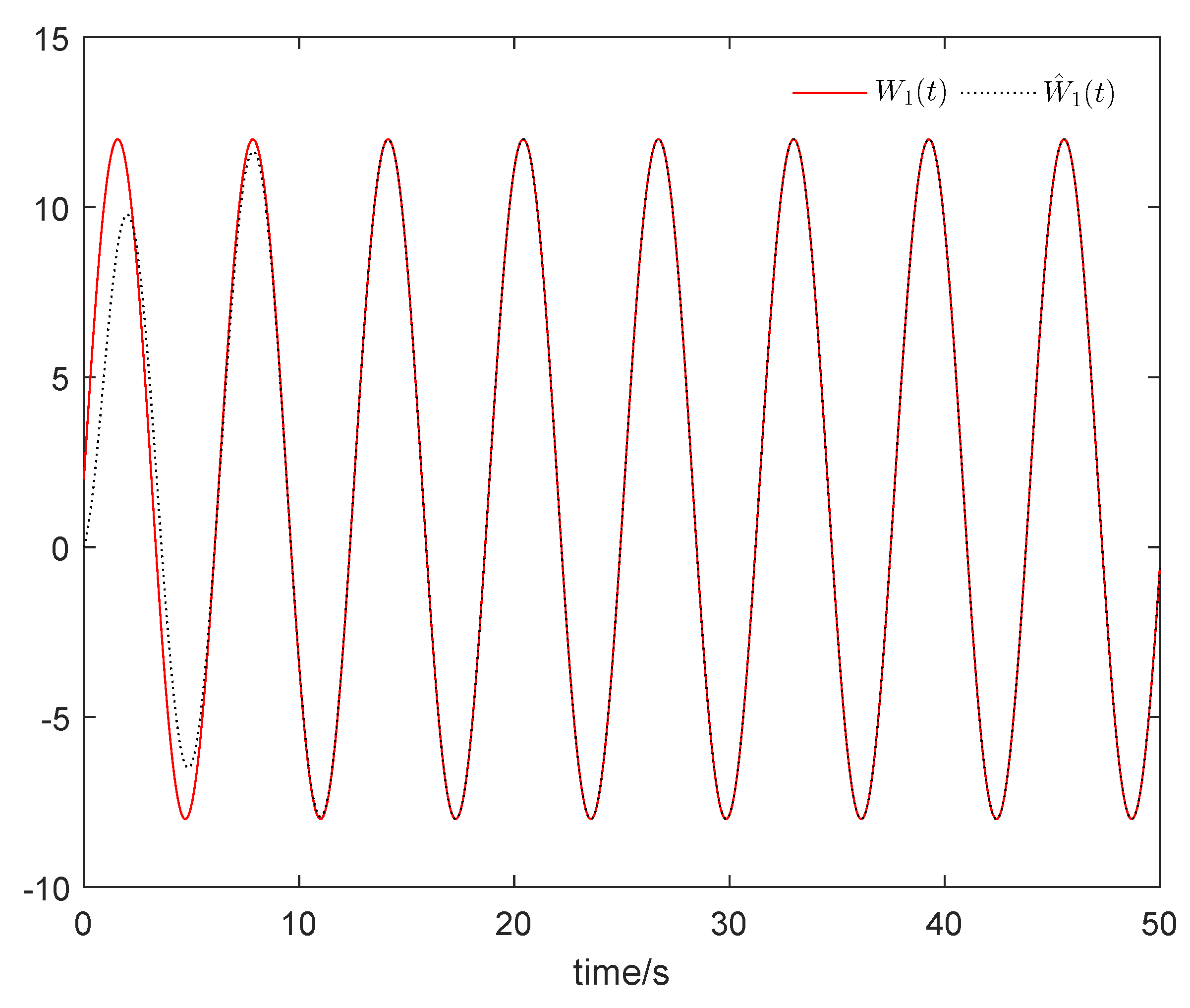
3.3. A Suitable Filter Is Designed for the Periodically External Disturbance

Theorem 4.

For the periodically external disturbance $W_1\left(t\right)=Asin\left(t\right)+C$, a suitable filter $G_f\left(s\right)$ is presented as follows

$$\begin{array}{c}\hfill G_f\left(s\right)=\frac{s^4+4s^3+6s^2+3s+2}{s^5+4s^4+8s^3+9s^2+6s+2}\end{array}$$

(25)

where $G_f\left(s\right)=\ell \left\{g_f\left(t\right)\right\}$,

$$\begin{array}{c}\hfill g_f\left(t\right)=2e^{-t}-e^{-t}(cos\left(t\right)-3sin\left(t\right))-\frac{4\sqrt{3}}{3}{e}^{-\frac{t}{2}}sin\left(\frac{\sqrt{3}t}{2}\right)\end{array}$$

(26)

and meets the following performance:

$${\widehat{W}}_1\left(t\right)=W_1\left(t\right)*{\ell }^{-1}\left[G_f\left(s\right)\right]=W_1\left(t\right)*g_f\left(t\right)\to W_1\left(t\right),ast\to \infty ,$$

(27)

“ℓ” represents the Laplace transform, “${\ell }^{-1}$” represents the inverse Laplace transform, “*” represents the convolution.

The proof of Theorem 4, please see Appendix A.4.

3.4. The DE-Based Controller Is Designed for Periodically External Disturbance

Theorem 5.

For the sum system (21), the DE-based controller $U_w$ is presented as follows

$$\begin{array}{c}\hfill U_w=B^{+}\left\{{\ell }^{-1}\left[\frac{G_f\left(s\right)}{1-G_f\left(s\right)}\right]*F\left(Z\right)-{\ell }^{-1}\left[\frac{s{G}_f\left(s\right)}{1-G_f\left(s\right)}\right]*E\right\},\end{array}$$

(28)

where $B^{+}={\left(B^{T}B\right)}^{-1}{B}^T$, $F\left(Z\right)=M\left(Z\right)+B{U}_s$.

The proof of Theorem 5, please see Appendix A.5.

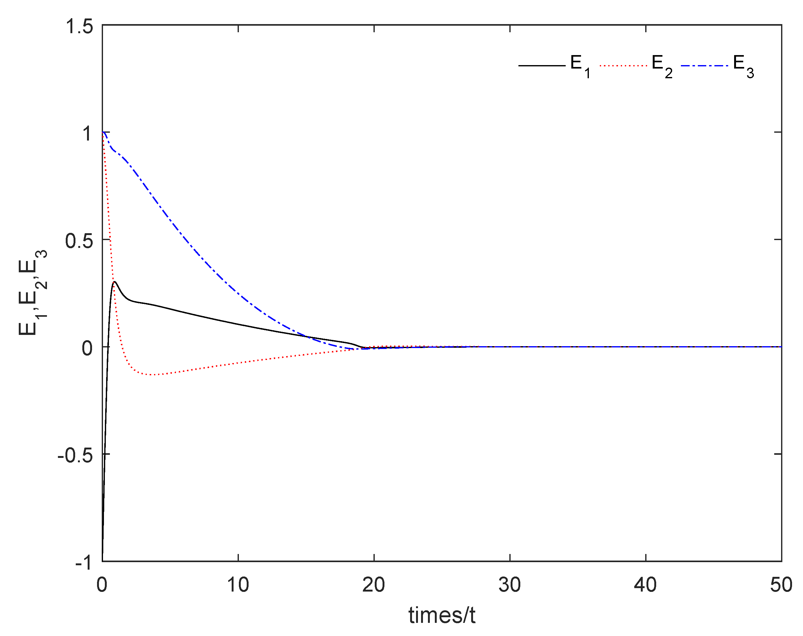
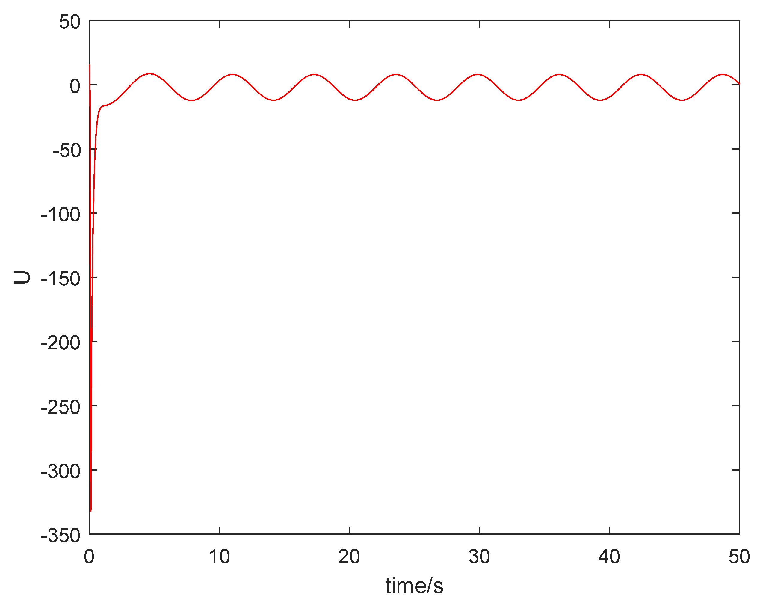
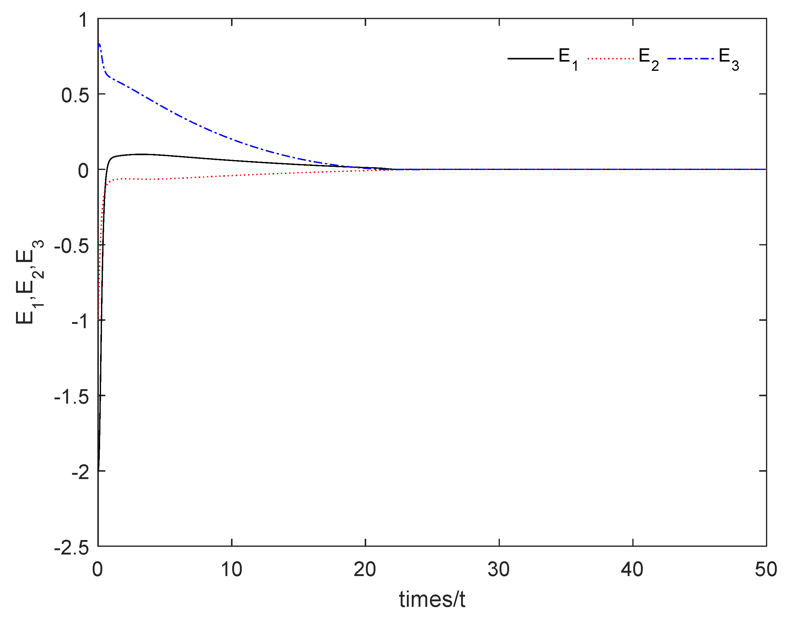
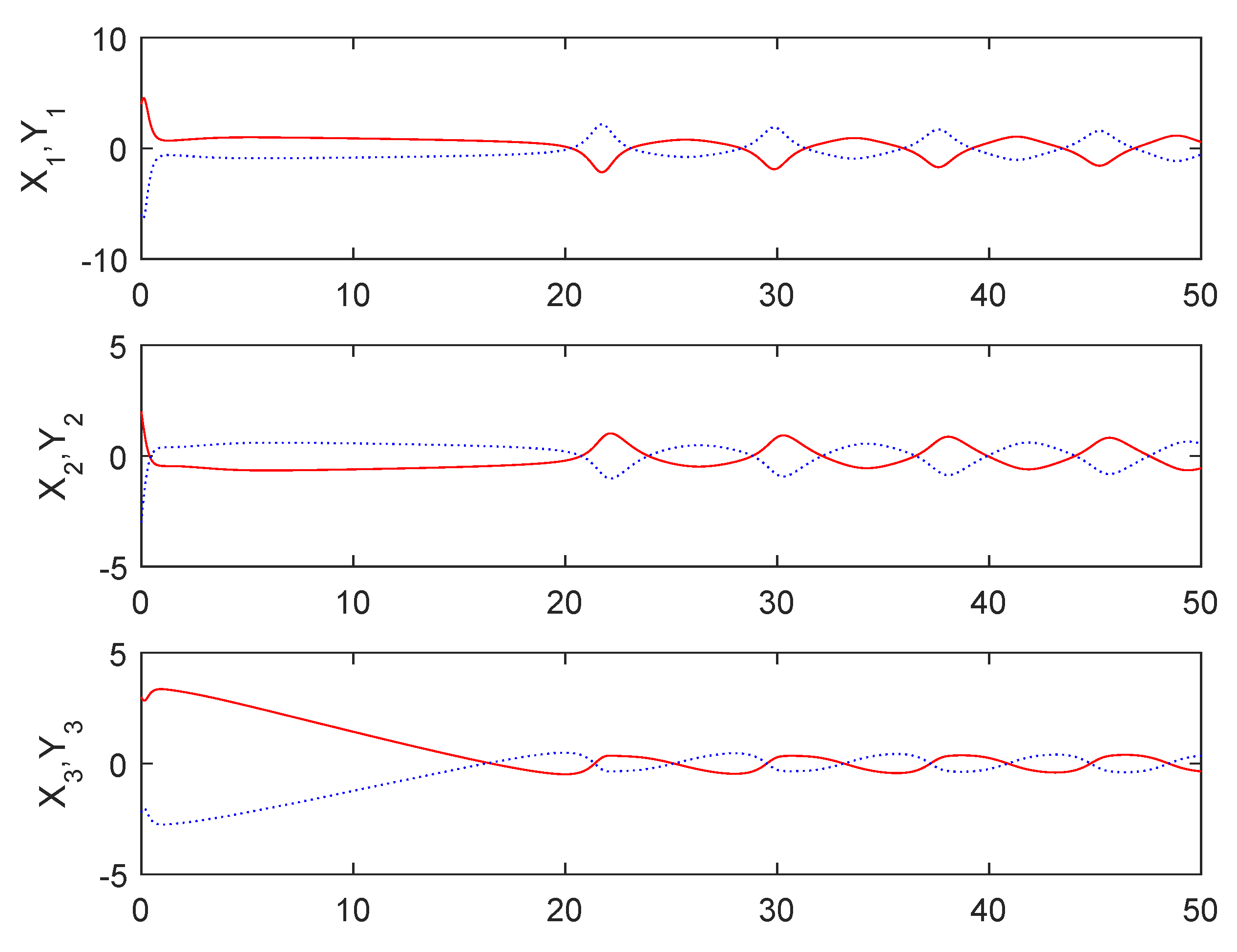
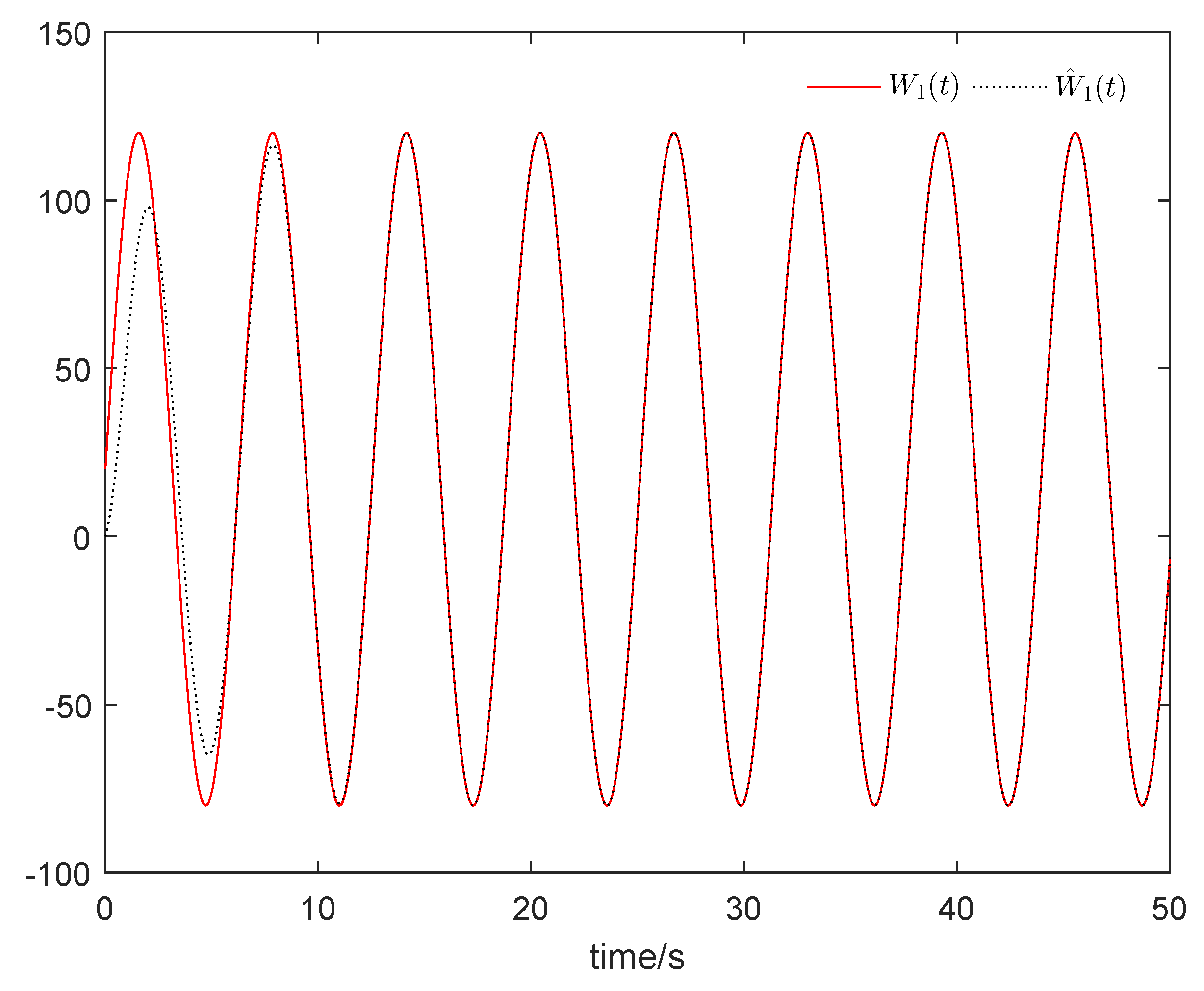
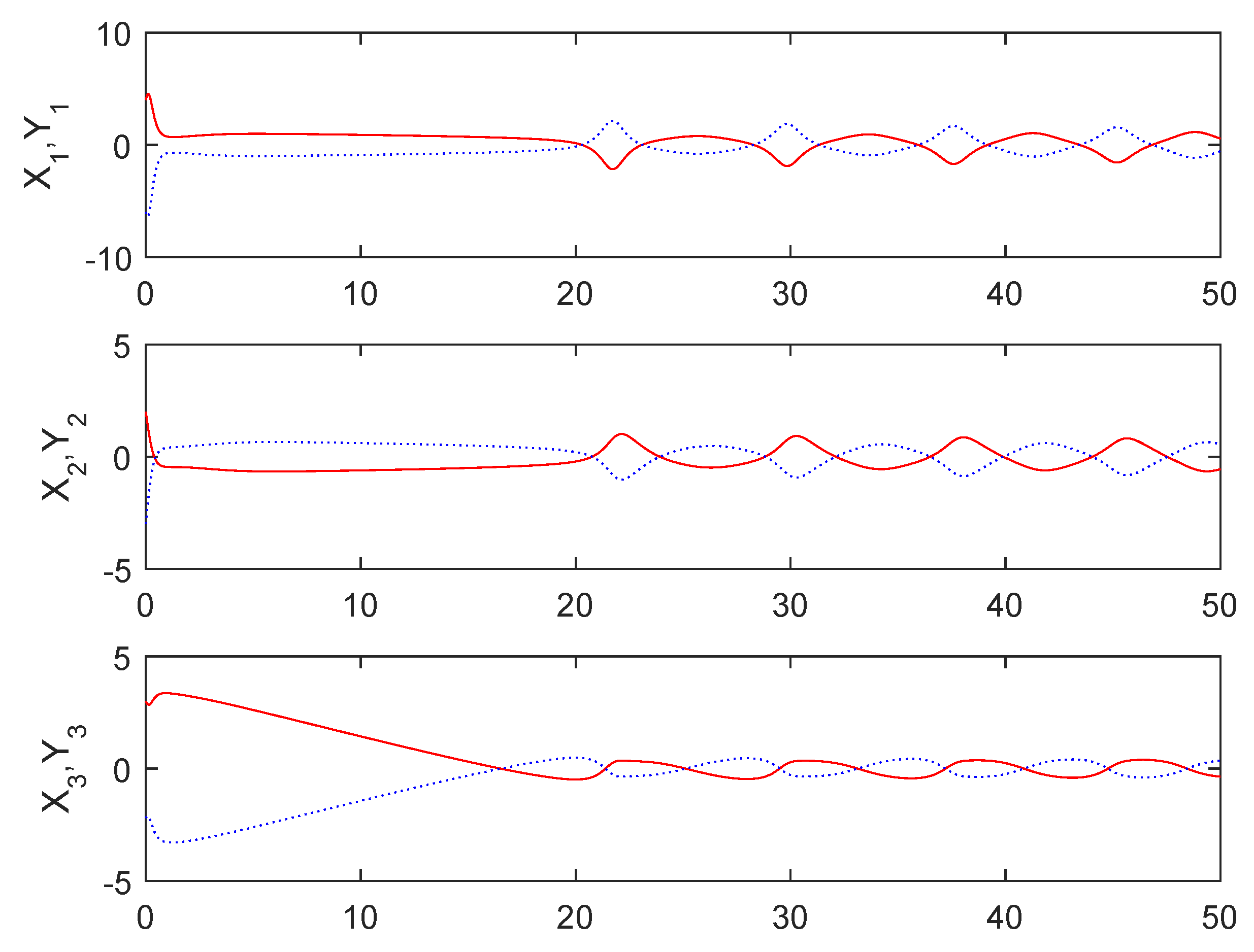
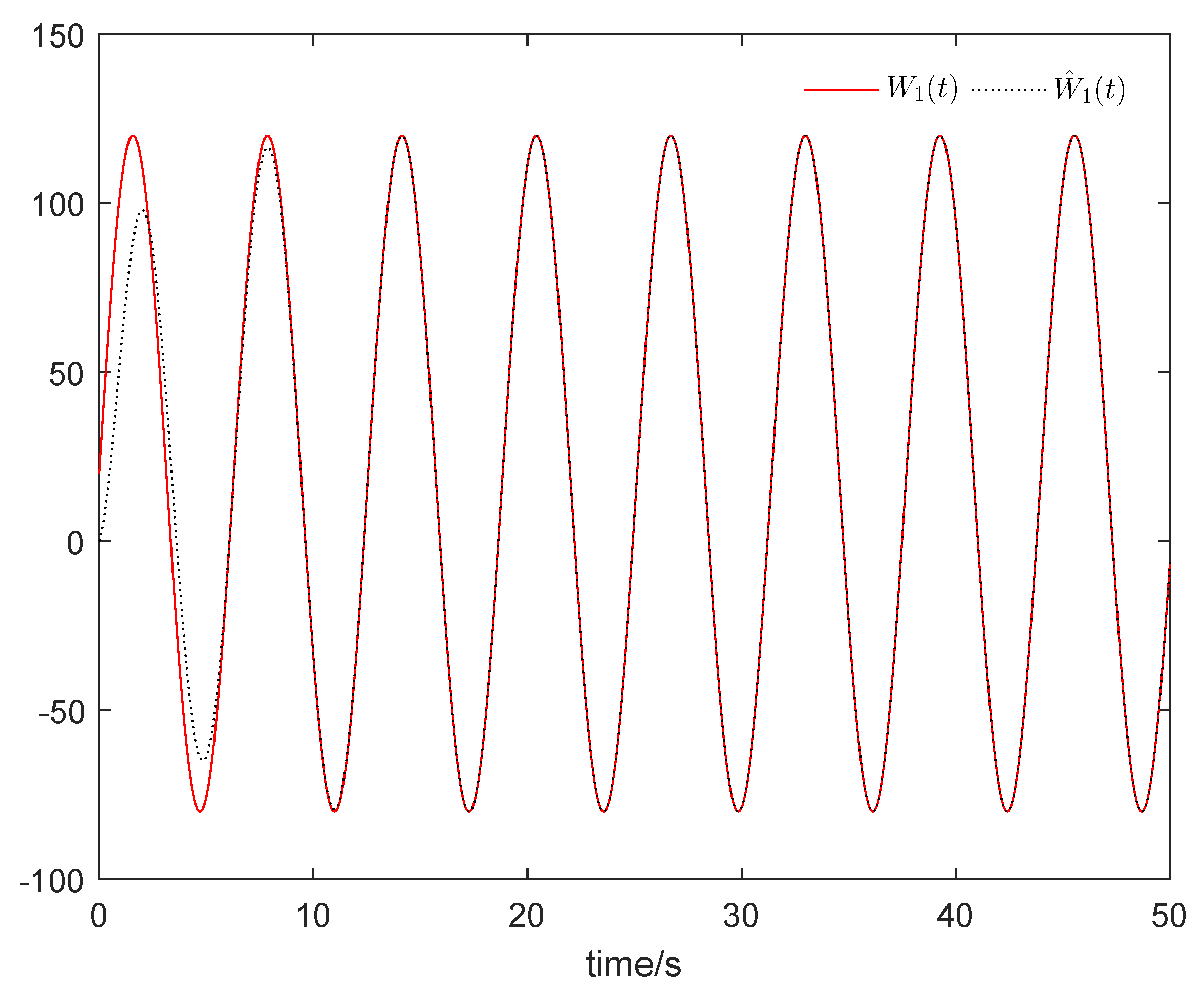
4. Numerical Simulation

4.1. Comparison with the Effect of Parameters of Periodically External Disturbance

The initial conditions of the master subsystem given in Equation (18) and the slave subsystem given in Equation (20) are chosen as $X\left(0\right)=[1,2,3],Y\left(0\right)=[-2,-1,-2]$, respectively, and $Z\left(0\right)=1$. Without loss of generality, the controller $U_s$ given in Equation (24) is taken as an example.

Case 1: $A=10,C=2$.

From Figure 1, it can be seen that the sum system is asymptotically stable. Figure 2 shows the states of the master subsystem and the slave subsystem, respectively. It is easy to see that the state vectors of the slave subsystem have the same amplitude but opposite signs to those of the master subsystem, which implies that the partial anti-synchronization problem of the 4D financial hyper-chaotic system is realized. Figure 3 shows that ${\widehat{W}}_1\left(t\right)$ tends to $W_1\left(t\right)$ as $t\to +\infty$. Figure 4 shows the state of control signal $U\left(t\right)$.

Case 2: $A=100,C=20$.

Figure 5 shows that the sum system is asymptotically stable. Figure 6 shows the states of the master subsystem and the slave subsystem, respectively. It is easy to see that the state vectors of the slave subsystem have the same amplitude but opposite signs to those of the master subsystem, which implies that the partial anti-synchronization problem of the 4D financial hyper-chaotic system is realized. Figure 7 shows that ${\widehat{W}}_1\left(t\right)$ tends to $W_1\left(t\right)$ as $t\to +\infty$. Figure 8 shows the state of control signal $U\left(t\right)$.

Remark 1.

From the above figures, it can be seen that the effect of the disturbance parameters (A and C) on the anti-synchronization problem is very small.

4.2. Comparison with the Same Control Strategy

The initial conditions of the master subsystem given in Equation (18) and the slave subsystem given in Equation (20) are chosen as $X\left(0\right)=[1,2,3],Y\left(0\right)=[-2,-1,-2]$, respectively, and $Z\left(0\right)=1$, and $A=100,C=20$. The controller $U_s$ given in Equation (24) is chosen here.

Figure 9 shows that the sum system is asymptotically stable. Figure 10 shows the states of the master subsystem and the slave subsystem, respectively. It is easy to see that the state vectors of the slave subsystem have the same amplitude but opposite signs to those of the master subsystem, which implies that the partial anti-synchronization problem of the 4D financial hyper-chaotic system is realized. Figure 11 shows that ${\widehat{W}}_1\left(t\right)$ tends to $W_1\left(t\right)$ as $t\to +\infty$. Figure 12 shows the state of control signal $U\left(t\right)$.

Remark 2.

From the above figures, it can be seen that the effect of the controller $U_s$ given in Equation (24) is stronger than that given in Equation (22).

5. Conclusions

The partial anti-synchronization problem of the 4D financial hyper-chaotic system with periodically external disturbance has been investigated. Firstly, the partial anti-synchronization problem of the nominal 4D financial system has been proven. Then, by designing a suitable filter, two disturbance estimator (DE)-based controllers have been presented and used to realize the partial anti-synchronization problem. It has been proven that the proposed filter can asymptotically estimate the periodically external disturbance. Finally, the effectiveness and correctness of the proposed results have been verified by numerical simulation.

References

1. Pecora, L.M.; Carroll, T.L. Synchronization in chaotic system. Phys. Rev. Lett. 1990, 64, 821–825. [Google Scholar] [CrossRef] [PubMed]
2. Mainieri, R.; Rehacke, J. Projective synchronization in three-dimensional chaotic oscillators. Phys. Rev. Lett. 1999, 82, 3042–3045. [Google Scholar] [CrossRef]
3. Xu, D.L. Control of projective synchronization in chatic system. Phys. Rev. Lett. 2001, 63, 027201–027204. [Google Scholar]
4. Park, J.H. Adaptive synchronization of Rossler system with uncertain parameters. Chaos Solitons Fractals 2005, 25, 333–338. [Google Scholar] [CrossRef]
5. Jiang, C.; Zhang, F.; Li, T. Synchronization and anti-synchronization of N-coupled fractional-order complex systems with ring connection. Math. Methods Appl. Sci. 2018, 41, 2625–2638. [Google Scholar] [CrossRef]
6. Karimov, A.; Tutueva, A.; Karimov, T.; Karimov, T.; Druzhina, O.; Butusov, D. Adaptive generalized synchronization between circuit and computer implementations of the Róssler system. Appl. Sci. 2021, 11, 81. [Google Scholar] [CrossRef]
7. Li, R.H.; Xu, W.; Li, S. Anti-synchronization on autonomous and non-autonomous chaotic systems via adaptive feedback control. Chaos Solitons Fractals 2009, 40, 1288–1296. [Google Scholar] [CrossRef]
8. Shi, J.C.; Zeng, Z.G. Anti-synchronization of delayed state-based switched inertial neural networks. IEEE Trans. Cybern. 2021, 51, 2540–2549. [Google Scholar] [CrossRef]
9. Lu, W.L.; Chen, T.P. QUAD-condition, synchronization, consensus of multiagents, and anti-synchronization of complex networks. IEEE Trans. Cybern. 2021, 51, 3384–3388. [Google Scholar] [CrossRef]
10. Wang, Q.; Duan, L. Finite-time anti-synchronisation of delayed Hopfield neural networks with discontinuous activations. Int. J. Control. 2021, 20, 2398–2405. [Google Scholar] [CrossRef]
11. Khan, T.; Chaudhary, H. Adaptive controllability of microscopic chaos generated in chemical reactor system using anti-synchronization strategy. Numer. Algebra Control. Optim. 2021, 12, 611–620. [Google Scholar] [CrossRef]
12. Wei, X.F.; Zhang, Z.Y.; Lin, C.; Chen, J. Synchronization and anti-synchronization for complex-valued inertial neural networks with time-varying delays. Appl. Math. Comput. 2021, 403, 126194. [Google Scholar] [CrossRef]
13. Kaheni, H.R.; Yaghoobi, M. A new approach for security of wireless sensor networks based on anti-synchronization of the fractional-order hyper-chaotic system. Trans. Inst. Meas. Control. 2021, 43, 1191–1201. [Google Scholar] [CrossRef]
14. Guo, R.; Qi, Y. Partial anti-synchronization in a class of chaotic and hyper-chaotic systems. IEEE Access 2021, 9, 46303–46312. [Google Scholar] [CrossRef]
15. Zhu, L.; Chen, Z. Robust input-to-output stabilization of nonlinear systems with a specified gain. Automatica 2017, 84, 199–204. [Google Scholar] [CrossRef]
16. Casau, P.; Mayhew, C.G.; Sanfelice, R.G.; Silvestre, C. Robust global exponential stabilization on the n-dimensional sphere with applications to trajectory tracking for quadrotors. Automatica 2019, 110, 108534. [Google Scholar] [CrossRef]
17. Ren, B.; Zhong, Q.; Chen, J. Robust control for a class of nonaffine nonlinear systems based on the uncertainty and disturbance estimator. IEEE Trans. Ind. Electron. 2015, 62, 5881–5888. [Google Scholar] [CrossRef]
18. Wang, Y.; Ren, B.; Zhong, Q. Robust power flow control of grid-connected inverters. IEEE Trans. Ind. Electron. 2016, 63, 6887–6897. [Google Scholar] [CrossRef]
19. Ren, B.; Zhong, Q.; Dai, J. Asymptotic reference tracking and disturbance rejection of UDE-based robust control. IEEE Trans. Ind. Electron. 2017, 64, 3166–3176. [Google Scholar] [CrossRef]
20. Ren, B.; Wang, Y.; Zhong, Q. UDE-based control of variable-speed wind turbine systems. Int. J. Control. 2017, 90, 121–136. [Google Scholar] [CrossRef]
21. Wang, Y.; Ren, B. Fault ride-through enhancement for grid-tied PV systems with robust control. IEEE Trans. Ind. Electron. 2018, 65, 2302–2312. [Google Scholar] [CrossRef]
22. Yi, X.; Guo, R.; Qi, Y. Stabilization of chaotic systems with both uncertainty and disturbance by the UDE-Based Control Method. IEEE Access 2020, 8, 62471–62477. [Google Scholar] [CrossRef]
23. Wang, Y.; Ren, B.; Zhong, Q. Bounded UDE-Based controller for input constrained systems with uncertainties and disturbances. IEEE Trans. Ind. Electron. 2021, 68, 1560–1570. [Google Scholar] [CrossRef]
24. Wu, W.; Chen, Z. Hopf bifurcation and intermittent transition to hyperchaos in a novel strong four-dimensional hyperchaotic system. Nonlinear Dyn. 2010, 60, 615–630. [Google Scholar] [CrossRef]
25. Yu, H.; Cai, G.; Li, Y. Dynamic analysis and control of a new hyperchaotic finance system. Nonlinear Dyn. 2012, 67, 2171–2182. [Google Scholar] [CrossRef]
26. Cai, G.; Hu, P.; Li, Y. Modified function lag projective synchronization of a financial hyperchaotic system. Nonlinear Dyn. 2012, 69, 1457–1464. [Google Scholar] [CrossRef]
27. Cao, L. A four-dimensional hyperchaotic finance system and its control problems. J. Control. Sci. Eng. 2018, 4976380, 1–12. [Google Scholar] [CrossRef]
28. Guo, R. Projective synchronization of a class of chaotic systems by dynamic feedback control method. Nonlinear Dyn. 2017, 90, 5593–5597. [Google Scholar] [CrossRef]
Figure 1. The sum system (21) is asymptotically stable.
Mathematics 10 03373 g001
Figure 2. The states of the master subsystem and the slave subsystem.
Mathematics 10 03373 g002
Figure 3. W ^ 1 ( t ) tends to W 1 ( t ) .
Mathematics 10 03373 g003
Figure 4. The state of control signal U ( t ) .
Mathematics 10 03373 g004
Figure 5. The sum system (21) is asymptotically stable.
Mathematics 10 03373 g005
Figure 6. The states of the master subsystem and the slave subsystem.
Mathematics 10 03373 g006
Figure 7. W ^ 1 ( t ) tends to W 1 ( t ) .
Mathematics 10 03373 g007
Figure 8. The state of control signal U ( t ) .
Mathematics 10 03373 g008
Figure 9. The sum system (21) is asymptotically stable.
Mathematics 10 03373 g009
Figure 10. The states of the master subsystem and the slave subsystem.
Mathematics 10 03373 g010
Figure 11. W ^ 1 ( t ) tends to W 1 ( t ) .
Mathematics 10 03373 g011
Figure 12. The state of control signal U ( t ) .
Mathematics 10 03373 g012
Publisher’s Note: MDPI stays neutral with regard to jurisdictional claims in published maps and institutional affiliations.