Fluctuation Analysis of a Soft-Extreme Shock Reliability Model

Abstract

In this paper, we deal with a mixed reliability system decaying from natural wear, occasional soft and hard shocks that eventually lead the system to failure. The aging process alone is linear and it is escalated through soft shocks such that they lead to the system’s soft failure when the combined damage exceeds a threshold M. The other threat is that posed by occasional hard shocks. When the total number of them identified as critical (each critical shock exceeds a fixed threshold H) reaches N, the system becomes disabled. With $N=1$, a critical shock is extreme. The arrival stream of shocks is a renewal process marked by soft and hard shocks. We establish a formula for a closed form functional containing system’s time-to-failure, the state of the system upon its failure, and other useful statistical characteristics of the system using and embellishing fluctuation analysis and operational calculus. Special cases provide tame expressions that are computed and validated by simulation.

1. Introduction

1.1. Background

A basic shock reliability system includes a complex device subject to continuous degradation (or aging or decay) due to natural wear. The system becomes inoperative when its key function is disabled. This can be specified through a real-valued degradation process $Y\left(t\right)$ and a sustainability threshold M that $Y\left(t\right)$ crosses sooner or later.

In addition, the system is assaulted at random times $t_1,t_2,\dots$ by shocks of random magnitudes $X_1,X_2,\dots$ that accelerate the system wear. It is likely that the system’s operation gets compromised due to one of such shocks sooner than system’s natural aging. Furthermore, the impact of the shocks can be felt on some other components of the system in the form of $Y_1,Y_2,\dots$

It stands for reason to interpret such system by a series of two (or more) components, so that the fatality of any of them deactivates the entire device. In a nutshell, the system natural wear represented by process $Y\left(t\right)$ is intertwined with $X_1,X_2,\dots$ referred to as soft shocks that accelerate the overall aging. The latter is formalized by the continuous time parameter process

$$\begin{array}{c}\hfill S\left(t\right)=Y\left(t\right)+\sum _{n=0}^{\infty }{X}_n{𝟙}_{[0,t]}\left(t_n\right),\end{array}$$

where ${𝟙}_A$ is the indicator function of a set A. Thus, the system “perishes” if its first component completely deteriorates through $S\left(t\right)$ crossing M at some time t. Its second component is stricken by hard shocks $W_1,W_2,\dots$ at the same times $t_1,t_2,\dots$ as soft shocks $X_1,X_2,\dots$ hit the first component. So the second component can be knocked down by one such hard shock that also disables the system. Now the system can fend off itself of most such dangerous attacks with no damage. However, one such hard shock can become fatal to the system if it is stronger than the system can handle. More specifically, a hard shock $W_k$ is fatal to the system if $W_k>H$ (a fixed threshold). An embellished variant of this scenario is when only after the component is hit by $N(\ge 1)$ such shocks does the system fail. In such case, the associated hard shocks are called critical. When $N=1$, a critical shock is called extreme.

One can think of an electrical system, under occasional surges, that is being relatively safe under the protection of a surge guard. However, one or several such surges can circumvent the guard not only by knocking it down but severely damaging the electrical grid that will require a substantial repair or be beyond repair. As mentioned, a single fatal hard shock is also referred to as an extreme shock and an associated reliability model is called an extreme shock model. Yet with N hard shocks needed to incapacitate the system, all are referred to as critical and the corresponding model is referred to as N-critical shock model.

There are different terminologies in the reliability literature, often synonymous. We would like to bring at least some of them together, along with other terms borrowed from fluctuation theory, and apply them to a generic serial system of two components. Hence, the system fails when so does at least one of its two components. Now the system we will deal with is as follows.

• The system ages according to an affine or linear deterministic process $Y\left(t\right)=Y\left(0\right)+at,$ $a>0$ is a constant slope.
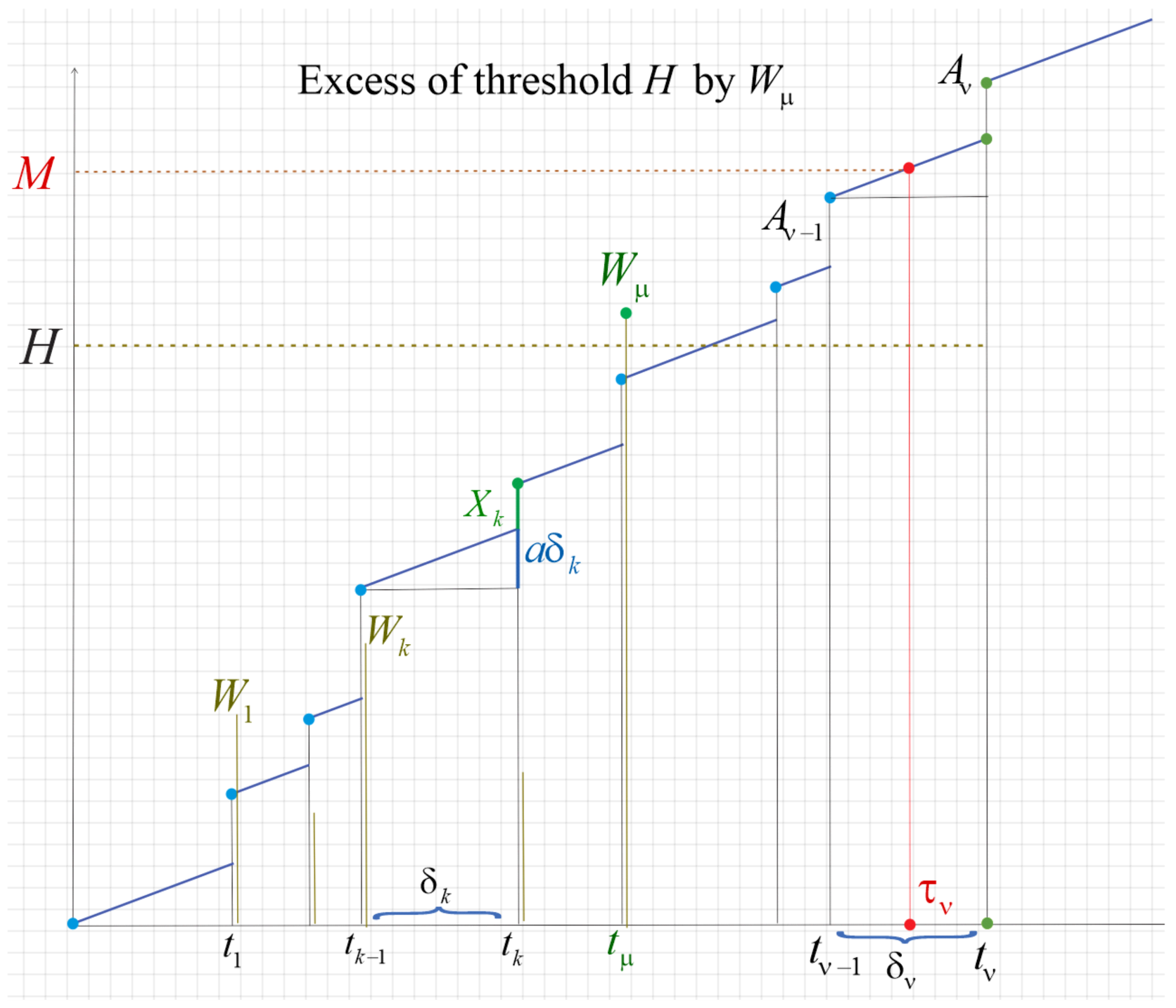
• Component 1 is periodically hit by soft shocks at times $t_1,t_2,\dots$ of magnitudes $X_1,X_2,\dots$ whose impact is cumulative. The latter means that every soft shock will escalate the wear of the device until its total damage combined with aging will top sustainability threshold M. The associated continuous time parameter process $S\left(t\right)$ describing the fatigue of the system at time $t\ge 0$ is

  $$\begin{array}{c}\hfill S\left(t\right)=Y\left(t\right)+\sum _{n=0}^{\infty }{X}_n{𝟙}_{\left[0,t\right]}\left(t_n\right)=Y\left(0\right)+at+\sum _{n=0}^{\infty }{X}_n{𝟙}_{\left[0,t\right]}\left(t_n\right),\end{array}$$

  where ${𝟙}_A$ is the indicator function of a set A. Component 1 and thus the system fails when one of two events occurs:

  (a)

  $S\left(t\right)=M$ at some t while $S\left(u\right)<M$ for all $u<t$ called a wear failure

  (b)

  $S\left(t_k\right)\ge M$, while $S\left(t\right)<M$ for all $t<t_k,$ called cumulative failure

  Either type of failure is called soft. Note that if $S\left(t_k\right)\ge M$ while $S\left(t\right)<M$ for $t<t_k,$ shock $X_k$ is called fatal. The first $k-1$ shocks $X_1,\dots ,X_{k-1}$ are then nonfatal.
• Component 2 is hit by hard shocks at the same times $t_1,t_2,\dots ,$ but with different upshots. Assume that those shocks hitting Component 2 with their respective magnitudes $W_1,W_2,\dots$ normally cause no damage unless one of them exceeds a critical threshold H. In this case, it knocks the component and thus the system down representing an unsustainable surge. Obviously, such a hit is also fatal, but it is referred to as extreme. Once the system becomes inoperative through an extreme shock, its failure is called extreme failure (as opposed to the cumulative or wear failure of Component 1). It is also called a hard failure and we call the associated hard shocks to tell them from soft shocks. Consequently, not all hard shocks are fatal, just the one in excess of threshold H.
• As mentioned, an upgrade to the extreme failure model is an N-critical failure model, when its component breaks down after being hit by N critical shocks exerted in no particular order. A hard shock $W_k$ is critical if $W_k>H$. Thus, if after being hit $N+m$ times by $W_1,\dots ,W_{N+m},$ there are N critical shocks from among the total of $N+m$ shocks and $W_{N+m}>H,$ the system fails at time $t_{N+m}$ (unless it fails earlier for other reasons). This last shock becomes also fatal. More restrictively, if system’s failure requires all critical shocks to arrive sequentially, the corresponding model is called a run shock model.
• Because aging, soft and hard shocks compete with each other, we proceed with further formalism from fluctuation theory. Let

  $$\begin{array}{cc}\hfill & \nu =inf\left\{n:A_n=\sum _{k=1}^n(X_k+a{\delta }_k)\ge M\right\}\hfill \\ & \mu =inf\{m:W_m>H\}\hfill \\ & \rho =\nu \wedge \mu \hfill \end{array}$$
  Then, $\rho$ is the shock failure index. As mentioned, the system failure can occur even earlier at some time $t\in \left(t_{\rho -1},t_{\rho }\right)$ when $S\left(t\right)=M$ due to aging and accumulated shocks combined, but not due to a single shock (meaning it is a mere wear failure). It is convenient to combine the two situations in one using random time ${\tau }_{\rho }$ which is either $t_{\rho }$ or some $t\in \left(t_{\rho -1},t_{\rho }\right)$ when $S\left(t\right)=M$. The system is rendered inoperative at the time-to-failure being ${\tau }_{\rho }$ and consequently, the exit from its operational mode can be regarded as the end of a game of “three players” often alluded so in the literature by referring it to as a competition of several failure processes. Note that ${\tau }_{\rho }$ is also referred to as the lifetime of the system. So, in a nutshell, ${\tau }_{\rho }$ is the time-to-failure, or lifetime of the system, or also the first passage time of the combined aging, cumulative, and extreme failure process.
• The above-mentioned N-critical failure model is more convenient to describe by an auxiliary sequence $Y_1,Y_2,\dots$ of binary r.v.’s (random variables) defined as $Y_k={𝟙}_{\left\{W_k>H\right\}}$. So the $\mu$-index is then $\mu =inf\left\{m:{\sum }_{i=1}^m{Y}_i=N\right\}$ with the rest identical to that in 5.

In this paper, we target the following characteristics that we deem imperative in the statistical assessment of our system. We verbalize them in this section and then state the problem rigorously in Section 2. We predict the life time of the system and the detriment of the damage to either component upon the exit. Furthermore, we also predict the pre-failure time $t_{\rho -1}$ and status of the system $S\left(t_{\rho -1}\right)$ at time $t_{\rho -1}$. This information can help take preventive measures ahead of the exit at ${\tau }_{\rho }$ or $t_{\rho }$.

Many authors cited below investigate similar systems, but they use different techniques and many target various probabilistic characteristics of underlying systems. We will mention how they relate to our work. The most common term for our model and many similar models is a mixed reliability system. In a nutshell, such classes of mixed reliability systems include aging, typically continuous aging driven by a stochastic process (like gamma or Brownian motion) or a linear process $Y\left(t\right)=at$, where slope a is a random variable. The system is hammered by a bivariate marked Poisson process of shocks $\left(X_k,W_k\right)$ arriving at $t_1,t_2,\dots$ and forming an ordinary or nonhomogeneous Poisson point process. Marks $\left(X_k,W_k\right)$ can be position $\left(t_k\right)$-dependent or position-independent. The marks themselves $\left(X_k,W_k\right)$ are most often independent of each other. The marked process of shocks can also be general renewal (as it is the assumption in our paper) and with position-dependent marking or as complex as a Markov renewal process.

1.2. Relevant Work

Cha and Finkelstein [1] in 2011 studied a mixed model with cumulative and extreme shocks, non-homogeneous Poisson process of shocks, and no ageing. Each shock at time t is fatal or not fatal with probabilities $p\left(t\right)$ and $1-p\left(t\right),$ respectively. Other setting is the critical shocks become fatal when their total number exceeds N. N can also be random.

In 2021, Bian et al. [2] considered a multi-component system subject to competing failure processes, so that the degradation function of the ith component is

$$\begin{array}{c}\hfill S_i\left(t\right)=Y_i\left(0\right)+a_{i}t+\sum _{k=0}^{\infty }{X}_k^{\left[i\right]}{𝟙}_{\left[0,t\right]}\left(t_k\right),\end{array}$$

where the slope $a_i$ is a Gaussian r.v. Besides, the ith component is also hit by hard shocks $W_k^{\left[i\right]};k=1,2,\dots ,$ and it is knocked down when one of them exceeds $H_i$. The hard shocks form a nonhomogeneous Poisson point process with multivariate marks.

Cao et al. [3], in their 2020 paper, studied an aging system under soft and hard shocks arriving in accordance with an ordinary Poisson process with a constant rate. Cumulative aging is integrated with internal shocks and degradation $S\left(t\right)=Y\left(t\right)+{\sum }_{k=0}^{\infty }{X}_k{𝟙}_{\left[0,t\right]}\left(t_k\right)$. The extreme failure threshold is time-dependent.

In 2022, Che et al. [4] studied a system under natural aging (machine degradation), soft shocks (human errors), and hard shocks arriving according to a Poisson process.

In 2021, Li et al. [5] proposed an interesting mixed system that can be applied to satellites or various spacecraft. The lifetime of the phased mission systems can be separated into several phases, in which their tasks, system configurations, and failure criteria are different. Shocks are due to radiation from outer space and they cause an additional wear and fatal damage to electronic devices in these systems. The authors modeled the system by a Markov regenerative process. More specifically, the self-wear linear process is $Y\left(t\right)=at$ ($a\in \left[N\left(\mu ,{\sigma }^2\right)\right]$), additional wear is cumulative driven by iid (independent and identically distributed) Gaussian r.v.’s, external damages (extreme) are due to iid Gaussian r.v.’s. Both are independent. Shocks follow an ordinary Poisson process.

In 2021, Lyu et al. [6] modeled a mechanical system with degradation, soft and hard shocks under a linearly decreasing threshold.

In 2020, Meango and Ouali [7] studied a mixed system with cumulative and extreme failures. Shocks arrive according to a Poisson process.

In 2014, Mercier and Pham [8] studied a variant of hard shocks that are fatal or not fatal by means of Bernoulli trials rather than in association with threshold’s crossings. The system carried aging and soft shocks and all three competed with each other. The authors offered the interpretation of a two-component serial system as in our description above. The lifetime of the first component is characterized by its intrinsic hazard rate, whereas the wear of the second component—by a gamma process. The lifetimes of the two components are dependent through a nonhomogeneous Poisson process of shocks. A shock is fatal with probability $p\left(t\right)$ and with probability $1-p\left(t\right)$ it is nonfatal. The authors calculated the system reliability.

In 2018, Peng et al. [9] introduced a generalized extreme shocks reliability system where shocks increase the degradation rate when their values exceed a critical threshold. The aging process involves Brownian motion process.

In 2020, Wang et al. [10] considered an interesting applied reliability system with aging and a shock process motivated by the wear process of a micro engine of micro electromechanical system. The failure is manifested by the visible wear of the rubbing surfaces between the gear and the pin joint modeled by a linear degradation path model. The wear is primarily caused by the mechanism’s aging, while shock tests on micro engine reveal that shock loadings may cause substantial wear debris among the gear, the pin joint, and the fracture of springs. The micro engine fails if the shock imposed on it exceeds a critical value. In this sense, shocks were produced by the external environment, and their arrival rate was not affected by the degradation state. As the wear accumulates, the micro engine becomes more vulnerable and its resistance to shocks decreases. Therefore, the thresholds for distinguishing shocks in safety zone, damage zone, and fatal zone had to be decreased accordingly.

The natural wear is modeled by $Y\left(t\right)=at$, where a is a r.v.—the rate for the degradation path. Shocks arrive according to a Poisson process $N\left(t\right)$ with rate $\lambda$. They are divided into safety, damage, and fatal zones according to their random magnitudes $W_i$, ($i=1,2,\dots$). If the magnitude of a shock is below the safety threshold $H_s$, the shock does not affect the natural degradation progression. If the magnitude of a shock is beyond the fatal threshold $H_f>H_s$, it will cause a failure immediately. And a shock with its magnitude between these two thresholds will bring cumulative damage to the natural degradation process. Altogether, the system modeled by a combination of an aging process and shocks identified as harmless, soft, and extreme depending on their position within the three zones induced by $H_s<H_f$.

A somewhat analogous setting was rendered earlier in Eryilmaz [11] in 2015. A system is hit by random shocks. Let $c_1$ and $c_2$ be two critical thresholds such that $c_1<c_2$. A shock with a magnitude between $c_1$ and $c_2$ causes a partial damage to the system, and the system moves into a lower partially working state decreased by one unit upon the occurrence of each shock in ($c_1,c_2$). A shock with a magnitude above $c_2$ is extreme and causes a complete failure. Such a shock model creates a multi-state system having random number of states. The authors target the lifetime, the time spent by the system in a perfect functioning state, and the total time spent by the system in partially working states along with their survival functions. The interarrival times between successive shocks follow phase-type distribution.

In 2021, Wu et al. [12] studied an N-critical shock model. The critical shocks $\left\{W_k\right\}$ arrive in accordance with a semi-Markov process and Markov-dependent arrival process $\left\{t_k\right\}$. Recall that a shock is critical if it crosses some H. The system fails if the total number of critical shocks reaches N. The time-to-failure of the system which is the time from 0 to the Nth critical shock is targeted.

Yousefi et al. [13] in 2019, studied a series system with n components, each subject to degradation and hard shocks. The magnitudes of shocks exerted to each particular component are iid Gaussian r.v.’s. The shocks arrive simultaneously to all components according to a marked Poisson process $\mathcal{S}={\sum }_{j=1}^{\infty }\left(X_j^1,\dots ,X_j^n\right){\epsilon }_{t_j}$ of rate $\lambda$ and its support counting measure ${\sum }_{j=1}^{\infty }{\epsilon }_{t_j}$ with position-independent marking. The system ages according to the gamma process $Y\left(t\right)$ with shape parameter $\alpha \left(t\right)$ and scale parameter $\beta$.

1.2.1. Other Relevant Shock Models

Most shock models fall into one of the five classes: cumulative shock models, extreme shock models, $\delta$-shock models, run shock models, and mixed shock models. A mixed shock model must be a combination of at least two of the first four types.

A $\delta$-shock model is of the system that fails when the time lag between two consecutive shocks becomes less than some $\delta >0$. $\delta$-shock policy is often implemented whenever shock damages are hard to observe.

In 2018, Hao and Yang [14] considered a system that fails due to a competition of soft and hard failures. Soft failure happens when the cumulative degradation along with soft shocks cross a critical threshold. A hard failure is modeled according to variable hard failure thresholds as a combination of extreme and $\delta$-shocks. The continuous degradation process $Y\left(t\right)$ is linear and shocks arrive following a homogenous Poisson process with a constant rate $\lambda$.

Kus et al. [15], in 2021, studied a mixed shock model which combines $\delta$-shock and extreme shock models considering a class of matrix-exponential distributions for inter shock times. The lifetime (time-to-failure) of the system does not have matrix-exponential distribution, but it is approximated by a matrix-exponential distribution. They also obtained the reliability function of the system.

1.2.2. Run Shock Models

Input of shocks is specified by a marked point process $\mathcal{S}={\sum }_{k=1}^{\infty }{X}_n{\epsilon }_{t_n}$, with ${\delta }_k$ being interarrival times of the shocks. Such a system was introduced and studied by Mallor and Omey [16] and Mallor and Santos [17], with the failure of the system defined as follows. Given a critical region$R\subseteq \mathbb{R}$, let $\nu \left(k\right)=min\left\{n:X_n,X_{n-1},\dots ,X_{n-k+1}\in R\right\}$ be a critical run in a string of k critical shocks that cause the failure of the system, with the failure time $t_{\nu \left(k\right)}$.

Eryilmaz and Tekin [18] considered a system with input of shocks being a marked point process with and without position dependence. They introduce two thresholds, $d_1<d_2$ such that

$$\begin{array}{cc}\mu =inf\left\{n:X_{n-k+1}>d_1,\dots ,X_n>d_1\right\}\hfill & \hfill \left(\mathrm{run}\mathrm{shock}\right)\\ \nu =inf\left\{n:X_n>d_2\right\}\hfill & \hfill \left(\mathrm{extreme}\mathrm{shock}\right)\\ \rho =\mu \wedge \nu \hfill & \end{array}$$

The failure time is $t_{\rho }$. No assumption is made on the nature of that point process. They found a closed formula for the probability distribution for $\rho$ having a phase type distribution, and for the special case of ${\delta }_n=t_n-t_{n-1}$ being of a phase type and the point process with position-independent marking, the failure time $t_{\rho }$ was proved to be of a phase type.

1.3. Studied Reliability System

In the present paper, our degradation process is linear or affine with a constant or random degradation rate, soft and N-critical soft shocks. (We discuss an embellishment of the system with N being random.) We allow the input process of shocks to be marked renewal with position-dependent marking. The present system is a weighty generalization of our recent 2021 paper that studied only a cumulative shocks and degradation system [19].

We study a rather general reliability system. It includes the natural wear and a bivariate marked renewal process of soft and critical shocks. All three attributes (aging, soft shocks, and critical shocks) lead to system’s failure. Most likely one of the three fatalities comes first and thus we can regard it as a game of three players, of which one wins the game when this player is the first to crash the system. We also relax our assumptions on critical shocks allowing N of them (rather than just one) to impair the system, where $N\in \mathbb{N}$. When $N=1$, a single critical shock is called extreme.

Furthermore, we employ a novel technique to solve the problem, namely an embellished variant of fluctuation analysis and discrete-continuous operational calculus developed in our earlier work [20,21,22]. It allowed us to obtain explicit analytic formulas that stay in contrast to other results that rely on algorithms or asymptotics. The key benefit of our method lies in its easier control implementation.

1.3.1. More Details on Used Techniques

Our techniques fall into the category of fluctuation theory in the context of random walk processes. However, our version of random walk is different from a classic one where a walker moves along a rectangular deterministic grid. There are none of these. First off, the grid is not rectangular, and secondly, it is random. The random walk (rather a doubly random walk) interpretation lies in its setting of the escape time ${\eta }_{\rho }$ from the bounded set $\mathcal{B}=(0,{\eta }_{\rho }]\times (0,M]\times (0,H]\subseteq {\mathbb{R}}^3$ and the position of the walker $\left({\eta }_{\rho },A_{\rho },B_{\rho }\right)$ upon escape from $\mathcal{B}$.

This is a novel model in the context of random walks and new identification of reliability models as random walks. Secondly, we apply and embellish the theory of fluctuations to arrive at analytically closed formulas for the main functional that carries the joint probability distribution of the first passage time and the position of walker or escape location associated with the failure time and the extent of the overall damage, respectively. Discrete-continuous operational calculus developed in our past work is a main feature of our method.

Note that estimating the time and excess level when crossing thresholds M and H by a bivariate piecewise constant jump process alone has been established in our past work on fluctuations of stochastic processes (Dshalalow [20] in 1997, Dshalalow [21] in 2005, and Dshalalow and White [22] in 2021), but its combination with the aging process poses more challenge. In the context of random walk, here the associated grid is not rectangular (nor is it deterministic). In 2021, Dshalalow and White [19] made one such step considering aging and soft-shocks process combined. In the present setting, there is yet another component representing critical shocks that need to hit the underlying device N times to knock it down. Our approach allows further embellishments by attaching other types of shocks.

1.3.2. Paper’s Layout

The paper is organized as follows. In Section 2, we formalize the system. We use and further develop fluctuation theory, along with operational calculus to obtain a closed form functional of the joint distribution of the time-to-failure and the detriment of the damage to the system, among other useful characteristics. To warrant our claim of closed-form expressions we reduce them to fully tractable special cases that we then compute, all in Section 3, and validate through simulation in Section 4.

2. Fluctuation Analysis of the Linear Degradation Process with Two Types of Shocks

Formal Description of the System

Consider a device that ages at a deterministic rate $a>0$, whose wear $Y\left(t\right)=Y\left(0\right)+at$ will render it inoperative when $Y\left(t\right)$ meets threshold M at time $t=\left(M-Y\left(0\right)\right)/a$. (We can also assume that a is a r.v. and this condition can be managed for special cases.) Without loss of generality we assume $Y\left(0\right)=0$. Otherwise, it will add just a little complexity to our analysis, even if $Y\left(0\right)$ is random.

The device degrades much faster through occasional irreversible damages due to soft shocks of random magnitudes $X_1,X_2,\dots$ arriving at random times $t_1,t_2,\dots$. These shocks can also fatally damage another component of the system. We assume that the impact of the shocks on the other component is manifested by a sequence $W_1,W_2,\dots$. Most of these shocks are harmless, but just one of them can be fatal. We call $\left\{W_k\right\}$ hard shocks. Their effect is binary with respect to a given threshold H, because with $W_k\le H,$ there is no impact felt on the system, but with $W_k>H,$ the whole system is knocked down.

In a nutshell, the system will fail when system’s fatigue defined by process

$$\begin{array}{c}\hfill S\left(t\right)=at+\sum _{k=1}^{\infty }{X}_k{𝟙}_{\left[0,t\right]}\left(t_k\right)\ge M\end{array}$$

(1)

crosses M or if $W_k>H$ at some epoch of time $t_k,$ whichever of the two comes first. The latter event is referred to as a hard failure due to the extreme shock $W_k$.

In Figure 1 is an excerpt of $S\left(t\right)$ alone in interval $\left[t_{k-1},t_k\right]$.

Denote

$$\begin{array}{c}\hfill A_n=\sum _{k=1}^n{X}_k+a{\delta }_k\mathrm{where}{\delta }_k=t_k-t_{k-1}\end{array}$$

(2)

and

$$\begin{array}{c}\hfill \nu =inf\left\{n\in \mathbb{N}:A_n\ge M\right\}\end{array}$$

(3)

Now the first crossing of threshold M can occur at $t_{\nu }$, and $A_{\nu }$ will most likely exceed M rather than attain to M. But because $S\left(t\right)$ is continuous in interval $\left(t_{\nu -1},t_{\nu }\right)$, crossing of M can also take place in this interval where $S\left(t\right)=M$ sharp. Yet the point t at which $S\left(t\right)$ assumes M is obviously random. So it makes sense to define the crossing point by ${\tau }_{\nu }$ as

$$\begin{array}{c}\hfill {\tau }_{\nu }=\left\{\begin{array}{cc}{t}_{\nu },& M\in (A_{\nu -1}+a{\delta }_{\nu },A_{\nu }]\\ t_{\nu -1}+\left(M-A_{\nu -1}\right)/a,& M\in (A_{\nu -1},A_{\nu -1}+a{\delta }_{\nu }]\end{array}\right.\end{array}$$

(4)

and call it the time-to-soft-failure. See Figure 2 and Figure 3 below.

The degradation of the system as observed upon times $\left\{t_k\right\}$ can be formalized by the marked random measure

$$\begin{array}{c}\hfill \mathcal{A}=\sum _{k=1}^{\infty }\left(X_k+a{\delta }_k\right){\epsilon }_{t_k},\end{array}$$

(5)

where ${\epsilon }_a$ is the unit measure with respect to a fixed point a.

Regarding the hard failure, we say the following. Because the impact of hard shocks is binary, we introduce an auxiliary sequence $Y_1,Y_2,\dots$ of r.v.’s,

$$\begin{array}{c}\hfill Y_i={𝟙}_{\left\{W_i>H\right\}}\end{array}$$

(6)

and

$$\begin{array}{c}\hfill B_k=\sum _{i=1}^k{Y}_i\end{array}$$

(7)

Then, obviously, the entire system fails when (at some $t_k$) $B_k=1,$ preceded by $B_1=0,\dots ,B_{k-1}=0$. The bivariate marked random measure reads as

$$\begin{array}{c}\hfill \mathcal{R}=\sum _{k=1}^{\infty }\left(X_k+a{\delta }_k,Y_k\right){\epsilon }_{t_k}\end{array}$$

(8)

The impact of hard shocks on the system is formalized as follows. Let

$$\begin{array}{c}\hfill \mu =inf\left\{m\in \mathbb{N}:W_m\ge H\right\}=inf\left\{m\in \mathbb{N}:Y_m=1\right\}\end{array}$$

(9)

Then, $t_{\mu }$ is the first passage time of process $\left\{B_m\right\}$, that is, $t_{\mu }$ is the time-to-hard-failure of the system without consideration of soft shocks and aging. Denote

$$\begin{array}{c}\hfill \rho =\nu \wedge \mu \end{array}$$

(10)

and call it the fatality index.

Below are some figures displaying different types of failures.

As can be seen in Figure 2, a wear failure takes place upon exact crossing of M by $S\left(t\right)$ before an extreme shock takes on the system.

Figure 3 depicts a variant of crossing (by exceeding) M at $t_{\nu }$ due to the $t_{\nu }$th soft shock $X_{\nu }$. This happens because $A_{\nu -1}+a{\delta }_{\nu }<M$ and with no intermediate crossing of M in interval $\left(t_{\nu -1},t_{\nu }\right)$.

Figure 4 exhibits an earlier crossing of threshold H through an extreme shock $W_{\mu }$ at an earlier moment $t_{\mu }$. The fatality index is thus $\rho =\mu$ and then $t_{\mu }$ turns to $t_{\rho }$.

As previously noted, the device under consideration consists of two separate components of which the first one is linearly decaying and under soft shocks, while the second one is subject to extreme shocks.

We denote by $S_{\nu }$ the soft state of the system upon its soft failure at time ${\tau }_{\nu }$:

$$\begin{array}{c}\hfill S_{\nu }=\left\{\begin{array}{cc}{A}_{\nu },& M\in (A_{\nu -1}+a{\delta }_{\nu },A_{\nu }]\\ M,& M\in (A_{\nu -1},A_{\nu -1}+a{\delta }_{\nu }].\end{array}\right.\end{array}$$

(11)

The hard failure time is $t_{\mu },$ when $B_{\mu }\ge N$ for the first time. Then, the system’s failure takes place at time

$$\begin{array}{c}\hfill {\eta }_{\rho }=\left\{\begin{array}{cc}{\tau }_{\nu },& \rho =\nu \\ t_{\mu },& \rho =\mu \end{array}\right.\end{array}$$

(12)

called the lifetime or time-to-failure of the system.

Remark 1.

We further embellish our model by assuming that the system fails when at some $t_n,B_n=N\ge 1$ or even $B_n\ge N,$ meaning that only upon a total of N hard (identified as extreme) shocks does the system fails (unless it fails earlier through aging and soft shocks).

For example, when $B_n=N,$ while $B_{n-1}=N-1,$ the crossing of N by $B_n$ can take place in two cases:

(i)

$B_n=N,B_{n-1}=N-1,\dots ,B_{n-N+1}=1,B_{n-N}=B_{n-N-1}=\dots =B_1=0,$ that is, $Y_1=Y_2=\dots =Y_{n-N}=0,Y_{n-N+1}=\dots =Y_n=1$

(ii)

$B_n=N,B_{n-1}=N-1,$ and from among $Y_1,\dots ,Y_{n-1},$ there are exactly $N-1$ of them valued 1 and the rest—are zeroes. (Of course, assuming $n\ge N$.)

Case $\left(i\right)$ applies to a run shock model. Case $\left(ii\right)$ suggests that, without consideration of the cumulative process $S\left(t\right),$ $Y_n$ follows independent Bernoulli trials in the context of the negative binomial distribution. The model in Case $\left(ii\right)$ is analogous to the N-critical shock model studied in 2021 by Wu et al. [12]. Consequently, the above generalization is useful and it is readily reducible to single fatal shocks.

Remark 2.

A further generalization can be employed (that we leave for future work) when $Y_i$’s are arbitrary integer-valued r.v.’s from ${\mathbb{N}}_0$. To make use of this enhancement, we can think of impacts of hard shocks $W_k$’s categorized through a monotone increasing sequence of thresholds $H_1,H_2,\dots$ (in place of one H), so that

$$\begin{array}{c}\hfill Y_k=\sum _{i=1}^{Q}i{𝟙}_{(H_i,H_{i+1}]}\left(W_k\right)\end{array}$$

(13)

for $Q=1,2,\dots ,\infty$.

If $Q=1,H_1=H,$ and $H_2=\infty ,$ the system reduces to a single threshold case under the N-critical shock model.

At this point, no assumption is made on the nature of the point process $\left\{t_k\right\}$ and marks $X_k$’s and ${\delta }_k$’s and they can all be mutually dependent.

Process $\mathcal{R}$ introduced in (8) is generally assumed to be with position-dependent marking implying that the marks $X_k$ and ${\delta }_k$ need not be independent for any fixed $k,$ nor need $X_k$ and $Y_k$ be independent (especially that they most often come from the same source), but the vectors $\left(X_k,Y_k,{\delta }_k\right),k=1,2,\dots$ are iid. However, as per the common assumption in the literature, the components $Y_k$’s representing hard shocks are independent of $X_k$’s and ${\delta }_k$’s. (We easily can relax this assumption without any significant sacrifice.)

We proceed with further formalism. As mentioned earlier, we would like to generalize the original setting allowing $Y_k$’s be arbitrarily distributed integer-valued r.v.’s so that $Y_k\in \left[Y\right]$ with the marginal Laplace-Stieltjes transform (LST)

$$\begin{array}{c}\hfill \mathbb{E}{u}^Y=\Delta \left(u\right)\end{array}$$

(14)

Another marginal component of $\mathcal{R}$ is

$$\begin{array}{c}\hfill \gamma (\alpha ,\theta )=\mathbb{E}{e}^{-\alpha (X_k+a{\delta }_k)-\theta {\delta }_k}\end{array}$$

(15)

which is assumed to be known.

We target the joint transform of the failure time ${\eta }_{\rho }$, the total damage to the system $(S_{\rho },B_{\rho })$ upon its failure, the pre-failure time $t_{\rho -1}$ (the time of the $\rho -1$st shock preceding the failure), and the total damage to the system $(A_{\rho -1},B_{\rho })$ brought by the $\rho -1$th double shock. The last two parameters can be of independent interest. All under the most general assumptions made in Remark 1.

Thus,

$$\begin{array}{c}\hfill {\Phi }_{\rho }(\alpha ,\beta ,\vartheta ,\theta ,u,v)=\mathbb{E}{e}^{-\alpha A_{\rho -1}-\beta S_{\rho }-\vartheta t_{\rho -1}-\theta {\tau }_{\rho }}{v}^{B\rho -1}{u}^{B\rho },\end{array}$$

(16)

where Re$\alpha$, Re$\beta$, Re$\vartheta$, Re$\theta \ge 0$, $\left|v\right|\le 1$, $\left|u\right|\le 1$.

Theorem 1 below applies to the most general setting of Remark 1, although all discussions thereafter pertain to special cases, with more details for the general case postponed to a forthcoming paper.

Theorem 1.

The joint functional ${\Phi }_{\rho }(\alpha ,\beta ,\vartheta ,\theta ,u,v)$ of the degradation upon a nonfatal and fatal shocks before the failure, the damage upon failure, the time of the shock before the failure, and the failure time satisfies

$$\begin{array}{cc}\hfill {\Phi }_{\rho }=& {\left({\mathcal{L}}_p^d\circ D_q\right)}^{-1}\left({\Phi }_{\nu \le \mu }^{d*}\left(x,y\right)\right)\left(M,N\right)\hfill \\ & +{\left({\mathcal{L}}_p^s\circ D_q\right)}^{-1}({\Phi }_{\nu \le \mu }^{s*}\left(x,y\right)+{\Phi }_{\nu >\mu }^{*}\left(x,y\right))\left(M,N\right)\hfill \end{array}$$

(17)

where the inverses of operators ${\mathcal{L}}_p^d\circ D_q$ and ${\mathcal{L}}_p^s\circ D_q$ are as follows

$$\begin{array}{cc}\hfill & {\left({\mathcal{L}}_p^d\right)}^{-1}\left(M\right)={\mathcal{L}}_x^{-1}\left(\frac{1}{x+\beta +\frac{\theta }{a}}·\right)\left(M\right),\hfill \end{array}$$

(18)

$$\begin{array}{cc}& {\left({\mathcal{L}}_p^s\right)}^{-1}\left(M\right)={\mathcal{L}}_x^{-1}\left(\frac{1}{x}·\right)\left(M\right),\hfill \end{array}$$

(19)

$$\begin{array}{cc}& D_q^{-1}\left(·\right)\left(N\right)={\mathcal{D}}_y^{N-1}\left(·\right)\hfill \end{array}$$

(20)

along with

$$\begin{array}{c}\hfill {\mathcal{D}}_x^k\left(·\right)=\left\{\begin{array}{cc}\underset{x\to 0}{lim}\frac{1}{k!}\frac{{\partial }^k}{\partial x^k}\left[\frac{1}{1-x}\left(·\right)\right],& k\ge 0\\ 0,& k<0\end{array}\right.\end{array}$$

(21)

Proof. 

All underlying processes and r.v.’s are considered on a probability space $(\Omega ,\mathcal{F},\mathbb{P})$.

First, we introduce the set of fatality indices

$$\begin{array}{cc}\hfill & \left\{\nu \left(p\right)=inf\{n:A_n>p\}:p>0\right\},\hfill \end{array}$$

(22)

$$\begin{array}{cc}& \left\{\mu \left(q\right)=\inf \left\{m:B_m>q\right\}:q=0,1,\dots \right\}\hfill \end{array}$$

(23)

$$\begin{array}{cc}& \rho \left(p,q\right)=\nu \left(p\right)\wedge \mu \left(q\right)\hfill \end{array}$$

(24)

so that $\nu =\nu (M-)$ and $\mu =\mu \left(N-1\right)$, which induces the set of functionals

$$\begin{array}{c}\hfill \{{\Phi }_{\rho (p,q)}:p>0,q\in {\mathbb{N}}_0\}\end{array}$$

(25)

We will derive an expression for ${\Phi }_{\rho (p,q)}$ and then use operational calculus to find a formula for ${\Phi }_{\rho }$.

The functional ${\Phi }_{\rho (p,q)}$ can be computed as a sum of functionals relative to the decomposition of the sample space $\Omega ={\bigcup }_{j=1}^{\infty }{\bigcup }_{k=1}^{\infty }\left\{\nu \left(p\right)=j,\mu \left(q\right)=k\right\}$, given a fixed pair of $\left(p,q\right)$. Obviously,

$$\begin{array}{c}\hfill {𝟙}_{\left\{\nu \left(p\right)=j\right\}}={𝟙}_{\left\{A_{j-1}<p\le A_j\right\}}\mathrm{and}{𝟙}_{\left\{\mu \left(q\right)=k\right\}}={𝟙}_{\left\{B_{k-1}<q\le B_k\right\}}\end{array}$$

(26)

Because a soft failure (due to aging or a nonfatal shock) can take place anywhere in interval $(A_{j-1},A_j],$ we break it into two subintervals, $(A_{j-1},A_{j-1}+a{\delta }_j]\cup (A_{j-1}+a{\delta }_j,A_j]=I_j^d\cup I_j^s$ where d stands for degradation and s stands for for soft shock. Correspondingly,

$$\begin{array}{c}\hfill {𝟙}_{\left\{\nu \left(p\right)=j\right\}}={𝟙}_{\{p\in I_j^d\}}+{𝟙}_{\left\{p\in I_j^s\right\}}\end{array}$$

(27)

Thus, the total failure of the system in $(A_{j-1},A_j]$ can occur in accordance with one of the following events.

(i)

The numerical value of system’s degradation crosses threshold p exactly at the moment ${\tau }_j=t_{j-1}+\frac{1}{a}\left(p-A_{j-1}\right)$. This occurs not due to a single shock but due to a gradual decay amplified by previous shocks.

(ii)

The numerical wear of the system’s first component crosses or exceeds p at $t_j$ driven by a single nonfatal shock, so that at $t_{j-1},A_{j-1}<p,$ but $A_j\ge p$. Additionally, $B_j<q$.

(iii)

The numerical wear of the system’s first component $A_j<p$ but of the second component, $B_j\ge q,$ so that the second component fails and so does the system.

(iv)

$A_j\ge p$ and $B_j\ge q$. So that either component fails at $t_j$ whereas $A_{j-1}<p$ and $B_{j-1}<q$.

Therefore, we have

$$\begin{array}{c}\hfill {\Phi }_{\rho \left(p,q\right)}={\Phi }_{\nu \left(p\right)\le \mu \left(q\right)}+{\Phi }_{\nu \left(p\right)>\mu \left(q\right)}={\Phi }_{\nu \left(p\right)\le \mu \left(q\right)}^d+{\Phi }_{\nu \left(p\right)\le \mu \left(q\right)}^s+{\Phi }_{\nu \left(p\right)>\mu \left(q\right)}\end{array}$$

(28)

Case 1.

$$\begin{array}{cc}\hfill & {\Phi }_{\nu \left(p\right)<\mu \left(q\right)}^d=\sum _{j=1}^{\infty }\sum _{k=j+1}^{\infty }\mathbb{E}{e}^{-\alpha A_{j-1}-\beta S_j-\vartheta t_{j-1}-\theta {\tau }_j}{𝟙}_{\{p\in I_j^d\}}{v}^{B_{j-1}}{u}^{B_j}{𝟙}_{\{\mu \left(q\right)=k\}}\hfill \\ & =\sum _{j=1}^{\infty }\sum _{k=j+1}^{\infty }\mathbb{E}{e}^{-\alpha A_{j-1}-\beta p-\vartheta t_{j-1}-\theta \left[t_{j-1}+\frac{1}{a}\left(p-A_j\right)\right]}{𝟙}_{\{p\in I_j^d\}}{\left(vu\right)}^{B_{j-1}}{u}^{Y_j}{𝟙}_{\{\mu \left(q\right)=k\}}\hfill \\ & =\sum _{j=1}^{\infty }\sum _{k=j+1}^{\infty }\mathbb{E}{e}^{-\left(\beta +\theta \frac{1}{a}\right)p}{𝟙}_{\{p\in I_j^d\}}{e}^{-(\alpha -\frac{1}{a}\theta )A_{j-1}-(\vartheta +\theta )t_{j-1}}\mathbb{E}{\left(vu\right)}^{B_{j-1}}{u}^{Y_j}{𝟙}_{\{\mu \left(q\right)=k\}}\hfill \end{array}$$

(29)

Next, we use operator ${\mathcal{L}}_p^d\circ D_q$ defined as follows.

$$\begin{array}{c}\hfill {\mathcal{L}}_p^d=\left(x+\beta +\frac{\theta }{a}\right){\mathcal{L}}_p\left(·\right)\left(x\right)\end{array}$$

(30)

where ${\mathcal{L}}_p={\int }_{p=0}^{\infty }{e}^{-xp}\left(·\right)dp$ is the Laplace transform and

$$\begin{array}{c}\hfill D_p\{·\}\left(y\right):=\sum _{p=0}^{\infty }{y}^p(·)(1-y),\end{array}$$

(31)

where $y\in B\left(0,1\right)$, and B is the open unit ball in $\mathbb{C}$.

Note that the inverses of $\mathcal{L}$ and D are well known operators [19,20,21,22]. We will discuss it below. Applying ${\mathcal{L}}_p^d\circ D_q$ we get

$$\begin{array}{cc}\hfill & {\Phi }_{\nu <\mu }^{d\ast }={\mathcal{L}}_p^d\circ D_q\left({\Phi }_{\nu \left(p\right)<\mu \left(q\right)}\right)\left(x,y\right)\hfill \\ & =\sum _{j=1}^{\infty }\sum _{k=j+1}^{\infty }{\left(\gamma \Delta \right)}^{j-1}(1-{\gamma }_0)\Delta \left(u\right)\left[1-\Delta \left(y\right)\right]{\Delta }^{k-j}\left(y\right)=\frac{\left(1-{\gamma }_0\right)\Delta \left(uy\right)}{1-\gamma \Delta }\hfill \end{array}$$

(32)

Indeed,

$$\begin{array}{cc}\hfill & \left(x+\beta +\frac{\theta }{a}\right){\mathcal{L}}_p\left(e^{-\left(\beta +\frac{\theta }{a}\right)p}{𝟙}_{\{p\in I_j^d\}}\right)\left(x\right)\hfill \\ & =\left(x+\beta +\frac{\theta }{a}\right){\int }_{p=A_{j-1}}^{A_{j-1}+a{\delta }_j}{e}^{-\left(\beta +\frac{\theta }{a}\right)p}{e}^{-xp}dp\hfill \\ & =e^{-\left(x+\beta +\frac{\theta }{a}\right)A_{j-1}}-e^{-\left(x+\beta +\frac{\theta }{a}\right)(A_{j-1}+a{\delta }_j)}\hfill \\ & =e^{-\left(x+\beta +\frac{\theta }{a}\right)A_{j-1}}\left(1-e^{-\left(ax+a\beta +\theta \right){\delta }_j}\right).\hfill \end{array}$$

(33)

That together with the multiple $e^{-(\alpha -\frac{1}{a}\theta )A_{j-1}-(\vartheta +\theta )t_{j-1}}$ after some algebra, simplifies to

$$\begin{array}{c}\hfill {\gamma }^{j-1}(\alpha +\beta +x,\vartheta +\theta )\left[1-\gamma (0,a\beta +ax+\theta )\right]=:{\gamma }^{j-1}(1-{\gamma }_0).\end{array}$$

Application of operator $D_q$ to ${𝟙}_{\{\mu \left(q\right)=k\}}$ gives

$$\begin{array}{c}\hfill y^{B_{k-1}}-y^{B_k}=y^{B_{k-1}}\left(1-y^{Y_k}\right)=y^{B_{j-1}+Y_j+{\sum }_{i=j+1}^{k-1}{Y}_i}\left(1-y^{Y_k}\right)\end{array}$$

Thus,

$$\begin{array}{c}\hfill D_q\mathbb{E}{\left(vu\right)}^{B_{j-1}}{u}^{Y_j}{1}_{\{\mu \left(q\right)=k\}}={\Delta }^{j-1}\left(uvy\right)\Delta \left(uy\right){\Delta }^{k-j-1}\left(y\right)\left[1-\Delta \left(y\right)\right]\end{array}$$

(34)

implying that

$$\begin{array}{cc}\hfill & {\Phi }_{\nu <\mu }^{d\ast }\left(x,y\right)\hfill \\ & =\left(1-{\gamma }_0\right)\sum _{j=1}^{\infty }{\left(\gamma \Delta \right)}^{j-1}\Delta \left(uy\right)\sum _{k=j+1}^{\infty }\left[1-\Delta \left(y\right)\right]{\Delta }^{k-j-1}\left(y\right)=\left(1-{\gamma }_0\right)\frac{\Delta \left(uy\right)}{1-\gamma \Delta }\hfill \end{array}$$

(35)

Case 2.

$$\begin{array}{cc}\hfill & {\Phi }_{\nu =\mu }^{d\ast }\left(x,y\right)=\left(1-{\gamma }_0\right)\sum _{j=1}^{\infty }{\gamma }^{j-1}\mathbb{E}{v}^{B_{j-1}}{u}^{B_j}\left(y^{B_{j-1}}-y^{B_j}\right)\hfill \\ & =\left(1-{\gamma }_0\right)\sum _{j=1}^{\infty }{(\gamma \Delta )}^{j-1}[\Delta \left(y\right)-\Delta \left(uy\right)]=\left(1-{\gamma }_0\right)\frac{1}{1-\gamma \Delta }\left[\Delta \left(u\right)-\Delta \left(uy\right)\right]\hfill \end{array}$$

(36)

Thus, cases 1 and 2 combined give

$$\begin{array}{c}\hfill {\Phi }_{\nu \le \mu }^{d\ast }\left(x,y\right)=\left(1-{\gamma }_0\right)\frac{\Delta \left(u\right)}{1-\gamma \Delta }.\end{array}$$

(37)

Cases 3 and 4.

$$\begin{array}{cc}\hfill & {\Phi }_{\nu <\mu }^{s\ast }\left(x,y\right)+{\Phi }_{\nu =\mu }^{s\ast }\left(x,y\right)\hfill \\ & ={\mathcal{L}}_p^s\circ D_q\left({\Phi }_{\nu \left(p\right)\le \mu \left(q\right)}\right)\left(x,y\right)\hfill \\ & =\frac{\gamma (\beta ,\theta +ax)-\gamma (\beta +x,\theta )}{1-\gamma \Delta }\Delta \left(uy\right)+\frac{\gamma (\beta ,\theta +ax)-\gamma (\beta +x,\theta )}{1-\gamma \Delta }\left[\Delta \left(u-\Delta \left(uy\right)\right)\right]\hfill \\ & =\frac{\gamma (\beta ,\theta +ax)-\gamma (\beta +x,\theta )}{1-\gamma \Delta }\Delta \left(u\right),\hfill \end{array}$$

(38)

where ${\mathcal{L}}_p^s\left(·\right)\left(x\right)=x{\mathcal{L}}_p\left(·\right)\left(x\right)$ is known as the Laplace-Carson transform.

Case 5. It remains to find ${\Phi }_{\nu >\mu }^{*}\left(x,y\right)$. This case is the simplest one, because ${𝟙}_{\left\{p\in (A_{j-1},A_j]\right\}}$ does not require the above decomposition through the sum of ${𝟙}_{\left\{\nu \left(p\right)=j\right\}}={𝟙}_{\{p\in I_j^d\}}+{𝟙}_{\{p\in I_j^s\}}$. This is because of the fatal failure of the system (by having B cross N and for that matter q) occurring earlier than A crosses p and consequently, it would not matter whether or not the A component crosses p at ${\tau }_{\nu }$ first or it exceeds it at $t_{\nu }$. Thus, for the second part, only the two reference points $A_{j-1}$ and $A_j$ are taken by the crude assumption that $A_{j-1}<p$ while $A_j\ge p$. So,

$$\begin{array}{c}\hfill {\Phi }_{\nu \left(p\right)>\mu \left(q\right)}=\sum _{j=1}^{\infty }\sum _{k=j+1}^{\infty }\mathbb{E}{e}^{-\alpha A_{j-1}-\beta A_j-\vartheta t_{j-1}-\theta {\tau }_j}{v}^{B_{j-1}}{u}^{B_j}{𝟙}_{\{\mu \left(q\right)=j\}}{𝟙}_{\left\{\nu \left(p\right)=k\right\}}.\end{array}$$

Remark 3.

In an attempt to split ${𝟙}_{\left\{\nu \left(p\right)=k\right\}}={𝟙}_{\{p\in I_k^d\}}+{𝟙}_{\{p\in I_k^s\}}$ the result won’t change because the two terms will be cancelled rendering this decomposition redundant. This happens because the crossing of p by the $A_k$ does not have any impact on the earlier part of the functional with $S_j=A_j$ and ${\tau }_j=t_j$ regardless, i.e., independent of the later crossing of p. It makes difference only for $\nu \le \mu$.

The type of operator we apply will be ${\mathcal{L}}_p^s\circ D_q,,$ where as in cases 3 and 4, ${\mathcal{L}}_q^s$ is the Laplace-Carson transform.

$$\begin{array}{c}\hfill {\Phi }_{\nu >\mu }^{*}\left(x,y\right)=\sum _{j=1}^{\infty }\sum _{k=j+1}^{\infty }\mathbb{E}{e}^{-\alpha A_{j-1}-\beta A_j-\vartheta t_{j-1}-\theta {\tau }_j}{v}^{B_{j-1}}{u}^{B_j}\left(y^{B_{j-1}}-y^{B_j}\right)\left(e^{-x{A}_{k-1}}-e^{-x{A}_k}\right)\end{array}$$

(as seen, there is no intermediate time reference point like ${\tau }_{\nu }$ when it matters whether ${\tau }_{\nu }$ is in between or it is $t_{\nu }$ sharp)

$$\begin{array}{cc}\hfill {\Phi }_{\nu >\mu }^{*}\left(x,y\right)& =\sum _{j=1}^{\infty }\sum _{k=j+1}^{\infty }\mathbb{E}{e}^{-\alpha A_{j-1}-\beta A_j-\vartheta t_{j-1}-\theta {\tau }_j}{v}^{B_{j-1}}{u}^{B_j}{y}^{B_{j-1}}\hfill \\ & \times \left(1-y^{Y_j}\right)e^{-x{A}_{j-1}}{e}^{-x{\sum }_{i=j}^{k-1}\left(X_i+a{\delta }_i\right)}\left(1-e^{-x\left(X_k+a{\delta }_k\right)}\right)\hfill \\ & =\sum _{j=1}^{\infty }{\left(\gamma \Delta \right)}^{j-1}\sum _{k=j+1}^{\infty }\mathbb{E}{e}^{-\theta {\delta }_j-\beta \left(X_j+a{\delta }_j\right)-x\left(X_j+a{\delta }_j\right)}\hfill \\ & \times \mathbb{E}\left[u^{Y_j}-{\left(uy\right)}^{Y_j}\right]\mathbb{E}{e}^{-x{\sum }_{i=j+1}^{k-1}\left(X_i+a{\delta }_i\right)}\left(1-e^{-x\left(X_k+a{\delta }_k\right)}\right)\hfill \\ & =\left[\Delta \left(u\right)-\Delta \left(uy\right)\right]\gamma \left(x+\beta ,\theta \right)\sum _{j=1}^{\infty }{\left(\gamma \Delta \right)}^{j-1}\sum _{k=j+1}^{\infty }{\gamma }^{k-j-1}\left(x,0\right)\left[1-\gamma \left(x,0\right)\right]\hfill \\ & =\left[\Delta \left(u\right)-\Delta \left(uy\right)\right]\gamma \left(x+\beta ,\theta \right)\frac{1}{1-\gamma \Delta }\hfill \end{array}$$

(39)

Summing the terms in cases 3–5 with the same operators yields

$$\begin{array}{c}\hfill {\Phi }_{\nu \le \mu }^{s\ast }\left(x,y\right)+{\Phi }_{\nu >\mu }^{*}\left(x,y\right)=\frac{\gamma \left(\beta ,\theta +ax\right)\Delta \left(u\right)-\gamma \left(\beta +x,\theta \right)\Delta \left(uy\right)}{1-\gamma \Delta }.\end{array}$$

(40)

Merging all cases, we find

$$\begin{array}{cc}\hfill {\Phi }_{\rho }=& {\left({\mathcal{L}}_p^d\circ D_q\right)}^{-1}\left({\Phi }_{\nu \le \mu }^{d\ast }\left(x,y\right)\right)\left(M,N\right)\hfill \\ & +{\left({\mathcal{L}}_p^s\circ D_q\right)}^{-1}({\Phi }_{\nu \le \mu }^{s\ast }\left(x,y\right)+{\Phi }_{\nu >\mu }^{*}\left(x,y\right))\left(M,N\right),\hfill \end{array}$$

thus completing the proof.    □

Remark 4.

An obvious special case of fatal failures when $Y_j={𝟙}_{\left\{W_j\ge H\right\}}$ and $N=1$. Then $\Delta \left(u\right)=\mathbb{E}{𝟙}_{\left\{W_j\ge H\right\}}+{𝟙}_{\left\{W_j<H\right\}},$ with $\pi =\Delta \left(0\right)=\mathbb{P}\left\{W_j\le H\right\}=F_W\left(H\right)$ that we need in all above expressions with $\Delta \left(uy\right)$ and $\Delta \left(uvy\right)$. Then we can purge u and v with only $\Delta \left(0\right)$ hanging and no trace of $\mathcal{D}$, only the familiar inverse Laplace transforms. Other special cases can also be discussed, such as $Y_j={𝟙}_{\left\{W_j\ge H\right\}}$ and N arbitrary or some 2 or 3. In all such cases, it is worthwhile to use the Laplace inverse first.

Remark 5.

Altogether, with this special case and setting $u=v=N=1$, ${\Phi }_{\rho }$ reduces to

$$\begin{array}{cc}\hfill {\Phi }_{\rho }& ={\mathcal{L}}_x^{-1}\left\{\frac{1}{x+\beta +\frac{\theta }{a}}\frac{1-{\gamma }_0}{1-\gamma \pi }\right\}\left(M\right)+{\mathcal{L}}_x^{-1}\left\{\frac{1}{x}\frac{{\gamma }_1-{\gamma }_2\pi }{1-\gamma \pi }\right\}\left(M\right)\hfill \\ & ={\mathcal{L}}_x^{-1}\left\{\frac{1}{x+\beta +\frac{\theta }{a}}\frac{1-\gamma (0,a\beta +ax+\theta )}{1-\gamma (\alpha +\beta +x,\vartheta +\theta )\pi }\right\}\left(M\right)\hfill \\ & +{\mathcal{L}}_x^{-1}\left\{\frac{1}{x}\frac{\gamma (\beta ,\theta +ax)-\gamma (\beta +x,\theta )\pi }{1-\gamma (\alpha +\beta +x,\vartheta +\theta )\pi }\right\}\left(M\right),\hfill \end{array}$$

which is further reducible to ${\Phi }_{\nu }$ of Dshalalow and White [19] under $\pi =1$. This makes good sense, because with $\pi =\Delta \left(0\right)=1,$ we do not have hard failures at all.

Furthermore, with $\beta =\theta =0$,

$$\begin{array}{cc}\hfill {\Phi }_{\rho }& ={\mathcal{L}}_x^{-1}\left\{\frac{1}{x}\frac{1-\gamma (0,ax)}{1-\gamma (x,\vartheta )\pi }\right\}\left(M\right)+{\mathcal{L}}_x^{-1}\left\{\frac{1}{x}\frac{\gamma (0,ax)-\gamma (x,0)\pi }{1-\gamma (x,\vartheta )\pi }\right\}\left(M\right)\hfill \\ & ={\mathcal{L}}_x^{-1}\left\{\frac{1}{x}\frac{1-\gamma \left(x,0\right)\pi }{1-\gamma \left(x,\vartheta \right)\pi }\right\}\left(M\right)={\mathcal{L}}_x^{-1}\left\{\frac{1}{x}\right\}\left(M\right)=1\hfill \end{array}$$

with $\vartheta =0$, as it should be.

3. Results for a Dual-Exponential Shock Process

To justify our claim for analytical tractability we consider a special case under the following assumptions. Suppose the times between each shock ${\delta }_k$ and damage from each shock $X_k$ are independent of each other. Using the terminology of random measures, the marked point process $\mathcal{S}={\sum }_{k=1}^{\infty }\left(X_k+a{\delta }_k\right){\epsilon }_{t_k}$ is with position-independent marking. Then,

$$\begin{array}{c}\hfill \gamma (\alpha ,\theta )=\mathbb{E}{e}^{-\alpha (X_k+a{\delta }_k)-\theta {\delta }_k}=\mathbb{E}{e}^{-\alpha X_k-(a\alpha +\theta ){\delta }_k}=\mathbb{E}{e}^{-\alpha X_k}\mathbb{E}{e}^{-(a\alpha +\theta ){\delta }_k}\end{array}$$

(41)

Suppose further that the times ${\delta }_k$ are exponentially distributed with parameter $\lambda$ and the damage due to the nonfatal shocks $X_k$ are exponentially distributed with parameter $\mu$. Then,

$$\begin{array}{c}\hfill \gamma (\alpha ,\theta )=\frac{\lambda }{\lambda +\alpha }\frac{\mu }{\mu +a\alpha +\theta }.\end{array}$$

In this special case, we establish an explicit formula for ${\Phi }_{\rho }(\alpha ,\beta ,\vartheta ,\theta ,u,v)$.

Proposition 1.

For the marked point process $\mathcal{R}$ of the evolution of deterioration, let $\mathcal{R}$ have position-independent marking and $N=1$. Furthermore, if the times between shocks ${\delta }_k$’s are exponentially distributed with parameter λ and the impacts from the soft shocks $X_k$’s are exponentially distributed with parameter μ, then the joint functional ${\Phi }_{\rho }(\alpha ,\beta ,\vartheta ,\theta ,u,v)$ of the pre-failure and failure times, and total damage to the system upon pre-failure and failure times satisfies

$$\begin{array}{cc}\hfill {\Phi }_{\rho }(\alpha ,\beta ,\vartheta ,\theta ,u,v)& ={\Phi }_{\nu <\mu }^d(\alpha ,\beta ,\vartheta ,\theta ,u,v)+{\Phi }_{\nu =\mu }^d(\alpha ,\beta ,\vartheta ,\theta ,u,v)\hfill \\ & +{\Phi }_{\nu <\mu }^s(\alpha ,\beta ,\vartheta ,\theta ,u,v)+{\Phi }_{\nu =\mu }^s(\alpha ,\beta ,\vartheta ,\theta ,u,v)\hfill \\ & +{\Phi }_{\nu >\mu }(\alpha ,\beta ,\vartheta ,\theta ,u,v)\hfill \end{array}$$

(42)

where

$$\begin{array}{cc}\hfill & {\Phi }_{\nu <\mu }^d(\alpha ,\beta ,\vartheta ,\theta ,u,v)\hfill \\ & =Q\{\frac{f\left(\alpha ,\vartheta ,\theta \right)}{f\left(\alpha ,\vartheta ,\theta \right)-a\lambda \mu Q}{e}^{-\left(\beta +\frac{\mu +\theta }{a}\right)M}-\frac{a\lambda \mu Q}{2\left(f\left(\alpha ,\vartheta ,\theta \right)-a\lambda \mu Q\right)}{e}^{-\left(\alpha +\beta \right)M}\hfill \\ & \times [\frac{2a\alpha +a\lambda -\mu +\vartheta -\theta }{\sqrt{D\left(\vartheta ,\theta \right)-4a\lambda \mu \left(1-Q\right)}}\left(e^{r\left(\vartheta ,\theta \right)M}-e^{s\left(\vartheta ,\theta \right)M}\right)\hfill \\ & +\left(e^{r\left(\vartheta ,\theta \right)M}+e^{s\left(\vartheta ,\theta \right)M}\right)\left]\right\}\hfill \end{array}$$

(43)

$$\begin{array}{cc}& {\Phi }_{\nu =\mu }^d(\alpha ,\beta ,\vartheta ,\theta ,u,v)=\frac{\Delta \left(u\right)-Q}{Q}{\Phi }_{\nu <\mu }^d(\alpha ,\beta ,\vartheta ,\theta ,u,v)\hfill \end{array}$$

(44)

$$\begin{array}{cc}& {\Phi }_{\nu <\mu }^s(\alpha ,\beta ,\vartheta ,\theta ,u,v)\hfill \\ & =\frac{\lambda \mu Q}{\lambda +\beta }\{-\frac{\alpha g(\alpha ,\vartheta ,\theta )}{\left(a\lambda -\mu -\theta \right)\left(\alpha g(\alpha ,\vartheta ,\theta )-\lambda \mu Q\right)}{e}^{-\left(\beta +\lambda \right)M}\hfill \\ & +\frac{f(\alpha ,\vartheta ,\theta )}{\left(a\lambda -\mu -\theta \right)\left(f(\alpha ,\vartheta ,\theta )-a\lambda \mu Q\right)}{e}^{-\left(\beta +\frac{\mu +\theta }{a}\right)M}\hfill \\ & +\frac{\lambda \mu Q}{2\left(\alpha g\right(\alpha ,\vartheta ,\theta )-\lambda \mu Q)\left(f\right(\alpha ,\vartheta ,\theta )-a\lambda \mu Q)}{e}^{-\left(\alpha +\beta \right)M}\hfill \\ & \times [\frac{2a^2{\alpha }^2+2a\alpha \vartheta -a\lambda \vartheta +\mu \vartheta +{\vartheta }^2+\vartheta \theta +2a\lambda \mu Q}{\sqrt{D(\vartheta ,\theta )+4a\lambda \mu Q}}\left(e^{r(\vartheta ,\theta )M}-e^{s(\vartheta ,\theta )M}\right)\hfill \\ & +\left(2a\alpha +\vartheta \right)\left(e^{r(\vartheta ,\theta )M}+e^{s(\vartheta ,\theta )M}\right)\left]\right\}\hfill \end{array}$$

(45)

$$\begin{array}{cc}& {\Phi }_{\nu >\mu }(\alpha ,\beta ,\vartheta ,\theta ,u,v)\hfill \\ & =\lambda \mu \left(\Delta \left(u\right)-Q\right)\{\frac{\alpha g\left(\alpha ,\vartheta ,\theta \right)}{\left(\beta +\lambda \right)\left(a\lambda -\mu -\theta \right)\left(\alpha g\left(\alpha ,\vartheta ,\theta \right)-\lambda \mu Q\right)}{e}^{-\left(\beta +\lambda \right)M}\hfill \\ & +\frac{\left(\alpha +\beta +\lambda \right)\left(a\alpha +a\beta +\mu +\vartheta +\theta \right)}{\left(\beta +\lambda \right)\left(a\beta +\mu +\theta \right)\left(\left(\alpha +\beta +\lambda \right)\left(a\alpha +a\beta +\mu +\vartheta +\theta \right)-\lambda \mu Q\right)}\hfill \\ & -\frac{a\left(a\alpha +\vartheta \right)\left(a\alpha +a\lambda -\mu -\theta \right)}{\left(a\lambda -\mu -\theta \right)\left(a\beta +\mu +\theta \right)\left(\left(a\alpha +\vartheta \right)\left(a\alpha +a\beta -\mu -\theta \right)-a\lambda \mu Q\right)}{e}^{-\left(\beta +\frac{\mu +\theta }{a}\right)M}\hfill \\ & +\frac{\lambda \mu Q{e}^{-\left(\alpha +\beta \right)M}}{2\left(-\alpha g\left(\alpha ,\vartheta ,\theta \right)+\lambda \mu Q\right)\left(\left(\alpha +\beta +\lambda \right)\left(a\alpha +a\beta +\mu +\vartheta +\theta \right)-\lambda \mu Q\right)\left(f\left(\alpha ,\vartheta ,\theta \right)-a\lambda \mu Q\right)}\hfill \\ & \times [\frac{h\left(\alpha ,\beta ,\vartheta ,\theta \right)+\left(6a\alpha +2a\beta +a\lambda +\mu +3\vartheta +\theta \right)a\lambda \mu Q}{\sqrt{D\left(\vartheta ,\theta \right)-4a\lambda \mu \left(1-Q\right)}}\left(e^{r\left(\vartheta ,\theta \right)M}-e^{s\left(\vartheta ,\theta \right)M}\right)\hfill \\ & +\left(l\left(\alpha ,\beta ,\vartheta ,\theta \right)+a\lambda \mu Q\right)\left(e^{r\left(\vartheta ,\theta \right)M}+e^{s\left(\vartheta ,\theta \right)M}\right)\left]\right\}\hfill \end{array}$$

(46)

in notation, $Q=\mathbb{P}\left\{Y=0\right\}$ and

$$\begin{array}{c}\hfill f\left(\alpha ,\vartheta ,\theta \right)=\left(a\alpha +\vartheta \right)\left(a\alpha +a\lambda -\mu -\theta \right)\end{array}$$

(47)

$$\begin{array}{c}\hfill g(\alpha ,\vartheta ,\theta )=a\alpha -a\lambda +\mu +\vartheta +\theta ,\end{array}$$

(48)

and

$$\begin{array}{cc}\hfill h(\alpha ,\beta ,\vartheta ,\theta )=& 2a^3{\alpha }^3+2a^3{\alpha }^2\beta +a^3{\alpha }^2\lambda +a^3\alpha {\lambda }^2+a^2{\alpha }^2\mu -2a^2\alpha \lambda \mu +a\alpha {\mu }^2+3a^2{\alpha }^2\vartheta \hfill \\ & +2a^2\alpha \beta \vartheta -2a^2\alpha \lambda \vartheta -a^2\beta \lambda \vartheta +4a\alpha \mu \vartheta +a\beta \mu \vartheta -a\lambda \mu \vartheta +{\mu }^2\vartheta \hfill \\ & +3a\alpha {\vartheta }^2+a\beta {\vartheta }^2-a\lambda {\vartheta }^2+2\mu {\vartheta }^2+{\vartheta }^3+a^2{\alpha }^2\theta -2a^2\alpha \lambda \theta +2a\alpha \mu \theta \hfill \\ & +4a\alpha \vartheta \theta +a\beta \vartheta \theta -a\lambda \vartheta \theta +2\mu \vartheta \theta +2{\vartheta }^2\theta +a\alpha {\theta }^2+\vartheta {\theta }^2,\hfill \end{array}$$

(49)

$$\begin{array}{c}\hfill l\left(\alpha ,\beta ,\vartheta ,\theta \right)=3a^2{\alpha }^2+2a^2\alpha \beta +a^2\alpha \lambda +a\alpha \mu +3a\alpha \vartheta +a\beta \vartheta +\mu \vartheta +{\vartheta }^2+a\alpha \theta +\vartheta \theta ,\end{array}$$

(50)

$$\begin{array}{cc}\hfill & r\left(\vartheta ,\theta \right)=\frac{-\left(a\lambda +\mu +\vartheta +\theta \right)-\sqrt{D\left(\vartheta ,\theta \right)-4a\lambda \mu \left(1-Q\right)}}{2a},\hfill \end{array}$$

(51)

$$\begin{array}{cc}& s\left(\vartheta ,\theta \right)=\frac{-\left(a\lambda +\mu +\vartheta +\theta \right)+\sqrt{D\left(\vartheta ,\theta \right)-4a\lambda \mu \left(1-Q\right)}}{2a},\hfill \end{array}$$

(52)

and

$$\begin{array}{c}\hfill D\left(\vartheta ,\theta \right)={\left(a\lambda +\mu +\vartheta +\theta \right)}^2-4a\lambda \left(\vartheta +\theta \right).\end{array}$$

(53)

Proof. 

For the first case from the proof of Theorem 1, notice

$$\begin{array}{c}\hfill \frac{1}{x+\beta +\frac{\theta }{a}}{\Phi }_{\nu <\mu }^{d\ast }(x,y)=\Delta \left(uy\right)\frac{1}{x+\beta +\frac{\theta }{a}}\frac{1-{\gamma }_0}{1-\gamma \Delta }=\frac{Q}{x+\beta +\frac{\theta }{a}}\frac{1-\frac{\mu }{1-\mu +a\beta +\theta +ax}}{1-\frac{\lambda }{\lambda +\alpha +\beta +x}\frac{\mu \Delta }{\mu +a\alpha +a\beta +\vartheta +\theta +ax}}\end{array}$$

This is a rational function with degree 2 (in x) in the numerator and degree 3 in the denominator, which means the inverse Laplace transform can be computed easily with a partial fraction decomposition as

$$\begin{array}{cc}\hfill & {\Phi }_{\nu <\mu }^d(\alpha ,\beta ,\vartheta ,\theta ,u,v)\hfill \\ & =\underset{y\to 0}{lim}{\mathcal{L}}_x^{-1}\left(\frac{1}{x+\beta +\frac{\theta }{a}}{\Phi }_{\nu <\mu }^{d\ast }(x,y)\right)\left(M\right)\hfill \\ & =Q\{\frac{f\left(\alpha ,\vartheta ,\theta \right)}{f\left(\alpha ,\vartheta ,\theta \right)-a\lambda \mu Q}{e}^{-\left(\beta +\frac{\mu +\theta }{a}\right)M}-\frac{a\lambda \mu Q}{2\left(f\left(\alpha ,\vartheta ,\theta \right)-a\lambda \mu Q\right)}{e}^{-\left(\alpha +\beta \right)M}\hfill \\ & \times \left[\frac{2a\alpha +a\lambda -\mu +\vartheta -\theta }{\sqrt{D\left(\vartheta ,\theta \right)-4a\lambda \mu \left(1-Q\right)}}\left(e^{r\left(\vartheta ,\theta \right)M}-e^{s\left(\vartheta ,\theta \right)M}\right)+\left(e^{r\left(\vartheta ,\theta \right)M}+e^{s\left(\vartheta ,\theta \right)M}\right)\right]\}\hfill \end{array}$$

For the second case, we need to invert the same term with multiplier $\left(\Delta \left(u\right)-Q\right)$ instead of just Q. As such, Q is replaced by $\left(\Delta \left(u\right)-Q\right)$ for ${\Phi }_{\nu =\mu }^d(\alpha ,\beta ,\vartheta ,\theta ,u,v)$.

For the third case, we need to invert

$$\begin{array}{cc}\hfill \frac{1}{x}{\Phi }_{\nu <\mu }^{s\ast }(x,y)& =\frac{Q}{x}\frac{\gamma (\beta ,\theta +ax)-\gamma (\beta +x,\theta )}{1-\gamma \Delta }\hfill \\ & =\frac{\lambda \mu Q}{\lambda +\beta }\frac{1}{\lambda +\beta +x}\frac{1}{\mu +a\beta +\theta +ax}\frac{1}{1-\frac{\lambda }{\lambda +\alpha +\beta +x}\frac{\mu \Delta }{\mu +a\alpha +a\beta +ax+\vartheta +\theta }}\hfill \end{array}$$

Once again, a rational expression can be inverted easily, and we find

$$\begin{array}{cc}\hfill & {\Phi }_{\nu <\mu }^s(\alpha ,\beta ,\vartheta ,\theta ,u,v)\hfill \\ & =\underset{y\to 0}{lim}{\mathcal{L}}_x^{-1}\left(\frac{1}{x}{\Phi }_{\nu <\mu }^{s\ast }(x,y)\right)\left(M\right)\hfill \\ & =\frac{\lambda \mu Q}{\lambda +\beta }\{-\frac{\alpha g\left(\alpha ,\vartheta ,\theta \right)}{\left(a\lambda -\mu -\theta \right)\left(\alpha g\left(\alpha ,\vartheta ,\theta \right)-\lambda \mu Q\right)}{e}^{-\left(\beta +\lambda \right)M}\hfill \\ & +\frac{f\left(\alpha ,\vartheta ,\theta \right)}{\left(a\lambda -\mu -\theta \right)\left(f\left(\alpha ,\vartheta ,\theta \right)-a\lambda \mu Q\right)}{e}^{-\left(\beta +\frac{\mu +\theta }{a}\right)M}\hfill \\ & +\frac{\lambda \mu Q}{2\left(\alpha g\left(\alpha ,\vartheta ,\theta \right)-\lambda \mu Q\right)\left(f\left(\alpha ,\vartheta ,\theta \right)-a\lambda \mu Q\right)}{e}^{-\left(\alpha +\beta \right)M}\hfill \\ & \times [\frac{2a^2{\alpha }^2+2a\alpha \vartheta -a\lambda \vartheta +\mu \vartheta +{\vartheta }^2+\vartheta \theta +2a\lambda \mu Q}{\sqrt{D\left(\vartheta ,\theta \right)-4a\lambda \mu \left(1-Q\right)}}\left(e^{r\left(\vartheta ,\theta \right)M}-e^{s\left(\vartheta ,\theta \right)M}\right)\hfill \\ & +\left(2a\alpha +\vartheta \right)\left(e^{r\left(\vartheta ,\theta \right)M}+e^{s\left(\vartheta ,\theta \right)M}\right)\left]\right\}\hfill \end{array}$$

For the fourth case, we need to invert the same term with multiplier $\left(\Delta \left(u\right)-\Delta \left(uy\right)\right)$ instead of just $\Delta \left(uy\right)$. As such, Q is replaced by $\left(\Delta \left(u\right)-Q\right)$ for ${\Phi }_{\nu =\mu }^s(\alpha ,\beta ,\vartheta ,\theta ,u,v)$.

For the fifth case, we need to invert

$$\begin{array}{c}\hfill \frac{1}{x}{\Phi }_{\nu >\mu }^{*}(x,y)=\left(\Delta \left(u\right)-\Delta \left(uy\right)\right)\frac{1}{x}\frac{\gamma \left(x+\beta ,\theta \right)}{1-\gamma \Delta }=\left(\Delta \left(u\right)-Q\right)\frac{1}{x}\frac{\frac{\lambda }{\lambda +\beta +x}\frac{\mu }{\mu +a\beta +\theta +ax}}{1-\frac{\lambda }{\lambda +\alpha +\beta +x}\frac{\mu \Delta }{\mu +a\alpha +a\beta +\vartheta +\theta +ax}}\end{array}$$

A rational expression can be inverted easily, and we find

$$\begin{array}{cc}\hfill & {\Phi }_{\nu >\mu }(\alpha ,\beta ,\vartheta ,\theta ,u,v)\hfill \\ & =\underset{y\to 0}{lim}{\mathcal{L}}_x^{-1}\left(\frac{1}{x}{\Phi }_{\nu >\mu }^{s\ast }(x,y)\right)\left(M\right)\hfill \\ & =\lambda \mu \left(\Delta \left(u\right)-Q\right)\{\frac{\alpha g\left(\alpha ,\vartheta ,\theta \right)}{\left(\beta +\lambda \right)\left(a\lambda -\mu -\theta \right)\left(\alpha g\left(\alpha ,\vartheta ,\theta \right)-\lambda \mu Q\right)}{e}^{-\left(\beta +\lambda \right)M}\hfill \\ & +\frac{\left(\alpha +\beta +\lambda \right)\left(a\alpha +a\beta +\mu +\vartheta +\theta \right)}{\left(\beta +\lambda \right)\left(a\beta +\mu +\theta \right)\left(\left(\alpha +\beta +\lambda \right)\left(a\alpha +a\beta +\mu +\vartheta +\theta \right)-\lambda \mu Q\right)}\hfill \\ & -\frac{a\left(a\alpha +\vartheta \right)\left(a\alpha +a\lambda -\mu -\theta \right)}{\left(a\lambda -\mu -\theta \right)\left(a\beta +\mu +\theta \right)\left(\left(a\alpha +\vartheta \right)\left(a\alpha +a\beta -\mu -\theta \right)-a\lambda \mu Q\right)}{e}^{-\left(\beta +\frac{\mu +\theta }{a}\right)M}\hfill \\ & +\frac{\lambda \mu Q{e}^{-\left(\alpha +\beta \right)M}}{2\left(-\alpha g\left(\alpha ,\vartheta ,\theta \right)+\lambda \mu Q\right)\left(\left(\alpha +\beta +\lambda \right)\left(a\alpha +a\beta +\mu +\vartheta +\theta \right)-\lambda \mu Q\right)\left(f\left(\alpha ,\vartheta ,\theta \right)-a\lambda \mu Q\right)}\hfill \\ & \times [\frac{h\left(\alpha ,\beta ,\vartheta ,\theta \right)+\left(6a\alpha +2a\beta +a\lambda +\mu +3\vartheta +\theta \right)a\lambda \mu Q}{\sqrt{D\left(\vartheta ,\theta \right)-4a\lambda \mu \left(1-Q\right)}}\left(e^{r\left(\vartheta ,\theta \right)M}-e^{s\left(\vartheta ,\theta \right)M}\right)\hfill \\ & +\left(l\left(\alpha ,\beta ,\vartheta ,\theta \right)+a\lambda \mu Q\right)\left(e^{r\left(\vartheta ,\theta \right)M}+e^{s\left(\vartheta ,\theta \right)M}\right)\left]\right\}\hfill \end{array}$$

   □

The result above is an information-rich functional in this exponential–exponential special case and can give us expressions for many interesting probabilistic results. We outline a few such results below. First, we present the probabilities of failures due to degradation, soft shocks, and a hard shock.

Corollary 1.

Under the assumptions of Proposition 1, the probabilities of different types of failures are

$$\begin{array}{cc}\hfill & \mathbb{P}\left(\mathit{degradation}\mathit{failure}\right)\hfill \\ & =\frac{1}{2}\left[\frac{\mu -a\lambda }{\sqrt{{\left(a\lambda +\mu \right)}^2-4a\lambda \mu \left(1-Q\right)}}\left(e^{r\left(0,0\right)M}-e^{s\left(0,0\right)M}\right)+\left(e^{r\left(0,0\right)M}+e^{s\left(0,0\right)M}\right)\right]\hfill \end{array}$$

(54)

$$\begin{array}{cc}& \mathbb{P}\left(\mathit{soft}\mathit{shock}\mathit{failure}\right)=\frac{-\mu Q}{\sqrt{{\left(a\lambda +\mu \right)}^2-4a\lambda \mu \left(1-Q\right)}}\left(e^{r\left(0,0\right)M}-e^{s\left(0,0\right)M}\right)\hfill \end{array}$$

(55)

$$\begin{array}{cc}& \mathbb{P}\left(\mathit{dual}\mathit{shock}\mathit{failure}\right)=\frac{-\mu \left(1-Q\right)}{\sqrt{{\left(a\lambda +\mu \right)}^2-4a\lambda \mu \left(1-Q\right)}}\left(e^{r\left(0,0\right)M}-e^{s\left(0,0\right)M}\right)\hfill \end{array}$$

(56)

$$\begin{array}{cc}& \mathbb{P}\left(\mathit{hard}\mathit{shock}\mathit{failure}\right)=1-\mathbb{P}\left(\mathit{degradation}\mathit{failure}\right)-\mathbb{P}\left(\mathit{soft}\mathit{shock}\mathit{failure}\right)\hfill \\ & -\mathbb{P}\left(\mathit{dual}\mathit{shock}\mathit{failure}\right)\hfill \end{array}$$

(57)

where

$$\begin{array}{cc}\hfill & r\left(0,0\right)=\frac{-\left(a\lambda +\mu \right)-\sqrt{{\left(a\lambda +\mu \right)}^2-4a\lambda \mu \left(1-Q\right)}}{2a}\hfill \end{array}$$

(58)

$$\begin{array}{cc}& s\left(0,0\right)=\frac{-\left(a\lambda +\mu \right)+\sqrt{{\left(a\lambda +\mu \right)}^2-4a\lambda \mu \left(1-Q\right)}}{2a}.\hfill \end{array}$$

(59)

Proof. 

For the probability of a degradation failure, simply let $\alpha =\beta =\vartheta =\theta =0$ and $u=v=1$ in ${\Phi }_{\nu <\mu }^d\left(\alpha ,\beta ,\vartheta ,\theta ,u,v\right)$ and ${\Phi }_{\nu =\mu }^d\left(\alpha ,\beta ,\vartheta ,\theta ,u,v\right)$ and sum them.

$$\begin{array}{cc}\hfill & \mathbb{P}\left(\mathrm{degradation}\mathrm{failure}\right)\hfill \\ & ={\Phi }_{\nu <\mu }^d\left(0,0,0,0,1,1\right)+{\Phi }_{\nu =\mu }^d\left(0,0,0,0,1,1\right)\hfill \\ & =\frac{f\left(0,0,0\right)}{f\left(0,0,0\right)-a\lambda \mu Q}{e}^{-\left(\frac{\mu }{a}\right)M}-\frac{a\lambda \mu Q}{2\left(f\left(0,0,0\right)-a\lambda \mu Q\right)}\hfill \\ & \times \left[\frac{a\lambda -\mu }{\sqrt{D\left(0,0\right)-4a\lambda \mu \left(1-Q\right)}}\left(e^{r\left(0,0\right)M}-e^{s\left(0,0\right)M}\right)+\left(e^{r\left(0,0\right)M}+e^{s\left(0,0\right)M}\right)\right]\hfill \\ & =\frac{1}{2}\left[\frac{a\lambda -\mu }{\sqrt{{\left(a\lambda +\mu \right)}^2-4a\lambda \mu \left(1-Q\right)}}\left(e^{r\left(0,0\right)M}-e^{s\left(0,0\right)M}\right)+\left(e^{r\left(0,0\right)M}+e^{s\left(0,0\right)M}\right)\right]\hfill \end{array}$$

For the probability of soft shock failure, simply let $\alpha =\beta =\vartheta =\theta =0$ and $u=v=1$ in ${\Phi }_{\nu <\mu }^s\left(\alpha ,\beta ,\vartheta ,\theta ,u,v\right)$ and ${\Phi }_{\nu =\mu }^s\left(\alpha ,\beta ,\vartheta ,\theta ,u,v\right)$ and sum them.

$$\begin{array}{c}\hfill \mathbb{P}\left(\mathrm{soft}\mathrm{shock}\mathrm{failure}\right)\\ & ={\Phi }_{\nu <\mu }^s\left(0,0,0,0,1,1\right)\hfill \\ & =\mu Q\{\frac{f\left(0,0,0\right)}{\left(a\lambda -\mu \right)\left(f\left(0,0,0\right)-a\lambda \mu Q\right)}{e}^{-\left(\frac{\mu }{a}\right)M}\hfill \\ & +\frac{\lambda \mu Q}{2\left(-\lambda \mu Q\right)\left(f\left(0,0,0\right)-a\lambda \mu Q\right)}\hfill \\ & \left[\frac{2a\lambda \mu Q}{\sqrt{D\left(0,0\right)-4a\lambda \mu \left(1-Q\right)}}\left(e^{r\left(0,0\right)M}-e^{s\left(0,0\right)M}\right)\right]\}\hfill \\ & =\frac{-\mu Q}{\sqrt{{\left(a\lambda +\mu \right)}^2-4a\lambda \mu \left(1-Q\right)}}\left(e^{r\left(0,0\right)M}-e^{s\left(0,0\right)M}\right)\hfill \end{array}$$

For the probability of simultaneous soft and hard shock failures, let $\alpha =\beta =\vartheta =\theta =0$ and $u=v=1$ in ${\Phi }_{\nu =\mu }^s\left(\alpha ,\beta ,\vartheta ,\theta ,u,v\right)$, which is the same as the previous case except Q is replaced by $1-Q$.

For the probability of hard shock failure, one could let $\alpha =\beta =\vartheta =\theta =0$ and $u=v=1$ in ${\Phi }_{\nu >\mu }\left(\alpha ,\beta ,\vartheta ,\theta ,u,v\right)$, or, more simply, subtract the other three probabilities from 1 since failure will occur with probability 1.    □

Remark 6.

If a is a r.v., then all above can be regarded as $\mathbb{E}\left[·|{\sigma }_a\right]$ where ${\sigma }_a$ is the σ-algebra induced by a. Then, the entire results above should be recalculated under $\mathbb{E}\left[\mathbb{E}\left[·|{\sigma }_a\right]\right]$. This is relatively straightforward and corresponding formulas can be obtained when using a concrete distribution of a. The same applies to the rest of this section.

Remark 7.

Note $r\left(0,0\right),s\left(0,0\right)<0$, so the limiting probabilities as M goes to ∞ imply hard shocks alone will cause the failure almost surely, which makes sense given that an arbitrarily large threshold is unlikely to be surpassed by soft shocks and degradation before a hard shock occurs. In the absence of hard shocks, prior work [19] showed the limiting probabilities were both nonzero and dependent on the model parameters.

For a given set of model parameters, the four probabilities in Corollary 1 constitute a categorical probability distribution of the types of failures (i.e., failure modes) the system will take. Figure 5 shows these probability distributions for fixed parameter values $\left(\lambda ,\mu ,Q,M\right)=\left(1,1,0.75,25\right)$ but with the degradation rate a varying from 0 to 30. The probabilities have a clear relationship to the degradation rate. As a increases, the probability of degradation failure increases, which makes sense since a quicker constant degradation causes the damage $S\left(t\right)$ to grow quickly toward the failure, leaving less time for failures caused by shocks.

Corollary 2.

Under the assumptions of Proposition 1, the marginal LST of the time-to-failure ${\tau }_{\rho }$ is

$$\begin{array}{cc}\hfill \mathbb{E}{e}^{-\theta {\tau }_{\rho }}=& \frac{\mu \left(1-Q\right)}{\mu \left(1-Q\right)+\theta }\hfill \\ & +\frac{1}{2}\left(\frac{\theta }{\mu \left(1-Q\right)+\theta }\right)\frac{a\lambda -\mu +2\mu Q-\theta }{\sqrt{D\left(0,\theta \right)-4a\lambda \mu \left(1-Q\right)}}\left(e^{r\left(0,\theta \right)M}-e^{s\left(0,\theta \right)M}\right)\hfill \\ & +\frac{1}{2}\left(\frac{\theta }{\mu \left(1-Q\right)+\theta }\right)\left(e^{r\left(0,\theta \right)M}+e^{s\left(0,\theta \right)M}\right).\hfill \end{array}$$

(60)

Proof. 

Let $\alpha =\beta =\vartheta =0$ and $u=v=1$, then the marginal LST of failure time is

$$\begin{array}{cc}\hfill \mathbb{E}{e}^{-\theta {\tau }_{\rho }}& ={\Phi }_{\rho }\left(0,0,0,\theta ,1,1\right)\hfill \\ & ={\Phi }_{\nu \le \mu }^d\left(0,0,0,\theta ,1,1\right)+{\Phi }_{\nu \le \mu }^s\left(0,0,0,\theta ,1,1\right)+{\Phi }_{\nu >\mu }\left(0,0,0,\theta ,1,1\right)\hfill \end{array}$$

The first functional is

$$\begin{array}{cc}\hfill & {\Phi }_{\nu \le \mu }^d\left(0,0,0,\theta ,1,1\right)\hfill \\ & =\frac{f\left(0,0,\theta \right)}{f\left(0,0,\theta \right)-a\lambda \mu Q}{e}^{-\left(\frac{\mu +\theta }{a}\right)M}-\frac{a\lambda \mu Q}{2\left(f\left(0,0,\theta \right)-a\lambda \mu Q\right)}\hfill \\ & \times \left[\frac{a\lambda -\mu -\theta }{\sqrt{D\left(0,\theta \right)-4a\lambda \mu \left(1-Q\right)}}\left(e^{r\left(0,\theta \right)M}-e^{s\left(0,\theta \right)M}\right)+\left(e^{r\left(0,\theta \right)M}+e^{s\left(0,\theta \right)M}\right)\right]\hfill \\ & =\frac{1}{2}\left[\frac{a\lambda -\mu -\theta }{\sqrt{D\left(0,\theta \right)-4a\lambda \mu \left(1-Q\right)}}\left(e^{r\left(0,\theta \right)M}-e^{s\left(0,\theta \right)M}\right)+\left(e^{r\left(0,\theta \right)M}+e^{s\left(0,\theta \right)M}\right)\right]\hfill \end{array}$$

Similarly, the second functional is

$$\begin{array}{cc}\hfill & {\Phi }_{\nu \le \mu }^s\left(0,0,0,\theta ,1,1\right)\hfill \\ & =\mu \{\frac{f\left(0,0,\theta \right)}{\left(a\lambda -\mu -\theta \right)\left(f\left(0,0,\theta \right)-a\lambda \mu Q\right)}{e}^{-\left(\frac{\mu +\theta }{a}\right)M}+\frac{\lambda \mu Q}{2\left(-\lambda \mu Q\right)\left(f\left(0,0,\theta \right)-a\lambda \mu Q\right)}\hfill \\ & \times \left[\frac{2a\lambda \mu Q}{\sqrt{D\left(\vartheta ,\theta \right)-4a\lambda \mu \left(1-Q\right)}}\left(e^{r\left(0,\theta \right)M}-e^{s\left(0,\theta \right)M}\right)\right]\}\hfill \\ & =\frac{\mu }{\sqrt{D\left(0,\theta \right)-4a\lambda \mu \left(1-Q\right)}}\left(e^{r\left(0,\theta \right)M}-e^{s\left(0,\theta \right)M}\right)\hfill \end{array}$$

The final functional is

$$\begin{array}{cc}\hfill & {\Phi }_{\nu >\mu }\left(0,0,0,\theta ,1,1\right)\hfill \\ & =\lambda \mu \left(1-Q\right)\{\frac{\lambda \left(\mu +\theta \right)}{\lambda \left(\mu +\theta \right)\left(\lambda \left(\mu +\theta \right)-\lambda \mu Q\right)}\hfill \\ & +\frac{1}{2\left(\lambda \left(\mu +\theta \right)-\lambda \mu Q\right)\left(f\left(0,0,0\right)-a\lambda \mu Q\right)}\hfill \\ & \times [\frac{h\left(0,0,0,\theta \right)+\left(a\lambda +\mu +\theta \right)a\lambda \mu Q}{\sqrt{D\left(0,\theta \right)-4a\lambda \mu \left(1-Q\right)}}\left(e^{r\left(0,\theta \right)M}-e^{s\left(0,\theta \right)M}\right)\hfill \\ & +\left(l\left(0,0,0,\theta \right)+a\lambda \mu Q\right)\left(e^{r\left(0,\theta \right)M}+e^{s\left(0,\theta \right)M}\right)\left]\right\}\hfill \\ & =\frac{\mu \left(1-Q\right)}{\mu \left(1-Q\right)+\theta }\{1-\frac{1}{2}[\frac{a\lambda +\mu +\theta }{\sqrt{D\left(0,\theta \right)-4a\lambda \mu \left(1-Q\right)}}\left(e^{r\left(0,\theta \right)M}-e^{s\left(0,\theta \right)M}\right)\hfill \\ & +\left(e^{r\left(0,\theta \right)M}+e^{s\left(0,\theta \right)M}\right)\left]\right\}\hfill \end{array}$$

Summing the three expressions gives $\mathbb{E}{e}^{-\theta {\tau }_{\rho }}$ as

$$\begin{array}{cc}\hfill & \frac{\mu \left(1-Q\right)}{\mu \left(1-Q\right)+\theta }+\frac{1}{2}\left(\frac{\theta }{\mu \left(1-Q\right)+\theta }\right)\frac{a\lambda -\mu +2\mu Q-\theta }{\sqrt{D\left(0,\theta \right)-4a\lambda \mu \left(1-Q\right)}}\left(e^{r\left(0,\theta \right)M}-e^{s\left(0,\theta \right)M}\right)\hfill \\ & +\frac{1}{2}\left(\frac{\theta }{\mu \left(1-Q\right)+\theta }\right)\left(e^{r\left(0,\theta \right)M}+e^{s\left(0,\theta \right)M}\right)\hfill \end{array}$$

   □

This LST can easily yield means and moments, as we see below.

Proposition 2.

Under the assumptions of Proposition 1, the mean time-to-failure ${\tau }_{\rho }$ is

$$\begin{array}{cc}\hfill \mathbb{E}{\tau }_{\rho }=\frac{1}{2\mu \left(1-Q\right)}(& 2-e^{r\left(0,0\right)M}-e^{s\left(0,0\right)M}\hfill \\ & +\frac{a\lambda -\mu +2\mu Q}{\sqrt{{\left(a\lambda +\mu \right)}^2-4a\lambda \mu \left(1-Q\right)}}\left(e^{r\left(0,0\right)M}-e^{s\left(0,0\right)M}\right))\hfill \end{array}$$

(61)

Proof. 

Simply take the derivative of $\mathbb{E}{e}^{-\theta {\tau }_{\rho }}$ with respect to $\theta$, multiply by $-1$, and take the limit as $\theta \to 0$.    □

Corollary 3.

Under the assumptions of Proposition 1, the marginal LST of damage due to degradation and soft shocks at failure time $S_{\rho }$ $\left(\mathit{soft}\mathit{failure}\mathit{state}\right)$ is

$$\begin{array}{cc}\hfill \mathbb{E}{e}^{-\beta S_{\rho }}=& \frac{\beta \left(a\beta +a\lambda +\mu \right)\left(a\beta \lambda +a{\lambda }^2-\beta \mu -\lambda \mu +2\lambda \mu Q\right)}{2\left(\beta +\lambda \right)\left(\beta \left(a\beta +a\lambda +\mu \right)+\lambda \mu \left(1-Q\right)\right)}\frac{e^{-\beta M}\left(e^{r\left(0,0\right)M}-e^{s\left(0,0\right)M}\right)}{\sqrt{{\left(a\lambda +\mu \right)}^2-4a\lambda \mu \left(1-Q\right)}}\hfill \\ & +\frac{\lambda \mu \left(1-Q\right)}{\beta \left(a\beta +a\lambda +\mu \right)+\lambda \mu \left(1-Q\right)}\hfill \\ & +\frac{\beta \left(a\beta +a\lambda +\mu \right)}{\beta \left(a\beta +a\lambda +\mu \right)+\lambda \mu \left(1-Q\right)}\left(e^{r\left(0,0\right)M}+e^{s\left(0,0\right)M}\right)\hfill \end{array}$$

(62)

Proof. 

Let $\alpha =\vartheta =\theta =0$ and $u=v=1$, then the marginal LST of $S_{\rho }$ is

$$\begin{array}{cc}\hfill \mathbb{E}{e}^{-\theta {\tau }_{\nu }}& ={\Phi }_{\rho }\left(0,\beta ,0,0,1,1\right)\hfill \\ & ={\Phi }_{\nu \le \mu }^d\left(0,\beta ,0,0,1,1\right)+{\Phi }_{\nu \le \mu }^s\left(0,\beta ,0,0,1,1\right)+{\Phi }_{\nu >\mu }\left(0,\beta ,0,0,1,1\right)\hfill \end{array}$$

The first functional is

$$\begin{array}{cc}\hfill & {\Phi }_{\nu \le \mu }^d\left(0,\beta ,0,0,1\right)\hfill \\ & =\frac{f\left(0,0,0\right)}{f\left(0,0,0\right)-a\lambda \mu Q}{e}^{-\left(\beta +\frac{\mu }{a}\right)M}-\frac{a\lambda \mu Q}{2\left(f\left(0,0,0\right)-a\lambda \mu Q\right)}{e}^{-\beta M}\hfill \\ & \times \left[\frac{a\lambda -\mu }{\sqrt{D\left(0,0\right)-4a\lambda \mu \left(1-Q\right)}}\left(e^{r\left(0,0\right)M}-e^{s\left(0,0\right)M}\right)+\left(e^{r\left(0,0\right)M}+e^{s\left(0,0\right)M}\right)\right]\hfill \\ & =\frac{1}{2}{e}^{-\beta M}\left[\frac{a\lambda -\mu }{\sqrt{{\left(a\lambda +\mu \right)}^2-4a\lambda \mu \left(1-Q\right)}}\left(e^{r\left(0,0\right)M}-e^{s\left(0,0\right)M}\right)+\left(e^{r\left(0,0\right)M}+e^{s\left(0,0\right)M}\right)\right]\hfill \end{array}$$

Similarly, the second functional is

$$\begin{array}{cc}\hfill & {\Phi }_{\nu \le \mu }^s\left(0,\beta ,0,0,1,1\right)\hfill \\ & =\frac{\lambda \mu }{\lambda +\beta }\{\frac{f\left(0,0,0\right)}{\left(a\lambda -\mu \right)\left(f\left(0,0,0\right)-a\lambda \mu Q\right)}{e}^{-\left(\beta +\frac{\mu }{a}\right)M}\hfill \\ & +\frac{\lambda \mu Q}{2\left(-\lambda \mu Q\right)\left(f\left(0,0,0\right)-a\lambda \mu Q\right)}{e}^{-\beta M}\hfill \\ & \times \left[\frac{2a\lambda \mu Q}{\sqrt{D\left(0,0\right)-4a\lambda \mu \left(1-Q\right)}}\left(e^{r\left(0,0\right)M}-e^{s\left(0,0\right)M}\right)\right]\}\hfill \\ & =\frac{\lambda \mu }{\lambda +\beta }\frac{1}{\sqrt{{\left(a\lambda +\mu \right)}^2-4a\lambda \mu \left(1-Q\right)}}{e}^{-\beta M}\left(e^{r\left(0,0\right)M}-e^{s\left(0,0\right)M}\right).\hfill \end{array}$$

The final functional is

$$\begin{array}{cc}\hfill & {\Phi }_{\nu >\mu }\left(0,\beta ,0,0,1,1\right)\hfill \\ & =\lambda \mu \left(1-Q\right)\{\frac{1}{\left(\beta +\lambda \right)\left(a\beta +\mu \right)-\lambda \mu Q}\hfill & \hfill +\frac{1}{2\left(\left(\beta +\lambda \right)\left(a\beta +\mu \right)-\lambda \mu Q\right)\left(f\left(0,0,0\right)-a\lambda \mu Q\right)}{e}^{-\beta M}\\ & \times [\frac{h\left(0,\beta ,0,0\right)+\left(2a\beta +a\lambda +\mu \right)a\lambda \mu Q}{\sqrt{D\left(0,0\right)-4a\lambda \mu \left(1-Q\right)}}\left(e^{r\left(0,0\right)M}-e^{s\left(0,0\right)M}\right)\hfill \\ & +\left(l\left(0,\beta ,0,0\right)+a\lambda \mu Q\right)\left(e^{r\left(0,0\right)M}+e^{s\left(0,0\right)M}\right)\left]\right\}\hfill \\ & =\frac{\lambda \mu \left(1-Q\right)}{2\left(\left(\beta +\lambda \right)\left(a\beta +\mu \right)-\lambda \mu Q\right)}{e}^{-\beta M}\hfill \\ & \times \left[-\frac{2a\beta +a\lambda +\mu }{2\sqrt{{\left(a\lambda +\mu \right)}^2-4a\lambda \mu \left(1-Q\right)}}\left(e^{r\left(0,0\right)M}-e^{s\left(0,0\right)M}\right)+\left(2-e^{r\left(0,0\right)M}-e^{s\left(0,0\right)M}\right)\right].\hfill \end{array}$$

Summing the three expressions gives $\mathbb{E}{e}^{-\beta S_{\rho }}$ as

$$\begin{array}{cc}\hfill & \frac{\beta \left(a\beta +a\lambda +\mu \right)\left(a\beta \lambda +a{\lambda }^2-\beta \mu -\lambda \mu +2\lambda \mu Q\right)}{2\left(\beta +\lambda \right)\left(a{\beta }^2+a\beta \lambda +\beta \mu +\lambda \mu \left(1-Q\right)\right)}\frac{e^{r\left(0,0\right)M}-e^{s\left(0,0\right)M}}{\sqrt{{\left(a\lambda +\mu \right)}^2-4a\lambda \mu \left(1-Q\right)}}{e}^{-\beta M}\hfill \\ & +\frac{\lambda \mu \left(1-Q\right)}{a{\beta }^2+a\beta \lambda +\beta \mu +\lambda \mu \left(1-Q\right)}+\frac{a{\beta }^2+a\beta \lambda +\beta \mu }{a{\beta }^2+a\beta \lambda +\beta \mu +\lambda \mu \left(1-Q\right)}\left(e^{r\left(0,0\right)M}+e^{s\left(0,0\right)M}\right).\hfill \end{array}$$

   □

Proposition 3.

Under the assumptions of Proposition 1, the mean soft failure state of the system $S_{\rho }$ is

$$\begin{array}{cc}\hfill \mathbb{E}{S}_{\rho }& =\frac{a\lambda +\mu }{2\lambda \mu \left(1-Q\right)}\hfill \\ & \times \left(2-e^{r\left(0,0\right)M}-e^{s\left(0,0\right)M}+\frac{a\lambda -\mu +2\mu Q}{\sqrt{{\left(a\lambda +\mu \right)}^2-4a\lambda \mu \left(1-Q\right)}}\left(e^{r\left(0,0\right)M}-e^{s\left(0,0\right)M}\right)\right)\hfill \\ & =\left(\frac{a\lambda +\mu }{\lambda }\right)\mathbb{E}{\tau }_{\rho }\hfill \end{array}$$

(63)

Proof. 

Simply take the derivative of $\mathbb{E}{e}^{-\beta S_{\rho }}$ with respect to $\beta$, multiply by $-1$, and take the limit as $\beta \to 0$.    □

4. Comparison with Stochastic Simulation

In this section, predictions from the formulas for probabilities and means derived for the exponential–exponential special case in the previous section will be shown to agree with Monte Carlo simulation of the process under numerical assumptions on the parameters: the degradation rate a, the parameter of the exponentially distributed time between shocks $\lambda$, the parameter of the exponentially distributed shock damage $\mu$, the probability of avoiding a hard shock $Q=\mathbb{P}\left\{Y=0\right\}$, and the failure threshold M.

Suppose $\lambda =2$, $\mu =1$. Figure 6, Figure 7, Figure 8 and Figure 9 show a comparison of predicted and empirical probabilities of each type of failure: degradation failure, soft shock failure, dual shock failure, and hard shock failure, respectively. The smooth curves correspond to the predictions for probability of failure modes from Corollary 1 for a range of values for the degradation rate a and the failure threshold M. More specifically, we choose $(a,M)\in \{0.01,0.02,\dots ,50\}\times \{1,2,5,10,25\}$, and compute the predicted probabilities for each pair of values using the latter code provided in Appendix A.

In addition, these figures show empirical probabilities. To compute these probabilities, we first wrote a Python scheme to simulate the stochastic system 10,000 times for each pair of parameters $(a,M)\in \{1,2,\dots ,50\}\times \{1,2,5,10,25\}$ and then computed the fractions of times each failure mode occurred. These probabilities are plotted as dots.

These figures demonstrate the predicted probabilities from Corollary 1 agree with empirical probabilities exceptionally well in this special case.

Figure 10 focuses on the mean failure time ${\eta }_{\rho }$ in the same special case. The curves correspond to the predictions for the mean from Proposition 2, while the dots represent empirical means and standard deviations corresponding to simulations of 10,000 paths of the process for each pair of parameters $(a,M)\in \{1,2,\dots ,50\}\times \{1,2,5,10,25\}$ with the predictions plotted on a finer mesh with $a\in \left\{0.01,0.02,\dots ,50\right\}$.

The mean failure time is inversely related to the degradation rate a, as a higher degradation rate will cause failure to occur more quickly on average–especially since Corollary 1 and example above implies degradation failures are more probable with larger a in this case. Similarly, mean failure time is inversely related to the threshold M–a lower threshold will be crossed more quickly on average.

Continuing the same special case, Figure 11 focuses on the failure damage $S_{\nu }$. The curves correspond to the predictions for the mean failure damage from Proposition 3, while the dots represent empirical means and standard deviations corresponding to simulations of 10,000 paths of the process for each pair of parameters $(a,M)\in \{1,2,\dots ,50\}\times \{1,2,5,10,25\}$ with the predictions plotted on a finer mesh with $a\in \left\{0.01,0.02,\dots ,50\right\}$.

Figure 4 revealed degradation failures become highly probable as the degradation rate a grows, so we see in Figure 11 that the mean failure damage approaches M from below, as the failure damage is precisely M in such a failure mode. For lower a, the failure damage $S_{\rho }$, i.e., the damage due to degradation and soft shocks upon failures tends to be less. This is because small a implies a higher hard shock probability in this special case, as we saw it in Figure 8. Therefore, the failure damage is likely to be below M due to this high probability of hard shocks.

5. Conclusions

In this paper, we studied a general mixed reliability system with linear degradation, soft, and hard shocks, also known as a cumulative and extreme shocks model with degradation, under the following assumptions. The continuous time parameter process $S\left(t\right)=at+{\sum }_{n=0}^{\infty }$$X_n{𝟙}_{\left[0,t\right]}\left(t_n\right)$ describes aging and soft shocks combined. The system is also hit by critical shocks $W_1,W_2,\dots$ exerted at times $t_1,t_2,\dots$ which are harmless unless N of them exceed a threshold H. It means there must be N indices $i_1,\dots ,i_N\in \mathbb{N},$ such that $W_{i_1}>H,\dots ,W_{i_N}>H$ to have the system fail. The system can also become incapacitated due to normal wear (aging), further escalated by occasional soft shocks $X_1,X_2,\dots$, that arrive at the same times $t_1,t_2,\dots$ as the critical shocks. At some point of time, say $t_{\nu }\in \left\{t_k\right\}$, one such soft shock $X_{\nu }$ can become fatal, unless the system fails earlier due to mere aging in interval $\left(t_{\nu -1},t_{\nu }\right),$ where $\nu =inf\left\{n:{\sum }_{k=1}^n{X}_k\ge M>0\right\}$, or due to N critical shocks. In a nutshell, the three components, aging, soft shocks, and critical shocks, compete with each other, whichever first turns fatal. This time is denoted by ${\tau }_{\rho }$ and it is the time-to-failure or lifetime of the system. The results are validated by numerics and simulation.

The exclusivity of our results is due to our general setting by including the natural wear and a bivariate marked renewal process of soft and hard shocks. All three attributes (aging, soft shocks, and hard shocks) eventually lead to the system’s failure. Besides, we relax our assumptions on hard shocks by permitting a total of N (not one) of them to destroy the system, where $N=1,2,\dots$. For that reason, they are called (cf. [12]) critical. With $N=1$, critical shocks are referred to as extreme shocks.

Furthermore, we employed a novel technique to solve the problem, namely an embellished variant of fluctuation analysis and discrete-continuous operational calculus that we developed in our earlier work. It enabled us to obtain explicit analytic formulas that stay in contrast to the other papers that rely on algorithms or asymptotics. The key benefit of our method lies in a simpler control implementation. Even though we did not discuss it directly, but there is a room for increasing the current number of shocks that damage other units within the system and accelerate its wear. We already have tools developed for multivariate piecewise constant jump processes, and we think the upgrade is conceivable.

There is a noteworthy problem (out of scope in this paper), pointed out in Remark 2, about classification of hard shocks $W_1,W_2,\dots$ relative to a monotone increasing sequence of thresholds $H_1,H_2,\dots ,$ when originally binary r.v.’s $Y_1,Y_2,\dots$ turn integer-valued. This enhancement can be integrated in functional

$$\begin{array}{c}\hfill {\Phi }_{\rho }(\alpha ,\beta ,\vartheta ,\theta ,u,v)=\mathbb{E}{e}^{-\alpha A_{\rho -1}-\beta S_{\rho }-\vartheta t_{\rho -1}-\theta {\tau }_{\rho }}{v}^{B\rho -1}{u}^{B\rho }\end{array}$$

for which an explicit formula can be established.

Another enhancement can be employed with soft and hard shocks $X_k$ and $W_k$ being dependent and also dependent on ${\delta }_{k-1}$ (position-dependent marking of process $\mathcal{R}$ in (8)).

Some limitations of our settings are due to the restriction on the aging process made linear with a constant deterministic slope a (except for special cases in Section 3 where a is a r.v.). It would be desirable (although without detriment to analytic tractability) to have aging be a monotone stochastic process. It is an open problem in our methodology.

References

1. Cha, J.H.; Finkelstein, M. On New Classes of Extreme Shock Models and Some Generalizations. J. Appl. Probab. 2011, 48, 258–270. [Google Scholar] [CrossRef]
2. Bian, L.; Wang, G.; Liu, P. Reliability analysis for multi-component systems with interdependent competing failure processes. Appl. Math. Model. 2021, 94, 446–459. [Google Scholar] [CrossRef]
3. Cao, Y.; Liu, S.; Fang, Z.; Dong, W. Modeling ageing effects in the context of continuous degradation and random shock. Comput. Ind. Eng. 2020, 145, 106539. [Google Scholar] [CrossRef]
4. Che, H.; Zeng, S.; Li, K.; Guo, J. Reliability analysis of load-sharing man-machine systems subject to machine degradation, human errors, and random shocks. Reliab. Eng. Syst. Saf. 2022, 226, 108679. [Google Scholar] [CrossRef]
5. Li, X.Y.; Huang, H.Z.; Li, Y.F.; Xiong, X. A Markov regenerative process model for phased mission systems under internal degradation and external shocks. Reliab. Eng. Syst. Saf. 2021, 215, 107796. [Google Scholar] [CrossRef]
6. Lyu, H.; Zhang, X.; Yang, Z.; Wang, S.; Li, C.; Pecht, M. Reliability Analysis for the Dependent Competing Failure with Wear Model and its Application to the Turbine and Worm System. IEEE Access 2021, 9, 50265–50280. [Google Scholar] [CrossRef]
7. Meango, T.J.M.; Ouali, M.S. Failure interaction model based on extreme shock and Markov processes. Reliab. Eng. Syst. Saf. 2020, 197, 106827. [Google Scholar] [CrossRef]
8. Mercier, S.; Pham, H.H. A Random Shock Model with Mixed Effect, Including Competing Soft and Sudden Failures, and Dependence. Methodol. Comput. Appl. Probab. 2014, 18, 377–400. [Google Scholar] [CrossRef]
9. Peng, B.; Huang, T.; Yu, Z.; Zhao, Z. Reliability Modeling for Products Subject to Generalized Extreme Shock. In Proceedings of the 2018 12th International Conference on Reliability, Maintainability, and Safety (ICRMS), Shanghai, China, 17–19 October 2018. [Google Scholar] [CrossRef]
10. Wang, J.; Bai, G.; Zhang, L. Modeling the interdependency between natural degradation process and random shocks. Comput. Ind. Eng. 2020, 145, 106551. [Google Scholar] [CrossRef]
11. Eryilmaz, S. Assessment of a multi-state system under a shock model. Appl. Math. Comput. 2015, 269, 1–8. [Google Scholar] [CrossRef]
12. Wu, B.; Cui, L.; Qiu, Q. Two novel critical shock models based on Markov renewal processes. Nav. Res. Logist. (NRL) 2021, 69, 163–176. [Google Scholar] [CrossRef]
13. Yousefi, N.; Coit, D.W.; Song, S.; Feng, Q. Optimization of on-condition thresholds for a system of degrading components with competing dependent failure processes. Reliab. Eng. Syst. Saf. 2019, 192, 106547. [Google Scholar] [CrossRef]
14. Hao, S.; Yang, J. Reliability analysis for dependent competing failure processes with changing degradation rate and hard failure threshold levels. Comput. Ind. Eng. 2018, 118, 340–351. [Google Scholar] [CrossRef]
15. Kus, C.; Tuncel, A.; Eryilmaz, S. Assessment of Shock Models for a Particular Class of Intershock Time Distributions. Methodol. Comput. Appl. Probab. 2021, 24, 213–231. [Google Scholar] [CrossRef]
16. Mallor, F.; Omey, E. Shocks, runs and random sums. J. Appl. Probab. 2001, 38, 438–448. [Google Scholar] [CrossRef]
17. Mallor, F.; Santos, J. Reliability of systems subject to shocks with a stochastic dependence for the damages. Test 2003, 12, 427–444. [Google Scholar] [CrossRef]
18. Eryilmaz, S.; Tekin, M. Reliability evaluation of a system under a mixed shock model. J. Comput. Appl. Math. 2019, 352, 255–261. [Google Scholar] [CrossRef]
19. Dshalalow, J.H.; White, R.T. Random Walk Analysis in a Reliability System under Constant Degradation and Random Shocks. Axioms 2021, 10, 199. [Google Scholar] [CrossRef]
20. Dshalalow, J.H. On the level crossing of multi-dimensional delayed renewal processes. J. Appl. Math. Stoch. Anal. 1997, 10, 355–361. [Google Scholar] [CrossRef] [Green Version]
21. Dshalalow, J. On exit times of multivariate random walk with some applications to finance. Nonlinear Anal. Theory Methods Appl. 2005, 63, e569–e577. [Google Scholar] [CrossRef]
22. Dshalalow, J.H.; White, R.T. Current Trends in Random Walks on Random Lattices. Mathematics 2021, 9, 1148. [Google Scholar] [CrossRef]
Figure 1. Continuous time parameter aging process under nonfatal shocks.
Mathematics 10 03312 g001
Figure 2. The system under a wear failure.
Mathematics 10 03312 g002
Figure 3. The system under a soft failure.
Mathematics 10 03312 g003
Figure 4. The system under a fatality due to an extreme shock W μ .
Mathematics 10 03312 g004
Figure 5. Failure mode probability distribution for the exponential–exponential special case compared to the rate of constant degradation, a, where λ , μ , Q , M = 1 , 1 , 0.75 , 25 .
Mathematics 10 03312 g005
Figure 6. Predicted and empirical probabilities of degradation failures.
Mathematics 10 03312 g006
Figure 7. Predicted and empirical probabilities of soft shock failures.
Mathematics 10 03312 g007
Figure 8. Predicted and empirical probabilities of dual shock failures.
Mathematics 10 03312 g008
Figure 9. Predicted and empirical probabilities of hard shock failures.
Mathematics 10 03312 g009
Figure 10. Predicted and empirical values for the mean failure time.
Mathematics 10 03312 g010
Figure 11. Predicted and empirical values for the mean failure damage.
Mathematics 10 03312 g011
Publisher’s Note: MDPI stays neutral with regard to jurisdictional claims in published maps and institutional affiliations.