Reliability Analysis of a Load-Sharing k-out-of-n System Due to Its Components’ Failure

Abstract

The reliability characteristics of a k-out-of-$n:F$ system are studied in the case when a failure of one of the system’s components leads to increasing the load on others, resulting in their residual lifetimes decreasing. The situation is modeled with the help of changing the components and the system hazard rate function. The reliability function and other reliability characteristics are calculated. Numerical examples are considered.

1. Introduction

The best way to improve system reliability is the redundancy technique. A typical form of redundancy is a k-out-of-n configuration. A k-out-of-n$(1\le k\le n)$ system is a system that consists of n components. It may be described in two ways, depending on the definition of the parameter k, as follows. The parameter k may represent the number of system components that must function in order for the entire system to function, referred to as a k-out-of-$n:G$ system. Alternatively, k may represent the number of components in the system that must fail before the entire system fails, referred to as a k-out-of-$n:F$ system [1]. In this paper, we use the second description, omitting the symbol “F”. Here, it is possible to remark that for $k=1$, the model looks like a series system and for $k=n$ becomes a system in parallel.

Due to the wide applications of such a system in many spheres of human activity, including engineering, telecommunication, medicine, biology, etc., many papers are devoted to its investigation. There is an extensive literature on the study of such systems (see, for example, Trivedi [2], Kuo and Zuo [3], Eryilmaz [4], and the bibliographies therein). Furthermore, the investigation of such systems has received significant attention; for example, in [5,6], redundant k-out-of-n systems with several types of failures were studied.

In the 1980s, Ushakov [7,8] proposed the method of universal generating functions for the investigation of heterogeneous systems. This has recently become very popular and has found various applications (see, for example, [9]).

The development of technology puts forward new problems for researchers. In [10], the reliability investigation of a tethered telecommunication platform was proposed in the framework of a k-out-of-n model. For that, the authors showed that the failures of the system depend not only on the number of failed components, but also on their location in the system. For example, a high-altitude platform based on an eight-rotor copter stops functioning due to two adjacent engines’ failure. Such an example can be modeled as a consecutive 2-out-of-8 system. A consecutive k-out-of-n system is a system with n linearly (circularly) connected components that fails iff at least k consecutive components in the system fail. Such systems have wide applications not only in telecommunications, but also in management, the oil and gas industry, construction, and others.

The study of a consecutive k-out-of-n system was carried out in the case of a non-repairable system, for example, with the help of order statistics [11], under a probabilistic approach [3]. Time-dependent and reliability measures of a consecutive repairable k-out-of-n system with an exponentially distributed life and repair time were considered in [12,13] in the case of one repair facility. In [14], this model was expanded to r repairmen. A k-out-of-n system with repair under a T-policy was investigated in [15].

In real practice, component failure can be the cause of both system failure and an increase or redistribution of the load on the components remaining in operation. In the literature, the second case is defined as a load-sharing k-out-of-n system and can be interpreted differently. In [16], for example, the accelerated failure-time model was used to investigate a non-repairable load-sharing k-out-of-n system with non-identical components and an arbitrary failure time distribution. In this research, a component failure results in a higher load, thereby inducing a higher failure rate in each of the surviving components. In [17], such a system was considered by a model for load sharing through the exponentially conditional survival functions of ordered failure times. A load-sharing k-out-of-$n:G$ system with equal components and arbitrary lifetime distributions under the equal load-sharing rule in the context of semi-Markov embedded processes was treated in [18].

However, the failure of any component can lead to an increase in the load on the remaining ones and, consequently, to a decrease in their residual lifetime. The papers [10,19,20] explored various aspects of this problem. Nevertheless, the problem of the effect of failed components on the residual lifetime of the surviving ones remains unresolved. In this paper, we study the main characteristics of the reliability of k-out-of-n systems in conditions when the failure of one of the system components leads to a redistribution of the load on the remaining components and, consequently, to a proportional change in their residual lifetime.

One of the ways to model the reliability of the system components and the whole system, as well as their changes in connection with the redistribution of the load because of the failure of one of the components, is to use the hazard rate function. Different ways of hazard rate function modeling and the effects of a component failure on the residual lifetimes of operating components and the whole system are possible.

Some models of hazard rate functions are shown below:

• Power: $\alpha \left(u\right)=a_0+a_1{u}^{\gamma }$, which for $a_0=0$ leads to a Gnedenko–Weibull distribution of the system components’ lifetime:

  $$R\left(t\right)=exp\left\{-\frac{a_1}{\gamma +1}{t}^{\gamma +1}\right\};$$
• Its special case is a linear one $\alpha \left(u\right)=a_0+a_{1}u$, with $a_0=0$; the foregoing is known as the Rayleigh density function;
• Logarithmic: $\alpha \left(u\right)=a_0+a_{1}logu$, etc.

In this way, various models to study the effect of system component failures on the residual lifetime of the remaining components in operation can be constructed:

• After the i-th failure (failure of the i-th component), all surviving components “age” for some time $c_i$, which corresponds to a jump in the components’ hazard rate function with the value of its shift to the time $c_i$ taking place. In terms of the system components’ hazard rate function, this means that on the semi-interval $[S_i,S_{i+1})$ between the i-th and $(i+1)$-th failures, the components’ hazard rate function has the form

  $${\alpha }_i\left(u\right)={\alpha }_{i-1}(c_i+u).$$

  (1)
• At the i-th failure (failure of the i-th component), the aging of surviving components accelerates with some coefficient $c_i>1$. In terms of the components’ hazard rate function, this means that after the failure of the i-th component, it is multiplied by the corresponding coefficient $c_i$:

  $${\alpha }_i\left(u\right)=c_i{\alpha }_{i-1}\left(u\right)\mathrm{with}{S}_i\le u<S_{i+1}.$$
• At the i-th failure (failure of the i-th component), the lifetime of the surviving components accelerates with some coefficient $c_i>1$. In terms of the components’ hazard rate function, this means that after the i-th failure, it takes the form

  $${\alpha }_i\left(u\right)={\alpha }_{i-1}\left(c_{i}u\right).$$
• At the i-th failure (failure of the i-th component), the lifetimes of all surviving components instantaneously decrease for some value $c_i$. In terms of the components’ hazard rate function, this means that after the i-th failure, it makes a jump in the value of $c_i$ and takes the form

  $${\alpha }_i\left(u\right)=c_i+{\alpha }_{i-1}\left(u\right).$$

Other models of the impact of component failure and changes in the hazard function of surviving are also possible. In this paper, we focus only on the first model.

One of the fundamental issues in the study of system reliability is the sensitivity analysis of it characteristics to the shape of its components’ lifetime distribution. In several of our works (see, for example, [21,22] and the bibliographies therein), analytical and numerical methods were used to study this problem. In this paper, the first step of the sensitivity analysis is given with the help of a numerical experiment.

The paper is organized as follows. The problem statement, main notations, and assumptions are given in the next section. Then, in Section 3, the main results and the general algorithm for the problem solution are given. Section 4 is devoted to the numerical examples. The paper ends with the conclusion, where some ideas for further investigations are proposed.

2. The Problem Set and Notations

Consider a k-out-of-n system, which consists of n components and fails iff at least k of them fail. As the failure of one of the components leads to increasing the load on all others, the residual lifetime decreases. Denote by $A_i(i=1,2,\cdots ,n)$ the lifetimes of the system components that are supposed to be independent and identically distributed (iid) random variables (rvs) and by $A\left(t\right)=\mathbf{P}\{A_i\le t\}$ their common cumulative distribution function (cdf).

We model the components and the whole system reliability in terms of their hazard rate functions. It is well known that the reliability function of a component $r\left(t\right)=1-A\left(t\right)$ is connected with its hazard rate function $\alpha \left(t\right)$ by the following expression:

$$\alpha \left(t\right)=\frac{a\left(t\right)}{1-A\left(t\right)},$$

where $a\left(t\right)$ is a probability density function (pdf) of rvs $A_i$. In terms of the hazard rate function, the cdf $A\left(t\right)$ of the component lifetime has a form

$$A\left(t\right)=1-exp\left\{-{\int }_0^t\alpha \left(u\right)du\right\}.$$

It is supposed that after any component’s failure, the load on all other components increases, which leads to a decrease in their residual lifetimes. As mentioned in the Introduction, different models for describing the effects of component failures on the residual lifetimes of surviving components in terms of their hazard rate function are possible.

In this paper, we focus on the first type of model, in which the i-th failure (failure of i-th component, $i=\overline{1,k-1}$) leads to a change in any rest of the components’ hazard rate functions according to Formula (1), where the value $c_i$ defines the time for which all surviving components “age” after the i-th component failure.

For the system reliability study, denote by j the system state in which j components are in the failure state and by $E=\{0,1,2,\cdots ,k\}$ the system set of states. It is supposed that in the initial time, all components are in UP states, which means that the initial system state is $j=0$.

The problem of the paper is to calculate the main system reliability characteristics such as:

-

Reliability function;

-

Mean lifetime;

-

Variance and coefficient of variation.

3. Calculation of the Residual System Reliability Function after the Failure of Any of Its Components

3.1. Main Results

To calculate the system reliability function after each component failure, denote by:

• $I_0=\{1,2,\cdots ,n\}$ the initial set of components;
• $S_1=min\{A_i:i\in I_0\}$ the time of the first failure, $i_1=argmin\{A_i:i\in I_0\}$ the number of the first failed component, $I_1=I_0\backslash \left\{i_1\right\}$;
• Analogously by induction, $S_l$ the moment of the l-th failure, $i_l$ the number of failed components in this time, and $I_l=I_{l-1}\backslash \left\{i_l\right\}$ the set of components remaining in operation (surviving) after this step:

  $$S_l=min\{A_i:i\in I_{l-1}\},i_l=argmin\{A_i:i\in I_{l-1}\},I_l=I_{l-1}\backslash \left\{i_l\right\}.$$

It is well known that the reliability function of any component with a hazard rate function ${\alpha }_0\left(u\right)=\alpha \left(u\right)$ equals

$$r_1\left(t\right)=exp\left\{-{\int }_0^t{\alpha }_0\left(u\right)du\right\}.$$

For the k-out-of-n system, the system hazard rate function in the initial time with such components is ${\lambda }_0\left(u\right)=n{\alpha }_0\left(u\right)$. Further, it is supposed that ${\lambda }_i\left(u\right)=(n-i){\alpha }_i\left(u\right),i=\overline{0,k-1}$, where i is the number of failures (number of failed components). Therefore, the system reliability function up to the first failure $S_1$ is as follows:

$$R_1\left(t\right)=\mathbf{P}\{min[A_i:i=\overline{1,n}]>t\}=exp\left\{-{\int }_0^t{\lambda }_0\left(u\right)du\right\}.$$

(2)

According to the rule (1), the hazard rate functions of every surviving component are shifted by the constant $c_1$. Thus, they are equal to ${\alpha }_1\left(t\right)={\alpha }_0(c_1+t)$ as $t>S_1$. Analogously, at the moment of time $S_l$ of the l-th component’s failure, two events occur:

-

The failed component $i_l$ leaves the set of working ones, $I_l=I_{l-1}\backslash \left\{i_l\right\}$;

-

The hazard rate function ${\alpha }_{l-1}\left(u\right)$ of components $i\in I_{l-1}$ is replaced by ${\alpha }_l\left(u\right)={\alpha }_{l-1}(c_l+u)$.

In the above notations, the following results hold.

Lemma 1.

For any $i\in I_1$, the conditional (with respect to the time of the first failure $S_1$) reliability function of any of the surviving components equals:

$$r_2\left(t\right|S_1)=\mathbf{P}\{A_i>t|S_1\}=exp\left\{-{\int }_{S_1}^t{\alpha }_1\left(u\right)du\right\}.$$

(3)

Proof. 

Due to the independence of the components’ lifetimes for any component $i\in I_1$ and for $t\ge S_1$, the following chain of equalities holds:

$$\begin{array}{c}\mathbf{P}\{A_i>t|S_1\}\hspace{1em}=\hspace{1em}{\displaystyle \frac{\mathbf{P}\{A_i>t,A_i>S_1\}}{\mathbf{P}\{A_i>S_1\}}}=\frac{\mathbf{P}\{A_i>t\}}{\mathbf{P}\{A_i>S_1\}}=\hfill \\ \hspace{1em}\hspace{1em}\hspace{1em}\hspace{1em}\hspace{1em} \hspace{1em}=\hspace{1em}{\displaystyle \frac{exp\left\{-{\int }_0^t{\alpha }_0\left(u\right)du\right\}}{exp\left\{-{\int }_0^{S_1}{\alpha }_0\left(u\right)du\right\}}}=exp\left\{-{\int }_{S_1}^t{\alpha }_0\left(u\right)du\right\}=exp\left\{-{\int }_{S_1}^t{\alpha }_1\left(u\right)du\right\}.\end{array}$$

Here, the last equality follows from the fact that in the failure time $S_1$, the hazard rate functions of all surviving components are changed from ${\alpha }_0\left(u\right)$ to ${\alpha }_1\left(u\right)$.    □

Lemma 2.

The lifetimes of any components surviving after the first failure are conditionally (with respect to the moment of the first failure $S_1$) independent, and their joint reliability function for any $i,j\in I_1$ is determined as follows:

$$\mathbf{P}\{A_i>x,A_j>y|S_1\}=exp\left\{-{\int }_{S_1}^x{\alpha }_1\left(u\right)du\right\}\times exp\left\{-{\int }_{S_1}^y{\alpha }_1\left(v\right)dv\right\}.$$

(4)

Proof. 

By using the same argumentation as in the proof of Lemma 1, consider the appropriate conditional probability (with respect to the time $S_1$) strictly before the first component failure for any $i,j\in I_1$:

$$\begin{array}{l}\mathbf{P}\{A_i>x,A_j>y|S_1\}={\displaystyle \frac{\mathbf{P}\{A_i>x,A_j>y,A_i>S_1,A_j>S_1\}}{\mathbf{P}\{A_i>S_1,A_j>S_1\}}}=\\ \hspace{1em}\hspace{1em}\hspace{1em}\hspace{1em}\hspace{1em}\hspace{1em}\hspace{1em}\hspace{1em}\hspace{1em}={\displaystyle \frac{\mathbf{P}\{A_i>x,A_j>y\}}{\mathbf{P}\{A_i>S_1,A_j>S_1\}}}={\displaystyle \frac{\mathbf{P}\{A_i>x\}}{\mathbf{P}\{A_i>S_1\}}}\times {\displaystyle \frac{\mathbf{P}\{A_j>y\}}{\mathbf{P}\{A_j>S_1\}}}=\\ \hspace{1em}\hspace{1em}\hspace{1em}\hspace{1em}\hspace{1em}\hspace{1em}\hspace{1em}\hspace{1em}\hspace{1em}={\displaystyle \frac{exp\left\{-{\int }_0^x{\alpha }_0\left(u\right)du\right\}}{exp\left\{-{\int }_0^{S_1}{\alpha }_0\left(u\right)du\right\}}}\times {\displaystyle \frac{exp\left\{-{\int }_0^y{\alpha }_0\left(v\right)dv\right\}}{exp\left\{-{\int }_0^{S_1}{\alpha }_0\left(v\right)dv\right\}}}=\\ \hspace{1em}\hspace{1em}\hspace{1em}\hspace{1em}\hspace{1em}\hspace{1em}\hspace{1em}\hspace{1em}\hspace{1em}=exp\left\{-{\int }_{S_1}^x{\alpha }_1\left(u\right)du\right\}\times exp\left\{-{\int }_{S_1}^y{\alpha }_1\left(v\right)dv\right\}.\end{array}$$

In the last equality, as before, we should replace the hazard rate function ${\alpha }_0(.)$ with ${\alpha }_1(.)$, which ends the proof.    □

Lemma 3.

The conditional (with respect to the first failure time) system reliability function equals:

$$\begin{array}{c}\hfill R_2\left(t\right|S_1)=\mathbf{P}\{S_2>t|S_1\}=exp\left\{-{\int }_{S_1}^t{\lambda }_1\left(u\right)du\right\}.\end{array}$$

(5)

Proof. 

According to Lemma 1, all surviving after the first failure components are independent and have the same hazard rate function ${\alpha }_1\left(u\right)$. Therefore, for the conditional (with respect to the first failure time) system reliability function, it holds that

$$\begin{array}{ccc}\hfill R_2\left(t\right|S_1)& =& \mathbf{P}\{S_2>t|S_1\}=\mathbf{P}\{min[A_q:q\in I_1]>t|S_1\}=\hfill \\ & =& exp\left\{-{\int }_{S_1}^t(n-1){\alpha }_1\left(u\right)du\right\}=exp\left\{-{\int }_{S_1}^t{\lambda }_1\left(u\right)du\right\}.\hfill \end{array}$$

   □

Similar to the properties of survival after the first failure components, they are also performed after each of the subsequent ones:

Lemma 4.

1.

The conditional (with respect to the l-th component’s failure time $S_l$) reliability function of any of the surviving components $i\in I_l$ equals:

$$r_{l+1}\left(t\right|S_l)=\mathbf{P}\{A_i>t|S_l\}=exp\left\{-{\int }_{S_l}^t{\alpha }_l\left(u\right)du\right\}.$$

(6)

2.

The lifetimes of survival after the l-th failure components are conditionally independent (with respect to the moment of time $S_l$), and their joint reliability function for any $i,j\in I_l$ is determined as follows:

$$\mathbf{P}\{A_i>x,A_j>y|S_l\}=exp\left\{-{\int }_{S_l}^x{\alpha }_l\left(u\right)du\right\}\times exp\left\{-{\int }_{S_l}^y{\alpha }_l\left(v\right)dv\right\}.$$

(7)

3.

The conditional reliability function of a system after the l-th failure (with respect to its failure time $S_l$) equals:

$$R_{l+1}\left(t\right|S_l)=\mathbf{P}\{S_{l+1}>t|S_l\}=exp\left\{-{\int }_{S_l}^t{\lambda }_l\left(u\right)du\right\}.$$

(8)

Proof. 

In the moment of time $S_l$ of the l-th component’s failure for any of the surviving components $i\in I_l$ as $t\ge S_l$, it holds that

$$\begin{array}{ccc}\hfill \mathbf{P}\{A_i>t|S_l\}& =& {\displaystyle \frac{\mathbf{P}\{A_i>t,A_i>S_l\}}{\mathbf{P}\{A_i>S_l\}}}=\frac{\mathbf{P}\{A_i>t\}}{\mathbf{P}\{A_i>S_l\}}=\hfill \\ & =& {\displaystyle \frac{exp\left\{-{\int }_0^t{\alpha }_{l-1}\left(u\right)du\right\}}{exp\left\{-{\int }_0^{S_l}{\alpha }_{l-1}\left(u\right)du\right\}}}=exp\left\{-{\int }_{S_l}^t{\alpha }_{l-1}\left(u\right)du\right\}=exp\left\{-{\int }_{S_l}^t{\alpha }_l\left(u\right)du\right\}.\hfill \end{array}$$

The final equality uses the same reasons as in Lemma 1 for changing the hazard rate function from ${\alpha }_{l-1}\left(u\right)$ to ${\alpha }_l\left(u\right)$, proving the first point of the lemma. All other points are proven analogously.    □

The above results deal with some component conditional failure time (with respect to the previous one). Based on these results, the next theorem considers the appropriate unconditional reliability functions.

Theorem 1.

Reliability functions up to the l-th failure $(l=1,\cdots ,k-1)$ are recursively determined by the following relations:

$$R_{l+1}\left(t\right)=-{\int }_0^t{R}_{l+1}\left(t\right|x)d{R}_l\left(x\right)+R_l\left(t\right),$$

(9)

where for the recursion beginning with the function $R_1\left(x\right)$ is determined from (2), and for its continuation, the function $R_l\left(t\right|x)$ is determined from (8):

$$R_1\left(t\right)=exp\left\{-{\int }_0^t{\lambda }_0\left(u\right)du\right\},R_{l+1}\left(t\right|x)=exp\left\{-{\int }_x^t{\lambda }_l\left(u\right)du\right\}.$$

Proof. 

To prove the theorem, we use the total probability formula. According to it, the conditional probability $R_{l+1}\left(t\right|S_l)$ is defined only over the domain $\{S_l\le t\}$. Therefore, to calculate the unconditional one, we should integrate it over the domain $\{S_l\le t\}$ given by the first term in (9). The second term represents the probability $\mathbf{P}\{S_l>t\}$ of the complement set $\{S_l>t\}$.    □

Based on the previous results, the following general procedure for the system reliability function calculation can be proposed.

3.2. The General Procedure of System Reliability Function Calculation

The following general Algorithm 1 is supposed to be used for the solution of the stated problem.

Algorithm 1: General algorithm for calculation of reliability function

Beginning. Determine: integers $n,k$, real $c_i$; distribution $A\left(t\right)$ of components lifetime and/or their hazard rate function $\alpha \left(t\right)$, as well as the procedure of their changing after system component failure. Step 1. Put $C_0=0,{\alpha }_0\left(t\right)=\alpha \left(t\right),{\lambda }_0\left(t\right)=n{\alpha }_0\left(t\right)$, and according to (2), calculate the reliability function up to the first failure time $S_1=min\{A_i:i\in I_0\}$ and $i_1=argmin\{A_i:i\in I_0\}$: $$R_1\left(t\right)=exp\left\{-{\int }_0^t{\lambda }_0\left(u\right)du\right\}.$$ Step 2. For l from 1 to $k-1$, calculate $$I_l=I_{l-1}\backslash \left\{i_l\right\},C_l=C_{l-1}+c_l,{\alpha }_l\left(u\right)={\alpha }_{l-1}(c_l+u)=\alpha (C_l+u),$$ $${\lambda }_l\left(u\right)=(n-l){\alpha }_l\left(u\right)=(n-l)\alpha (C_l+u).$$ Step 3. Taking into account Expression (8), the conditional system reliability function of the next failure time $S_{l+1}=min\{A_i:i\in I_l\}$ for $t>S_l$ equals $$R_{l+1}\left(t\right|S_l)=exp\left\{-{\int }_{S_l}^t{\lambda }_l\left(u\right)du\right\}$$ Calculate its unconditional form: $$R_{l+1}\left(t\right)=-{\int }_0^{t}exp\left\{-{\int }_{S_l}^t{\lambda }_l\left(u\right)du\right\}d{R}_l\left(S_l\right)+\mathbf{P}\{S_l>t\}.$$ Step 4. For $l=k-1$, the needed system characteristics will be found; System reliability function: $$R\left(t\right)=R_k\left(t\right)$$ System lifetime expectation: $$\mathbf{E}\left[S_k\right]={\int }_0^{\infty }R\left(t\right)dt,$$ Variance: $$\mathbf{Var}\left[S_k\right]=-{\int }_0^{\infty }{(t-\mathbf{E}\left[S_k\right])}^{2}dR\left(t\right).$$ Stop.

3.3. An Example: 2-out-of-n System

3.3.1. Exponential Distribution, by Algorithm 1

Consider the case when the system’s components’ lifetime has an exponential distribution $A\left(t\right)\sim Exp\left(\alpha \right)$, and:

$$C_0=0,{\alpha }_0\left(t\right)=\alpha \left(t\right)=\alpha ,{\lambda }_0\left(t\right)=n{\alpha }_0\left(t\right)=n\alpha .$$

Thus, for $k=2$, by using the Algorithm 1, we find:

$$R_1\left(t\right)=exp\left\{-{\int }_0^t{\lambda }_0\left(u\right)du\right\}=e^{-n\alpha t}.$$

$$C_1=C_0+c_1=c_1,{\alpha }_1\left(u\right)={\alpha }_{1-1}(c_1+u)=\alpha (C_1+u)=\alpha ,$$

$${\lambda }_1\left(u\right)=(n-1){\alpha }_1\left(u\right)=(n-1)\alpha .$$

Considering that

$$R_2(t;S_1)=exp\left\{-{\int }_{S_1}^t{\lambda }_1\left(u\right)du\right\}=e^{-(n-1)\alpha (t-S_1)}$$

calculate

$$\begin{array}{ccc}\hfill R_2\left(t\right)& =& -{\int }_0^t{e}^{-(n-1)\alpha (t-x)}d{R}_1(S_1\le x\le t)+\mathbf{P}\{S_1>t\}=\hfill \\ & =& -{\int }_0^t{e}^{-(n-1)\alpha (t-x)}(-n\alpha )e^{-n\alpha x}dx+e^{-n\alpha t}=\hfill \\ & =& n\alpha e^{-(n-1)\alpha t}{\int }_0^t{e}^{-\alpha x}dx+e^{-n\alpha t}=\hfill \\ & =& n{e}^{-(n-1)\alpha t}(1-e^{-\alpha t})+e^{-n\alpha t}=\hfill \\ & =& n{e}^{-(n-1)\alpha t}-(n-1)e^{-n\alpha t}.\hfill \end{array}$$

(10)

3.3.2. Markov Case

To confirm the obtained expression, consider a three-state Markov process, in which each state means the number of failed components. In this case, the system of Kolmogorov differential equations takes the form:

$$\begin{array}{ccc}\hfill \frac{d}{dt}{\pi }_0\left(t\right)& =& -n\alpha {\pi }_0\left(t\right),\hfill \\ \hfill \frac{d}{dt}{\pi }_1\left(t\right)& =& -(n-1)\alpha {\pi }_1\left(t\right)+n\alpha {\pi }_0\left(t\right),\hfill \\ \hfill \frac{d}{dt}{\pi }_2\left(t\right)& =& (n-1)\alpha {\pi }_1\left(t\right).\hfill \end{array}$$

The last of these equations is solved by simple integration. Then, passing the first two to the Laplace transforms and taking into account the initial conditions ${\pi }_0\left(0\right)=1,{\pi }_1\left(0\right)=0$, we obtain

$$\begin{array}{ccc}\hfill (s+n\alpha ){\tilde{\pi }}_0\left(s\right)& =& 1,\hfill \\ \hfill (s+(n-1)\alpha ){\tilde{\pi }}_1\left(s\right)-n\alpha {\tilde{\pi }}_0\left(s\right)& =& 0,\hfill \end{array}$$

from which it follows that

$$\begin{array}{c}\hfill {\tilde{\pi }}_0\left(s\right)={(s+n\alpha )}^{-1},{\tilde{\pi }}_1\left(s\right)={\displaystyle \frac{n\alpha }{(s+n\alpha )(s+(n-1\left)\alpha \right)}}.\end{array}$$

Passing to the inverse Laplace transform, we obtain

$$\begin{array}{c}\hfill {\pi }_0\left(t\right)=n\alpha e^{-(n-1)\alpha t},{\pi }_1\left(t\right)=n\left(e^{-(n-1)\alpha t}-e^{-n\alpha t}\right).\end{array}$$

The system reliability function will be calculated as

$$\begin{array}{ccc}\hfill R_2\left(t\right)& =& 1-{\pi }_2\left(t\right)=1-(n-1)\alpha {\int }_0^t{\pi }_1\left(u\right)du=\hfill \\ & =& n{e}^{-(n-1)\alpha t}-(n-1)e^{-n\alpha t}.\hfill \end{array}$$

This outcome corresponds to the reliability function of a two-out-of-n system calculated using the proposed algorithm (Formula (10)).

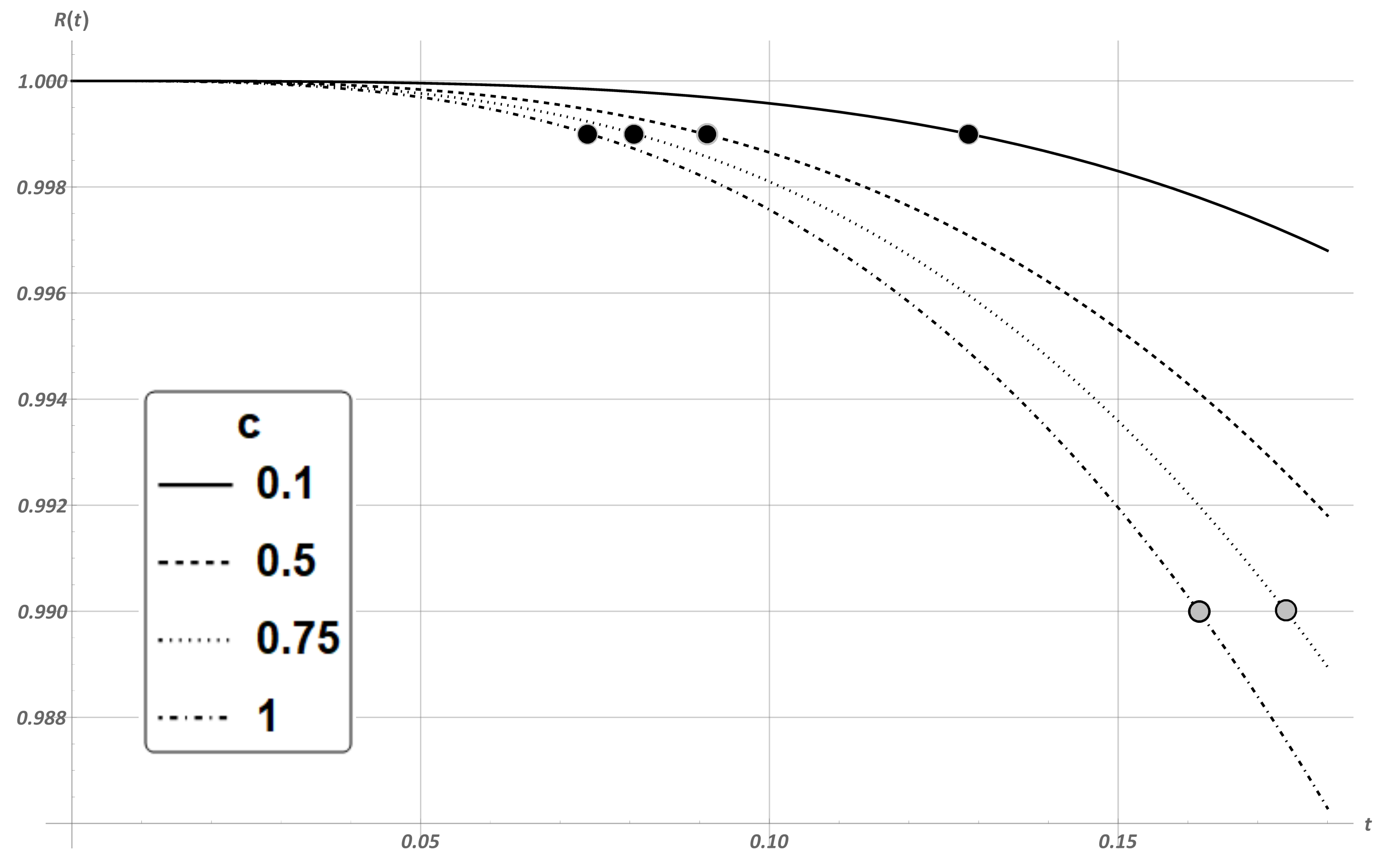
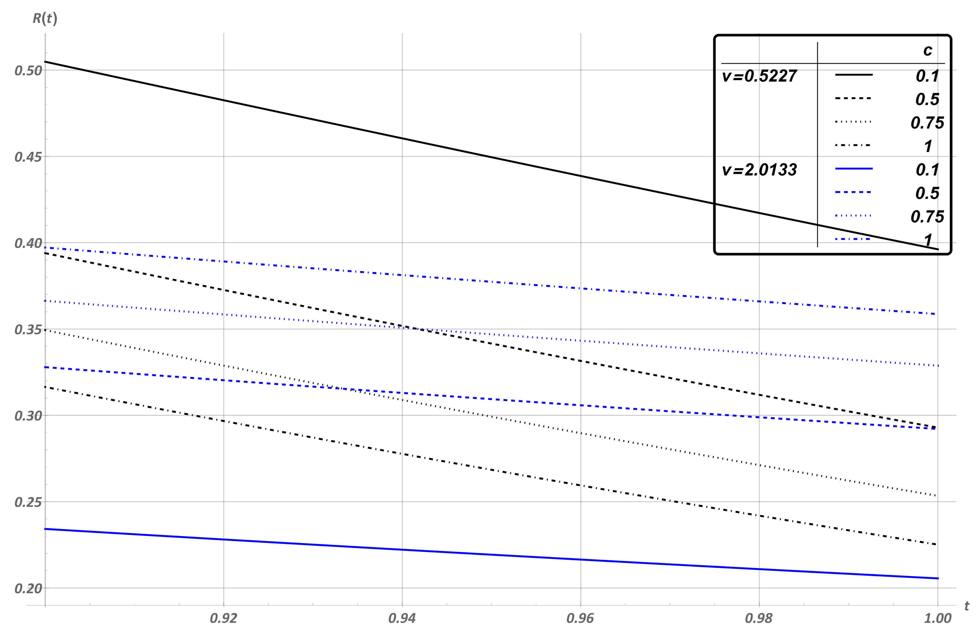
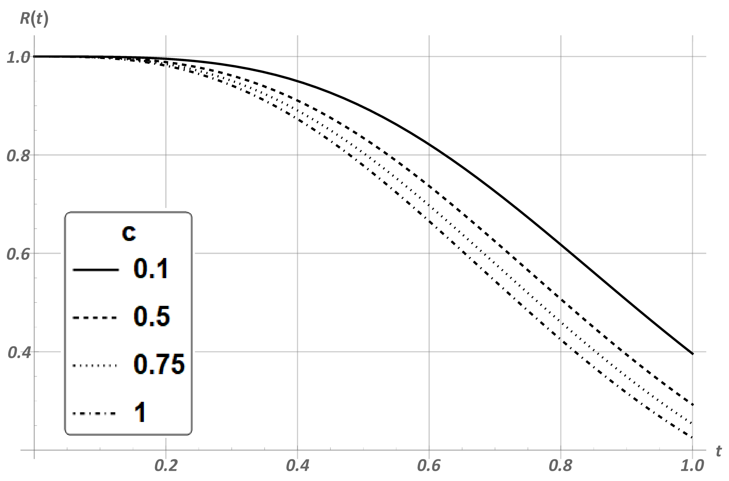
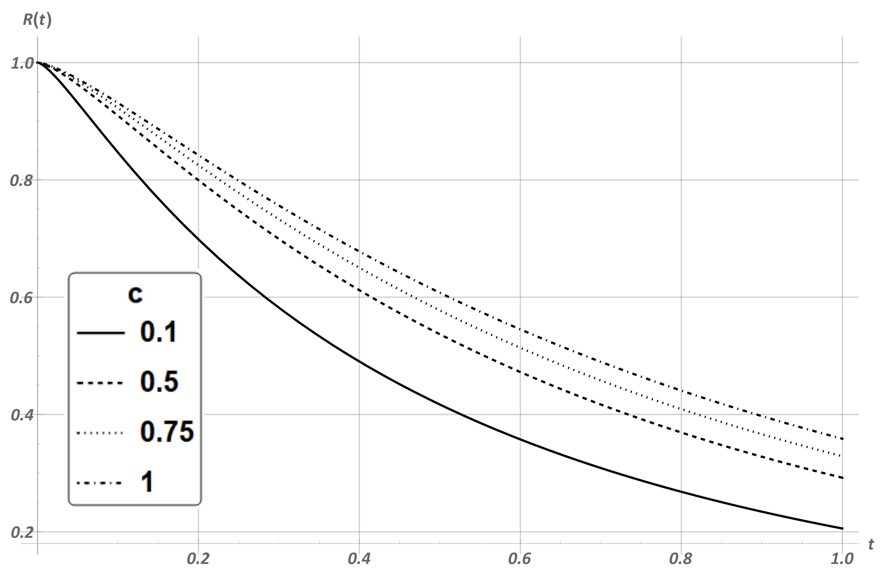
4. Numerical Experiment

As is known, the exponential distribution has no memory. Thus, the example in Section 3.3 does not show the effect of the load redistribution on surviving components after a failure. Thus, consider the Gnedenko–Weibull (GW) distribution as the distribution of the system’s components’ lifetime, $A\left(t\right)\sim GW\left(\theta ,{\displaystyle \frac{a}{\mathrm{\Gamma }(1+{\theta }^{-1})}}\right)$. Here, a is the timeof the component’s failure, $\theta$ is the shape parameter of the GW distribution calculated based on the preset value of the coefficient of variation, and $v={\displaystyle \frac{\sigma }{a}}=a^{-1}·\sqrt{{\displaystyle \frac{\mathrm{\Gamma }(1+2·{\theta }^{-1})}{\mathrm{\Gamma }{(1+{\theta }^{-1})}^2}}-1}$, where $\sigma$ is the standard deviation.

The hazard rate function for the GW distribution has the following form:

$$\alpha \left(t\right)=\theta {\left(\frac{\mathrm{\Gamma }(1+{\theta }^{-1})}{a}\right)}^{\theta }{t}^{\theta -1}.$$

According to the Algorithm 1, calculate the reliability function of a 2-out-of-3 system with the GW distribution of its components’ lifetime and present the result graphically.

Suppose that the mean lifetime of the component $a=1$. If $\theta =1$, the GW distribution transforms into an exponential one with the mean timea and the coefficient of variation $v=1$. In this case, its reliability function has the form of (10). Therefore, cases $0<v<1$ and $v>1$ are of interest. Since calculating the coefficient $\theta$ through the value v is quite difficult, we define the parameter $\theta$ so that $v\approx 0.5$ and $v\approx 2$. Thereby, define $\theta =2$, then the coefficient of variation $v=0.5227$. Assume that the aging time of the surviving components after failure is some percentage of the average lifetime of the components, $c_1=0.1;0.5;0.75;1$ from a.

Since the 2-out-of-3 system fails due to the failure of two components, we have only one constant that defines the aging time of surviving components. Therefore, hereafter, we suppose $c_1=c$. Figure 1 presents the reliability function of the 2-out-of-3 system with different c. According to this figure, the higher reliability coincides with the lower value of c.

Other reliability characteristics of the 2-out-of-3 system calculated according to the definitions from the algorithm are presented in

Table 1. System reliability characteristics.

	$\mathit{c}=0.1$	$\mathit{c}=0.5$	$\mathit{c}=0.75$	$\mathit{c}=1$
$\mathbf{E}\left[S_2\right]$	$0.9309$	$0.8324$	$0.7932$	$0.7639$
$\mathbf{Var}\left[S_2\right]$	$0.1238$	$0.1130$	$0.1081$	$0.1045$
$v\left[S_2\right]$	$0.3780$	$0.4038$	$0.4145$	$0.4231$

. These characteristics correspond to the system reliability behavior shown in Figure 1. The lower value of c leads to the higher value of the system lifetime expectation $\mathbf{E}\left[S_2\right]$. Moreover, with an increase in c, the coefficient of variation of the system $v\left[S_2\right]$ grows and tends to the value of the coefficient of variation of each system element $v\approx 0.5$.

To study the reliability of a system, a characteristic such as a quantile is often used. This measure shows how long the system will be reliable with a fixed probability. The quantiles $q_{\gamma }=R^{-1}\left(\gamma \right)$ of the reliability function are presented in Figure 2. In this case, black bottoms correspond to $\gamma =0.999$, whereas gray bottoms correspond to $\gamma =0.99$.

All the values for quantiles $\gamma =0.999;0.99;0.9$ are presented in

Table 2. Quantiles of reliability function.

	$\mathit{c}=0.1$	$\mathit{c}=0.5$	$\mathit{c}=0.75$	$\mathit{c}=1$
$q_{0.999}$	$0.13$	$0.09$	$0.08$	$0.074$
$q_{0.99}$	$0.249$	$0.192$	$0.174$	$0.16$
$q_{0.9}$	$0.495$	$0.415$	$0.386$	$0.364$

.

It can be seen from Table 1 and Table 2 that the system reliability $\ge 0.9$ for all considered values c is achieved with $q_{\gamma }\approx \frac{1}{2}·\mathbf{E}\left[S_2\right]$. That is, the system is in an operational state for about half of its average lifetime with a probability $0.9$. For more details, see

Table 3. The ratio of $\mathbf{E}\left[S_2\right]/q_{\gamma }$.

	$\mathit{c}=0.1$	$\mathit{c}=0.5$	$\mathit{c}=0.75$	$\mathit{c}=1$
$\mathbf{E}\left[S_2\right]/q_{0.999}$	$7.16$	$9.25$	$9.92$	$10.32$
$\mathbf{E}\left[S_2\right]/q_{0.99}$	$3.74$	$4.34$	$4.56$	$4.77$
$\mathbf{E}\left[S_2\right]/q_{0.9}$	$1.88$	$2.01$	$2.05$	$2.09$

. The ratio of the mean system lifetime to the quantile $q_{0.99}$ by averaging from c is $\mathbf{E}\left[S_2\right]/q_{0.99}\approx 4.35$, and for $q_{0.999}$, it holds $\mathbf{E}\left[S_2\right]/q_{0.999}\approx 9.16$.

It is known that for the GW distribution, the behavior of its hazard rate function depends on the shape parameter $\theta$, which affects the coefficient of variation. For the GW distribution, the value of the coefficient of variation $v>1$ leads to the value of parameter $\theta <1$. This leads to a decrease in the hazard rate function. Thus, the distribution becomes “rejuvenating”. Since this situation does not correspond to practical problems, we consider the case $v>1$ only as a curious example. Consider $\theta =0.54$. The coefficient of variation in this case is $v=2.0133$. With the same values c, the graph of the reliability function is presented in Figure 3. According to the graph, the relationship between reliability and c is inverse to the previous case. The higher reliability coincides with the higher value c.

Despite the different behavior of the curves in Figure 1 and Figure 3 in the vicinity of the point $t=1$, the reliability of the system for different values v converges to a small interval (Figure 4). The black lines correspond to $v=0.5227$, and the blue ones are for $v=2.0133$. The figure shows that for $t=1$ with $c=0.5$, the reliability function takes the same value with different v. The difference between the values of $R\left(1\right)$ with $c=0.75,1$ increases as c increases, but with the lower value $c=0.1$, the difference between $R\left(1\right)$ is greatest.

5. Conclusions

In this paper, a k-out-of-n system was considered in which the failure of any of its components leads to increasing the load on all others, which leads to a decrease in their residual lifetimes. The components and the whole system reliability are modeled in terms of their hazard rate functions. After any component failure, all surviving components “age” for some time $c_i$ depending on the number of the remaining components.

The method and the algorithm for the system reliability function and its two moments were proposed. The obtained results were verified in the case of an exponential distribution for the system components’ lifetime, in which an analytical solution was obtained with the usual finite state Markov process. Some numerical experiments with Gnedenko–Weibull system components were proposed.

A more detailed analysis of the sensitivity problems and some real applications of the model will be presented in the future.

References

1. Shepherd, D.K. k-out-of-n Systems. In Wiley StatsRef: Statistics Reference Online; Balakrishnan, N., Colton, T., Everitt, B., Piegorsch, W., Ruggeri, F., Teugels, J.L., Eds.; John Wiley & Sons: New York, NY, USA, 2014. [Google Scholar] [CrossRef]
2. Trivedi, K.S. Probability and Statistics with Reliability, Queuing and Computer Science Applications, 2nd ed.; John Wiley & Sons: New York, NY, USA, 2016. [Google Scholar]
3. Kuo, W.; Zuo, M.J. Optimal Reliability Modeling: Principles and Applications; John Wiley & Sons: New York, NY, USA, 2003. [Google Scholar]
4. Eryilmaz, S. Review of recent advances in reliability of consecutive k-out-of-n and related systems. Proc. Inst. Mech. Eng. Part O J. Risk Reliab. 2010, 224, 225–237. [Google Scholar] [CrossRef]
5. Levitin, G.; Xing, L.; Dai, Y. Heterogeneous 1-out-of-N warm standby systems with dynamic uneven backups. IEEE Trans. Reliab. 2015, 64, 1325–1339. [Google Scholar] [CrossRef]
6. Gertsbakh, I.; Shpungin, Y. Reliability Of Heterogeneous ((k, r)-out-of-(n, m)) System. RTA 2016, 11, 8–10. [Google Scholar]
7. Ushakov, I. A universal generating function. Sov. J. Comput. Syst. Sci. 1986, 24, 37–49. [Google Scholar]
8. Ushakov, I. Optimal standby problem and a universal generating function. Sov. J. Comput. Syst. Sci. 1987, 25, 61–73. [Google Scholar]
9. Levitin, G. The Universal Generating Function in Reliability ANALYSIS and Optimization; Springer Series in Reliability Engineering; Springer: London, UK, 2005. [Google Scholar]
10. Vishnevsky, V.M.; Kozyrev, D.V.; Rykov, V.V.; Nguyen, D.P. Reliability modeling of an unmanned high-altitude mobile of a tethered telecommunication platform. Inf. Technol. Comput. Syst. 2020, 4, 26–36. [Google Scholar] [CrossRef]
11. Cramer, E.; Kamps, U. Sequential order statistics and k-out-of-n systems with sequentially adjusted failure rates. Ann. Inst. Stat. Math. 1996, 48, 535–549. [Google Scholar] [CrossRef]
12. Liang, X.; Xiong, Y.; Li, Z. Exact Reliability Formula for Consecutive-k-Out-of-n Repairable Systems. IEEE Trans. Reliab. 2010, 59, 313–318. [Google Scholar] [CrossRef]
13. Gökdere, G.; Ng, H.K.T. Time-dependent reliability analysis for repairable consecutive-k-out-of-n:F system. Stat. Theory Relat. Fields 2022, 6, 139–147. [Google Scholar] [CrossRef]
14. Wu, Y.; Guan, J. Repairable consecutive-k-out-of-n: G systems with r repairmen. IEEE Trans. Reliab. 2005, 54, 328–337. [Google Scholar] [CrossRef]
15. Krishnamoorthy, A.; Rekha, A. k-out-of-n-System with Repair: T–Policy. Korean J. Comput. Appl. Math. 2001, 8, 199–212. [Google Scholar] [CrossRef]
16. Liu, H. Reliability of a load-sharing k-out-of-n:G system: Non-iid components with arbitrary distributions. IEEE Trans. Reliab. 1998, 47, 279–284. [Google Scholar] [CrossRef]
17. Sutar, S.; Naik-Nimbalkar, U.V. A load share model for non-identical components of a k-out-of-m system. Appl. Math. Model. 2019, 72, 486–498. [Google Scholar] [CrossRef]
18. Hellmich, M. Semi-Markov embeddable reliability structures and applications to load-sharing k-out-of-n system. Int. J. Rel. Qual. Safety Eng. 2013, 20, 1350007. [Google Scholar] [CrossRef]
19. Rykov, V.; Kochueva, O.; Farkhadov, M. Preventive Maintenance of a k-out-of-n System with Applications in Subsea Pipeline Monitoring. J. Mar. Sci. Eng. 2021, 9, 85. [Google Scholar] [CrossRef]
20. Rykov, V.; Kochueva, O.; Rykov, Y. Preventive Maintenance of k-out-of-n System with respect to Cost-type Criterion. Mathematics 2021, 9, 2798. [Google Scholar] [CrossRef]
21. Rykov, V.; Zaripova, E.; Ivanova, N.; Shorgin, S. On Sensitivity Analysis of Steady State Probabilities of Double Redundant Renewable System with Marshal-Olkin Failure Model. InDistributed Computer and Communication Networks; Vishnevskiy, V.V., Kozyrev, D.V., Eds.; Springer: Berlin/Heidelberg, Germany, 2018; pp. 234–245. [Google Scholar]
22. Rykov, V.; Ivanova, N.; Kozyrev, D. Sensitivity Analysis of a k-out-of-n:F System Characteristics to Shapes of Input Distribution. Lect. Notes Comput. Sci. (LNCS) 2020, 12563, 485–496. [Google Scholar] [CrossRef]
Figure 1. Reliability function with GW distribution of the components’ lifetime with v = 0.5227 .
Mathematics 10 02457 g001
Figure 2. Reliability function with v = 0.5227 and quantiles.
Mathematics 10 02457 g002
Figure 3. Reliability function with GW distribution of the components’ lifetime with v = 2.01325 .
Mathematics 10 02457 g003
Figure 4. Reliability function on t = 0.9 , 1 ¯ .
Mathematics 10 02457 g004