Abstract
Optimal control problems are applied to a variety of dynamical systems with a random law of motion. In this paper we show that the random degradation processes defined on a discrete set of intermediate degradation states are also suitable for formulating and solving optimization problems and finding an appropriate optimal control policy. Two degradation models are considered in this paper: with random time to an instantaneous failure and with random time to a preventive maintenance. In both cases, a threshold-based control policy with two thresholds levels defining the signal state, after which an instantaneous failure or preventive maintenance can occur after a random time, and a maximum number of intermediate degradation states is applied. The optimal control problem is mainly solved in a steady-state regime. The main loss functional is formulated as the average cost per unit of time for a given cost structure. The Markov degradation models are used for numerical calculations of the optimal threshold policy and reliability function of the studied degrading units.
Keywords:
degradation process; optimal control problem; threshold-based policy; average cost; Markov death process; reliability function MSC:
60K20; 90B25; 65C40
1. Introduction
In recent decades, due to the rapid development of sensor technologies, data transmission technologies, and monitoring systems, the tasks of controlling the aging and degradation of technical and biological objects have received additional impetus for research. Some wearing and aging models were in the focus of many investigators in the framework of shock and damage models. An excellent review and contribution of the earlier papers devoted to the topic can be found in the studies by Esary et al. [1], Kopnov and Timashev [2], and the references therein. Murphy and Iskandar [3] have studied the application of a control policy with two parameters to the degradation process associated with shocks. In Singpurwalla [4], the hazard potential notion as a random life resource has been introduced and considered. Then, this notion was investigated in different directions in Singpurwalla [5]. The aging and degradation models suppose the study of systems with gradual failures for which multi-state reliability models were elaborated (for the history and bibliography see, e.g., Lisniansky and Levitin [6]). Rykov and Dimitrov [7] proposed the model for complex hierarchical reliability system. Rykov and Efrosinin [8] studied the controllable degradation unit as the fault tolerance unit. Generalized birth and death processes as degradation models were considered in Rykov [9]. A degrading unit with random life resources, which operates until complete failure occurs, was analyzed by Rykov and Efrosinin [10]. Giorgio et al. [11] proposed a Markov model for the gradual deterioration process, which progressively degrades until a complete failure occurs. The regenerative variant of the splitting method to estimate the failure probability in a controllable degradation process was provided in Borodina et al. [12].
Let the mechanical or biological system contain a degrading unit. Degradation processes under study are assumed to have observable states or there is some observable measure parameter that can be associated with a process, e.g., signal of acoustic emission, ultrasonic method for the detection of hidden defects, measures of the gravimetric analysis, and electromagnetic flaw detection. The degradation process is broken down into discrete stages, the dwell times of which are random. Two types of systems are of special interest. In first case the degrading unit has a random time to an instantaneous failure while in the second case the degrading unit has a random time to a preventive repair. In both cases the unit is of multiple uses, i.e., after a complete failure it can be repaired. After the repair, the degradation process starts again in an absolutely new state. The unit is supplied by a monitoring system and by a controller. The monitoring system gives the information about the current degradation state and, based on this information, the controller makes a decision about a necessity to perform the preventive repair until the last degradation state is achieved. The control problem is studied in a stationary regime. The control principles of such degradation systems may be easily explained by virtue of the following examples. Some of them were introduced in Kopnov [13].
Corrosion process of a unit with protective covering. Let a unit subjected to corrosion have a protective covering, which decreases during operation, and make it possible to trace its thickness, see Figure 1. The problem is to find the optimal value of the initial thickness and the thickness when the covering should be renewed.
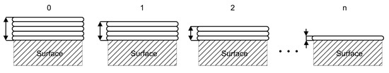
Figure 1.
Corrosion process.
Damage process due to the fatigue crack growth. Let a unit fail due to the fatigue crack growth, as illustrated in Figure 2. The unit can be supplied by a fatigue gauge that can be e.g., as a plane notched pattern. This gauge works with the unit and reflects its damage accumulation process. The problem is to find the optimal value of the gauge’s crack when stopping and replacement are implemented. The recovery of of such a unit can be also performed by means of the welding.
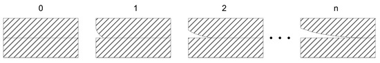
Figure 2.
Fatigue crack growth.
Wear of the tool of machine-tools. The wear of the machine tools is correlated with thermo-emf of the pair “cutter-blank”. A monitoring system can be installed, and the optimal value of the measured voltage can be determined to prevent failures and outputs of poor quality.
Wear of a plane bearing. The bearing is a critical unit of a piece of metallurgical equipment, hence the optimal maintenance problem of a plain bearing must be discussed. The restoration cost of the failed system is higher than the inspection and preventive replacement cost. In Ref. [14], the authors investigate the bearing shell wear process as a degradation one.
Discharge of an external load. If the degradation process is associated with external loads, and a unit fails when the load exceeds a failure level, then partial or full discharge of loads is another example of the controllable damage process.
In this paper we consider degradation systems operating under a threshold-based policy with threshold levels . Here, the first threshold level m specifies a state, where a controller receives a signal that after a random time for one type of degenerating process an instantaneous failure may occur or for another type a preventive repair may take place. The second threshold n stands for the maximal number of gradual failure states before hitting a complete failure state. In corrosion processes the pair defines the appropriate thickness of the protective covering and the thickness where a signal should be generated. In a damage process the pair defines the maximal size of the crack and the corresponding signal size. The proposed approach for optimization of the degradation process has a number of advantages. The optimal control policy depends on only two parameters, which can be calculated relatively easily. The performance and reliability characteristics of the degraded units are obtained explicitly. Assuming that the input random variables belong to parametric families of distributions, then, in practice, for a degradation process with discrete phases, the unknown parameters of the distributions can be easily estimated from statistical data.
The paper is organized as follows. In Section 2, we describe the mathematical model of the degrading unit with a random time to an instantaneous failure and derive the performance and reliability characteristics. In Section 3, we develop the analysis for the mean losses and reliability function for the model of the degrading unit with random time to a preventive repair. Some illustrative numerical examples are discussed in Section 4.
In order to make it easier to understand the description of the mathematical models and the corresponding results, we have summarized the main notations together with their descriptions in Table 1.

Table 1.
List of the main notations used in the paper.
2. Degrading Unit with an Instantaneous Failure
2.1. Mathematical Model
Consider a degradation process with a discrete set of states , where n stands for the maximal possible number of intermediate degradation states up to a complete failure state F. Until a degradation state m with , which is referred to as a signal state, is reached, only a gradual deterioration of the unit can take place. After reaching state m both another gradual failure and an instantaneous failure can occur, leading the deteriorating unit to a complete failure state F. The diagram of possible realization of the process is illustrated in Figure 3.
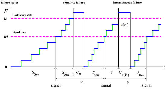
Figure 3.
Realization of a degrading process under threshold policy .
The following notations are used in the figure: —time to reach state from state , where is a random variable of a sojourn time in state , V is a random time to an instantaneous failure after entering the state m, is a random repair time after a failure in state . After the degradation process has reached the signal state m, two events are possible, according to a specified model. Either instantaneous failure occurs after a random time V, or there is a transition to the last degradation phase and a subsequent failure in time . After an instantaneous failure, the unit is restored in a random period of time , where is a current gradual degradation state at the moment of the instantaneous failure. After restoration, the unit becomes as good as new, i.e., the degradation process starts again from state 0. For distribution functions of introduced random variables, we use the following notations:
As a recovery control we consider a two-level control policy to repair the system given that the signal state is m with a total number of degradation states n. We further introduce an additional cost structure associated with the functioning of the deteriorating unit: —a repair cost per unit of time after a complete failure in state , —a fixed cost due to a complete failure after passing all degradation states, —a fixed cost due to an instantaneous failure, —operational cost per unit of time in state .
2.2. Regenerative Process with Costs
The degradation process can be represented in the form of a regenerative process whose regenerative moments are the moments of visiting the signal state m, as shown in Figure 3. Denote by the average duration of a regenerative cycle, and by the average cost in this cycle for the policy . We distinguish between two types of regenerative cycles, where the random variables and can be represented in the following way,
where is a random holding time in state i in a regenerative cycle.
Proposition 1.
The average duration of a regenerative cycle for the threshold policy is derived from a relation
where is the probability of an instantaneous failure in one regenerative cycle.
Proof.
Proposition 2.
The average cost per unit of time in a regenerative cycle is derived from a relation
Proof.
The relation (4) follows directly from the definition (2) and the law of the total probability. □
From the theory of regenerative process it is known that the average cost per unit of time under the control policy can be expressed as
where the failure probability and expectations can be calculated by
In addition to the average cost per unit of time, an analysis of the degradation process can include a calculation of the average time to the first failure of the unit given that the initial state is ,
the steady-state probability of the failure state F,
and the availability of the unit ,
2.3. Markov Degradation Model
In a special case of random variables with exponential distributions, , , , and , we explicitly get the expectations
To derive the expressions for and other expectations in (6), consider an auxiliary death process describing a continuous-time Markov chain with a set of states and an absorption in state F. Denote by the transition probability of the death process at time t given that the initial condition is and for , . The probability can be derived from the system of Kolmogorov’s differential equations. Applying the Laplace transform to this system and following [15], we obtain the following statement.
Proposition 3.
The probabilities satisfy the system of differential equations
which has the unique solution
where , in particular
Corollary 1.
From Proposition 3 it follows that
Proof.
These expressions follow directly from (6) and the convolution property in the case of independent random variables. □
Denote by the reliability function of the degradation process.
Proposition 4.
The reliability function is of the form
where
Proof.
The life time T of the degradation unit is defined as and then, due to Proposition 3, we get
After substituting the distribution functions , and the probability density function into the last expression after some algebra, we get
Then, the subsequent integration leads to the expression (12). □
2.4. Numerical Examples
Let us consider a system with a maximal possible number of gradual degradation states , where a signal state . We assume the following monotonicity for the ordering of the values of system parameters, namely, , , , . Moreover let , , in this case we assume that the instantaneous failure is a quite rare event, comparing the transitions over the graduate degradation states. We allow the parameters of the degradation process to take the following values by taking the above-mentioned considerations into account: ,
Further we fix the costs at the following values:
Example 1.
This example presents the results of calculating the optimal threshold policy , which minimizes the average cost per unit of time defined in (5) as a function of different costs. One type of cost is set to be varied, while all other parameters take the fixed values as defined above.
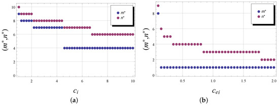
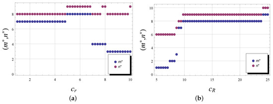
In Figure 4, we display the optimal policy as the repair cost (the figure labeled by “a”) and the operational cost (the figure labeled by “b”) per unit of time varies. The blue cycles tag the values for the optimal signal state , while the magenta cycles tag the optimal values for the number of gradual failures . For example, if , the optimal policy is equal to , and if , then . If , then , and if , then . As can be seen from the figure, both thresholds are quite sensitive to an increase in the repair cost, and both thresholds are decreasing monotonously. At the same time, an increase in the operating costs also leads to a decrease in the signal threshold, but the total number of degradation phases has little sensitivity to an increase in this type of costs. The influence of the fixed costs and is shown in Figure 5 (the figure labeled respectively by “a” and “b”). The figure illustrates, that, e.g., for , the optimal policy , and for , .
Figure 4.
versus (a) and (b) for the model with an instantaneous failure.
Figure 5.
versus (a) and (b) for the model with an instantaneous failure.
We observe here non-monotonic changes in thresholds as the cost after a complete failure increases. For example, for , the optimal policy , for , , and for , we get . In the figure, where the fixed cost due to an instantaneous failure increases, the optimal thresholds increases again monotonously. For example, if , the , and, if , the .
Example 2.
In this example we compare the different optimization problems specified in (10). In Table 2, we evaluate the optimal thresholds for different optimization problems given that the signal threshold takes a fixed value . The parameters of the deteriorating unit take on the values given at the beginning of the section.
Table 2.
Comparison of different optimization problems for the model with an instantaneous failure.
As can be seen from these calculations, depending on the optimizing function, the solution for the optimal threshold policy differs considerably. Thus, when formulating the optimization problem, it is also necessary to pay close attention to the possible constraints on the values of other quantitative characteristics of the degrading unit.
Example 3.
In this example we analyze the effect of the optimal policy evaluated with respect to optimization problems; see Cases 1–5 enumerated in Table 2, and the intensity of the instantaneous failure ν on the reliability function in (12).
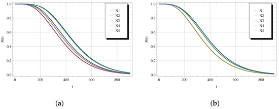
In Figure 6, the intensity (the figure labeled by “a”) and (the figure labeled by “b”). We report the numerical examples to show the reliability function for the optimal threshold policies . We can point out that for , Cases 5 and 2 correspond respectively to the boundary cases of the most and less reliable degrading unit. The curves of other cases are located between these boundaries, which coincides with the results from Table 2. If increases, we observe that in all cases the unit becomes less reliable, moreover, the curves for Cases 2, 3, and 5 coincide. In this figure, the most reliable model corresponds to Case 1. This result does not contradict the fact that the model in Case 5 maximizes the mean time to failure, since the signal threshold m is fixed in the calculation data and optimization is only based on the value of the second threshold n.
Figure 6.
for (a) and (b).
3. Degrading Unit with a Partial Preventive Repair
In this section we consider a deteriorating unit that degrades according to a degradation process , whose trajectory is illustrated in Figure 7.
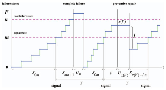
Figure 7.
Realization of a degrading process under threshold policy with .
The notations associated with this model are the same as previously. According to this model, the degradation process has the set of space as before. After reaching the signal state m, two events are possible: either there is a partial preventive repair in a random time V, which occurs in a degradation state with a state-dependent repair time , or in time , where there is a transition to a complete failure state and where the unit can be completely recovered in a random time . After a preventive repair in state , we assume that the unit may not be so good as a new one, and it returns to the gradual failure state , where .
3.1. Regenerative Process with Costs
The proposed degradation process can be treated again as a regenerative one, where the hitting times of the signal state m are the regenerative moments. In a similar was as before, we distinguish between two types of cycles with and without a complete failure within it. The random variables and are then of the form,
Let us denote by the probability of a complete failure in a regenerative cycle. Then, the following statement holds.
Proposition 5.
The average duration and average cost in a regenerative cycle satisfies the relations
where
and
Proof.
The proof of this statement is based on relations (13) and (14), and it is similar to that applied to the first model with instantaneous failures. The details are omitted here. □
3.2. Mean Time to Failure
As there are preventative repairs in this model, the random time T to complete failure will consist of other components. Let us introduce the following notations: —the random time from the beginning of the regenerative cycle until the moment of a complete failure if it occurs, —the random duration of the regenerative cycle without a complete failure, and N—the random number of cycles to complete failure. Since the complete failure occurs in each regenerative cycle with the probability , the number of cycles N has a geometric distribution, i.e.,
Then the mean time to the first complete failure is of the form.
Proposition 6.
The mean time to the first complete failure given that the initial state is satisfies the relation,
Proof.
Due to the structure of the random variable T and the law of the total probability, we have,
Consistent with the definition introduced for random variables and , we obtain and . By substituting these expectations into the last expressions and subsequent taking into account that after some simple algebra, we get the relation (15). □
Now we will briefly discuss the problem of calculating the reliability function . Let us assume that the complete failure of the system is a rare event. Further, we introduce the following notation: —the random time from the beginning of the regenerative cycle up to the time moment of the first complete failure within the Nth cycle. Due to the limiting theorem for the sojourn time of ergodic regenerative processes (see, e.g., [16]) the following statement holds.
Proposition 7.
Let the failure in one regenerative cycle be a rare event, i.e., the number of regeneration cycles N is significantly large. If for some , then for each the following asymptotic property can be derived,
where
In assumption of the Markov property, the reliability function of the degradation unit with an arbitrary can be calculated explicitly. The calculation is performed by means of conditional Laplace transforms , , of the probability density function for the residual life time given that the initial state is i. Obviously, in absorbing state F the conditional Laplace transform .
Proposition 8.
The Laplace transform of the reliability Function satisfies the relation,
where
Proof.
The time T is a duration commencing the initial state of the degradation process 0 and ends when the degrading unit visits the complete failure state F. The first-step analysis is employed for the Markov chain with an absorption in state F to get the system of equations for the conditional Laplace transforms , .
In (18), the equality for state i includes the term at , which represents the transition with a rate to a preventive maintenance state, from which the unit moves to a newer gradual failure state after an exponentially distributed time with a parameter . Solving recursively equations (18) and using for convenience the notations , and from the statement, we obtain explicit solutions for this system. In particular for the function after some simple algebra we have
The statement further follows from the fact that the Laplace transform and the conditional Laplace transform satisfy the relation
□
The inverse transformation of the function is required to get . Differentiation of the function with respect to the parameter s at point results in the mean life time to a complete failure, i.e.,
3.3. Numerical Examples
We next present the numerical examples involving the optimal policy for different optimization problems and the numerical inversion of the transform . In the following examples we assume that , , and . Moreover, , , , , where , and the costs , , and take the same values as for the previous model. We further fix .
Example 4.
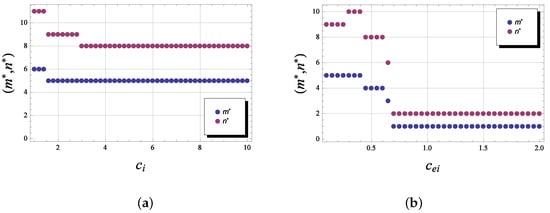
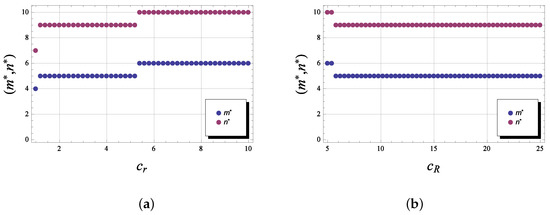
In Figure 8, we calculate the optimal policy as the cost (the figure labeled by “a”) and the cost (the figure labeled by “b”) varies. For example, the figure for the repair cost shows that if , then the optimal policy is , and if , then we obtain . From the figure for the operating cost , we can see that if , then the optimal policy is respectively equal to . Thus, the values of the optimal thresholds decrease monotonically with an increase in the cost , while we no longer observe such monotonicity with an increase in the cost . Moreover, at high operating costs, it becomes advantageous to limit the number of intermediate degradation states to a small number, i.e., by the policy , so that the unit can be repaired to an almost new state after a complete failure.
Figure 8.
versus (a) and (b) for the model with a preventive repair.
The influence of the repair costs and is illustrated in Figure 9 (the figure labeled respectively by “a” and “b”). Here we observe, for example, that if , the policies are optimal, and if , we then get the optimal policies . In both cases the changes are monotonic, although the optimal control appears to be less sensitive to an increase in the cost .
Figure 9.
versus (a) and (b) for the model with a preventive repair.
Example 5.
Table 3 summarizes the results of the calculations of optimal threshold levels for the different optimization criteria proposed in (10). In this case, just as in the previous degradation model, we obtained completely different optimal thresholds for different optimization criteria. The highest mean time to failure is naturally given by optimizing the function , i.e., . However, we obtained the shortest mean time to failure by minimizing the steady-state probability of a complete failure state , i.e., , which is not an obvious result.
Table 3.
Comparison of different optimization problems for the model with a preventive repair.
Example 6.
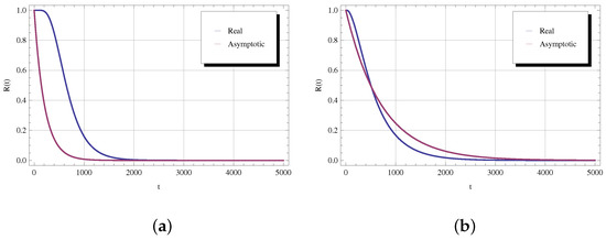
In Figure 10, we take (the figure labeled by “a”) and (the figure labeled by “b”). The control policy in both cases is . The other parameters take on the values defined above and display the real reliability function as a numerical inversion of the Laplace transform from (17), together with the asymptotic function (16). The asymptotic function is defined respectively by with , , and with , .
Figure 10.
Real and asymptotic reliability functions for (a) and (b).
We observe here that in the figure, which corresponds to a lower value for the probability of complete failure in a regeneration cycle , the asymptotic curve better approximates the corresponding real reliability function.
4. Conclusions
We investigated two types of degradation processes on a set of intermediate degradation states with the random time to an instantaneous failure and the random time to a preventive repair. In both cases, the rationality of using a two-threshold control policy to optimize a range of performance and reliability characteristics of degraded systems was confirmed. Thus, when modeling and putting into operation the technical units subject to a progressive process of degradation, it is possible to use the results of this work to provide the monitoring system with information about the optimal signal state and the optimal maximum number of discrete intermediate degradation states. In the case of the death Markov process, the reliability characteristics of the presented degradation units can be calculated analytically.
Author Contributions
Conceptualization, D.E.; Formal analysis, D.E. and N.S.; Methodology, D.E.; Software, N.S.; Writing—review & editing, D.E. All authors have read and agreed to the published version of the manuscript.
Funding
Open Access Funding by the University of Linz. This paper has been supported by the RUDN University Strategic Academic Leadership Program (recipient D. Efrosinin).
Data Availability Statement
Not applicable.
Acknowledgments
The authors acknowledge the financial support by the Johannes Kepler University Linz. This paper has been supported by the RUDN University Strategic Academic Leadership Program (recipient D. Efrosinin).
Conflicts of Interest
The authors declare no conflict of interest.
References
- Esary, J.D.; Marshall, A.W.; Proshan, F. Shock models and wear processes. Ann. Probab. 1973, 1, 627–649. [Google Scholar] [CrossRef]
- Kopnov, V.A.; Timashev, S.A. Optimal death process control in two-level policies. In Proceedings of the 4th Vilnius Conference on Probability Theory and Statistics, Vilnius, Lithuania, 24–29 June 1985; Volume 4, pp. 308–309. [Google Scholar]
- Murphy, D.N.P.; Iskandar, B.P. A new shock damage model: Part II—Optimal maintenance policies. Reliab. Eng. Syst. Saf. 1991, 31, 211–231. [Google Scholar] [CrossRef]
- Singpurwalla, N.D. The hazard potential: Introduction and overview. J. Am. Stat. Assoc. 2006, 101, 1705–1717. [Google Scholar] [CrossRef]
- Singpurwalla, N.D. Reliability and Risk; Wiley & Sons Ltd.: Chichester, UK, 2006. [Google Scholar]
- Lisnuansky, A.; Levitin, G. Multi-State System Reliability. Assessment, Optimization and Application; World Scientific: Hackensack, NJ, USA; London, UK; Singapore; Hong Kong, China, 2003. [Google Scholar]
- Rykov, V.; Dimitrov, B. On multi-state reliability systems. In Proceedings of the Seminar Applied Stochastic Models and Information Processes, Barcelona, Spain, 8–13 September 2002; pp. 128–135. [Google Scholar]
- Efrosinin, D.; Rykov, V. On reliability control of Fault Tolerance Units. In Proceedings of the Forth International Conference on Mathematical Methods in Reliability, Santa Fe, NM, USA, 21–25 June 2004. [Google Scholar]
- Rykov, V. Generalized birth and death processes and their application to aging models. Autom. Remote Control 2006, 3, 103–120. [Google Scholar]
- Rykov, V.; Efrosinin, D. Degradation models with random life resources. Commun. Stat. Theory Methods 2010, 39, 398–407. [Google Scholar] [CrossRef]
- Giorgio, M.; Guida, M.; Pulcini, G. An age- and state-dependent Markov model for degradation processes. IIE Trans. 2011, 43, 621–632. [Google Scholar]
- Borodina, A.; Efrosinin, D.; Morozov, E. Application of Splitting to Failure Estimation in Controllable Degradation System. In DCCN 2017: Distributed Computer and Communication Networks; Communications in Computer and Information Science; Vishnevskiy, V., Samouylov, K., Kozyrev, D., Eds.; Springer: Cham, Switzerland, 2017; Volume 700. [Google Scholar]
- Kopnov, V.A. Optimal degradation process control by two-level policies. Reliab. Eng. Syst. Saf. 1999, 66, 1–11. [Google Scholar] [CrossRef]
- Kopnov, V.A.; Kanajev, E.I. Optimal control limit for degradation process of a unit modeled as a Markov chain. Reliab. Eng. Syst. Saf. 1994, 43, 29–35. [Google Scholar] [CrossRef]
- Gnedenko, B.V. The Questions of the Mathematical Theory of Reliability; Radio and Communications: Moscow, Russia, 1983. (In Russian) [Google Scholar]
- Solovyev, A.D. Asymptotic behaviour of the time to the first occurrence of a rare event. Eng. Cybern. 1971, 9, 1038–1048. [Google Scholar]
Publisher’s Note: MDPI stays neutral with regard to jurisdictional claims in published maps and institutional affiliations. |
© 2022 by the authors. Licensee MDPI, Basel, Switzerland. This article is an open access article distributed under the terms and conditions of the Creative Commons Attribution (CC BY) license (https://creativecommons.org/licenses/by/4.0/).