Abstract
Conventional liquids have poor thermal conductivity, thus limiting their use in engineering. Therefore, scientists and researchers have created nanofluids, which consist of nanoparticles dispersed in a base fluid, to improve heat transfer properties in various fields, such as electronics, medicine, and molten metals. In this study, we examine the micropolar nanofluid flow in a stagnation region of a stretching/shrinking sheet by employing the modified Buongiorno nanofluid model. The nanofluid consists of magnetite (Fe3O4) nanoparticles. The similarity equations are solved numerically using MATLAB software. The solution is unique for the shrinking strength . Two solutions are found for the limited range of when . The solutions terminate at in the shrinking region. The rise in micropolar parameter contributes to the increment in the skin friction coefficient and the couple stress , but the Nusselt number and the Sherwood number decrease. These physical quantities intensify with the rise in the magnetic parameter . Finally, we investigated the stability of the solutions over time. This work contributes to the dual solution and time stability analysis of the current problem. In addition, critical values of the main physical parameters are also presented. These critical values are usually known as the separation values from laminar to turbulent boundary layer flows. In this case, once the critical value is achieved, the process for the specific product can be planned according to the desired output to optimize the productivity.
MSC:
76D10
1. Introduction
Nanofluid is obtained by adding nano-sized particles to a base fluid, first inspired by Choi and Eastman [1]. The idea is to boost the thermal conductivity of the base fluid by utilizing the nanoparticles. This concept was improved further by adding two different types of nanoparticles to the base fluid. This new mixture was termed a ‘hybrid nanofluid’. Related works on nanofluids and hybrid nanofluids can be found in Refs. [2,3,4,5,6,7,8,9,10].
Most manufacturing processes compromise with fluids such as colloidal solutions, lubricants, biological fluids, paints, and polymeric suspensions, which are non-Newtonian. In this regard, Eringen [11,12] introduced the theory of micropolar fluids to explain the microscopic properties of these fluids. Then, many researchers considered micropolar fluids in their studies, with a variety of flow conditions, such as stagnation flow [13,14,15] and mixed convection flow [16,17,18,19,20,21,22]. The flow of micropolar nanofluids using the Buongiorno model of nanofluid [23] has been examined by several researchers [24,25,26,27,28,29,30]. Buongiorno [23] considered seven slip mechanisms that can produce a relative velocity between the nanoparticles and the base fluid. These are inertia, Brownian diffusion, thermophoresis, diffusiophoresis, the Magnus effect, fluid drainage, and gravity. They concluded that Brownian diffusion and thermophoresis are two important primary slip mechanisms between solid and liquid phases in nanofluids. Based on this finding, they developed a two-component, four-equation nonhomogeneous equilibrium model for mass, momentum, and heat transport in nanofluids. The effect of nanoparticles on micropolar fluid was reported in Refs. [31,32,33,34,35,36]. Refs. [37,38,39,40,41,42,43,44,45] are also relevant in this regard.
The combination of two nanofluid models, introduced by Tiwari and Das [3] and Buongiorno [23], has gained much attention from researchers. This model is called the modified Buongiorno model for nanofluid, where the Brownian motion and thermophoresis effects are taken into consideration. For example, Patel et al. [46] employed this model by considering the micropolar fluid. Several studies that also employed this model can be found in Refs. [47,48,49,50,51].
The stagnation point flow describes the motion of fluid near the stagnation region on a stationary or moving solid surface. Physically, a stagnation point refers to a point in the flow field where the local velocity is zero [52]. Analogously, stagnation point flow can be described as a jet of water impinging on a rigid body [53]. The static pressure of the fluid is maximum at the stagnation point and is known as the stagnation pressure, while the temperature at the stagnation point is known as the stagnation temperature [54]. In addition, the kinetic energy at the stagnation point is completely converted to internal energy since the fluid velocity is zero at that point. The region around the stagnation point receives the highest pressure, heat transport rate, and mass storage. Moreover, the existence of the stagnation flow velocity can confine the vorticity to maintain the flow in the shrinking sheet; thus, the application of suction is not necessary, as discussed by Wang [55]. Moreover, the phenomenon of the flow in a stagnation region commonly occurs in aerodynamic industries and engineering applications such as in polymer extrusion, drawing of plastic sheets, and wire drawing.
Magnetohydrodynamics, or MHD for short, is a study that involves a combination of the concepts of fluid dynamics and electromagnetism. A fluid flowing across a magnetic field will produce an electric current capable of influencing the flow behavior and also the temperature of the fluid. The theory of laminar flow of an electrically conductive fluid in a homogeneous magnetic field was pioneered by Hartmann [56]. Later, Pavlov [57] considered the boundary layer flow problem of an electrically conducting fluid in the presence of a uniform transverse magnetic field on a plane elastic surface. MHD flow of electrically conductive fluids is also important in modern metallurgical and metal working processes such as metal assembly processes in electric furnaces using magnetic fields and wall cooling processes in nuclear reactor containment chambers [58]. Furthermore, the MHD concept is also used in thermal power generation systems that are able to convert thermal energy into electrical energy [59].
The terms radiant heat transfer and thermal radiation are commonly used to describe heat transfer caused by electromagnetic waves [60]. Rosseland [61] is the researcher who introduced the thermal radiation model by using diffusion theory to study the effect of thermal radiation in astrophysics. For applications in certain spaces, some devices are designed to operate at high temperature levels to obtain maximum thermal efficiency. Thus, the effect of thermal radiation is important in determining the effect of heat in a process with high temperature. Therefore, thermal radiation makes a significant contribution to energy transfer processes in furnaces, combustion chambers, rocket plumes, high-temperature heat exchangers, and during chemical explosions [62].
The study of chemical reactions is of interest in bioengineering and chemical industrial applications, including food processing, polymer production, evaporation, ceramic manufacturing, drying, energy transport between cooling towers, and desert cooling streams. The influence of chemical reactions on heat and mass transfer on a stretchable rotating disk was reported by Muthtamilselvan et al. [63]. Moreover, Rawat et al. [64] studied the effect of chemical reaction on the flow over a cone and a wedge. Singh et al. [65] reported the numerical solution of micropolar fluid flow through a stretchable surface with chemical reaction and melting heat transfer. Xiong et al. [66] examined Reiner–Philippoff fluid with chemical reaction effects.
The present study considers the flow of a micropolar fluid past a shrinking sheet containing a magnetite nanoparticle (Fe3O4) by employing the modified Buongiorno nanofluid model. Different from Patel et al. [46], the present study investigates the flow behavior in the stagnation point region.
2. Mathematical Formulation
A steady laminar stagnation point flow on a stretching or shrinking sheet immersed in a micropolar fluid with Fe3O4 nanoparticles was evaluated (see Figure 1). The surface stretched or shrunk with velocity where is a constant, with for stretching and for shrinking. The external flow is represented by with . The transverse magnetic field is applied normally to the surface. A few assumptions are considered for the physical model. The hybrid nanofluid is assumed to be stable. Thus, the effect of nanoparticle aggregation and sedimentation is omitted. The nanoparticles are assumed to have a uniform size with a spherical shape. It is assumed that both the base fluid and nanoparticles are in a thermal equilibrium state, and they flow at the same velocity.
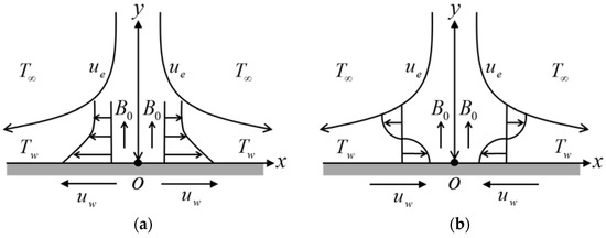
Figure 1.
The flow configuration of (a) stretching and (b) shrinking sheets.
Accordingly, the equations that govern the flow are [3,23,46]:
subject to:
where are the velocity components, is the vortex viscosity, is the microrotation velocity, is the micro-gyration parameter, is the Stefan–Boltzmann constant, is the mean absorption coefficient, and is the effective heat capacity ratio. and are the coefficients of the Brownian motion and the thermophoretic diffusion, respectively. is the first-order chemical reaction rate. and represent the temperature and the concentration, respectively. Here, the concentration at the surface and the temperature at the surface are assumed to be constant. Moreover, the spin gradient viscosity and the microinertia coefficient are defined as:
The thermophysical properties are given in Table 1 and Table 2, which are adapted from Refs. [4,46]. The nanoparticle volume fraction is represented by , while the subscript corresponds to its solid component. The subscript is for nanofluid and signifies the base fluid.

Table 1.
Thermophysical properties of Fe3O4 nanoparticle and water.
Table 2.
Thermophysical properties of nanofluid.
The following dimensionless variables are utilized [13,46]:
where is the stream function. We define and , then:
which satisfy the continuity Equation (1). Equations (2)–(5) are respectively transformed into:
subject to:
In the above equations, is the material parameter, is the magnetic parameter, is the Prandtl number, is the radiation parameter, is the Brownian motion parameter, is the thermophoresis parameter, is the Schmidt number, is the chemical reaction parameter, and is the stretching or shrinking parameter, defined as:
with is for shrinking, is for stretching, and is for the static sheet.
The quantities of physical interest are the skin friction coefficient , local couple stress , the local Nusselt number , and the local Sherwood number , which are expressed as [21,28]:
Using Equations (8) and (16), we obtain:
where the local Reynolds number is given as .
3. Stability Analysis
The stability of the dual solutions is determined by adapting the procedures introduced by Merkin [67] and Weidman et al. [68], considering the new variables as:
where is nondimensional time. Then, we obtain:
Substituting Equations (18) and (19) into the unsteady form of Equations (2)–(5) yields:
subject to:
The perturbations are introduced to the steady solutions , , , and of Equations (10)–(13) by employing the following relations [68]:
The signs of determine the stability of the solutions. It is noted that ,, , and are relatively small compared to , , , and . The perturbations (25) are applied and the eigenvalues are obtained by solving Equations (20)–(24). After linearization and by setting , then , , , and . The final form of the eigenvalue problems reads as follows:
subject to:
The values of in Equations (26)–(29) are obtained for the case (see Harris et al. [69]).
4. Results and Discussion
Equations (10)–(14) are numerically solved using the bvp4c package in the MATLAB software [70]. This solver occupies a finite difference method that employs the three-stage Lobatto IIIa formula with fourth-order accuracy. To achieve the accuracy of the numerical values, the selection of the initial guess and the boundary layer thickness, , must be precise. Moreover, the accuracy is also dependent on the values of the parameters applied for the computation. The results are presented for the physical quantities of interest given in Equation (17). Moreover, the velocity, concentration, and temperature profiles, as well as the stream function, are plotted to support the validity of the numerical results. The code is run for a set value of parameters. The validity of the outcomes is checked by examining the related profiles. Correct profiles must approach the infinity boundary conditions (14) asymptotically and not intersect with the horizontal axes (see Pantokratoras [71]). Moreover, the numerical outcomes are compared with the existing results available in the literature for a special case of the present study.
The values of when , , and for and are presented in Table 3, along with the results of Wang [55] and Ishak et al. [13], which show good agreement. Table 4 shows the effects of various parameters on when and . It can be seen that some parameters such as , , and have a significant impact on these quantities. This is because the similarity equations, i.e., Equations (10)–(14), are coupled in the presence of those parameters. However, no effect is observed on the values of and for variations in , , , and . This can be explained by looking at Equations (10) and (11), where these parameters do not appear.
Table 3.
Values of when , , and for and .
Table 4.
Values of for various parameters when and .
Figure 2 presents better insight into the effect of micropolar parameter on when . A reduction in the values of and are seen for increasing . It is noted that an increase in lead to enhanced values of and . Moreover, the effects of magnetic parameter on and when are given in Figure 3. Note that the rise in contributes to the enhancement of these physical quantities. Physically, the Lorentz force is accelerated for the stronger magnetic strength and consequently suppresses the boundary layer thicknesses on the shrinking sheet and leads to the enhancement of the physical quantities for larger M.
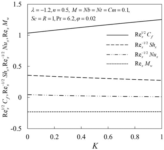
Figure 2.
.
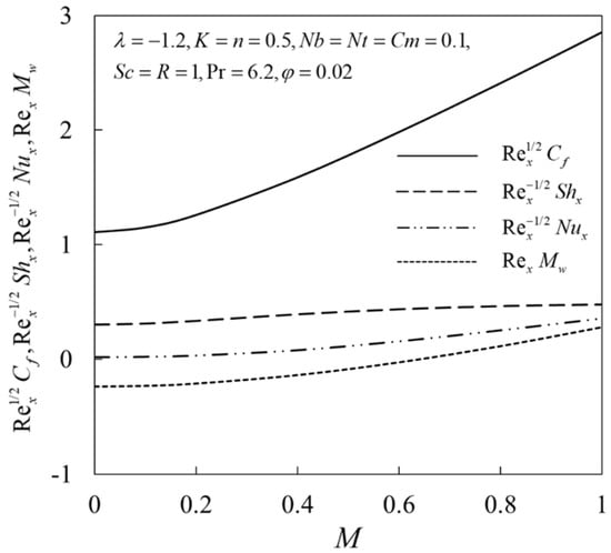
Figure 3.
.
Next, the variations in , , and against for water ( and Fe3O4/water when and are shown in Figure 4, Figure 5, Figure 6 and Figure 7, respectively. From these figures, it may be concluded that Fe3O4/water gives higher values of , , and for the first solution compared to water. The solution is unique when . Two solutions are obtained for the limited range of when the sheet is shrunk . Moreover, the solutions bifurcate and terminate in this region at (critical value), and this point is known as the bifurcation point. No solution is found beyond this value. Here, the critical values are for water ( and Fe3O4/water , respectively. This behavior is expected to occur because the addition of nanoparticles contributes to enhancing the thermal properties of fluids owing to the synergetic effects of nanoparticles.
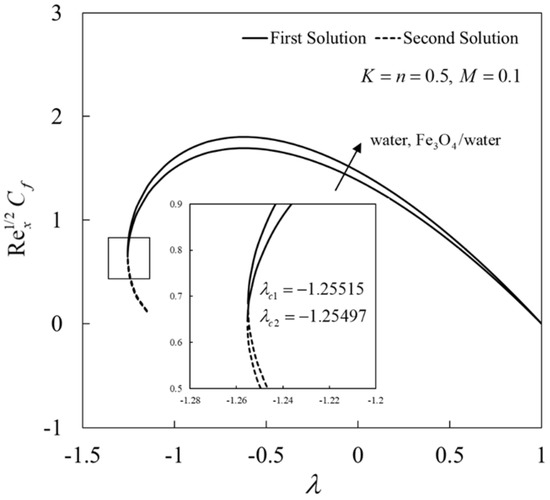
Figure 4.
for water and Fe3O4/water.
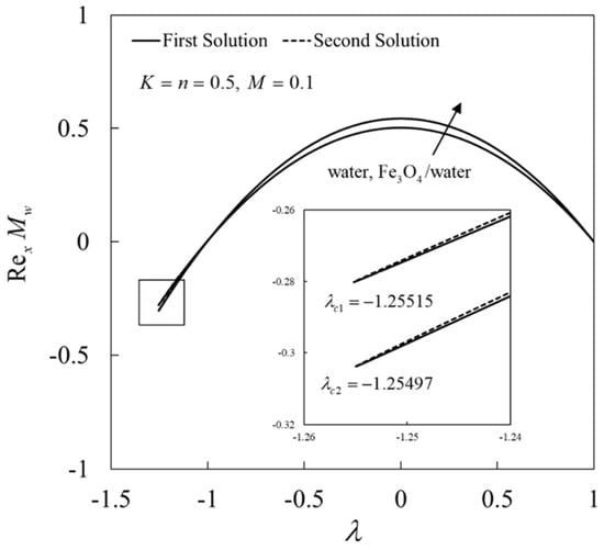
Figure 5.
for water and Fe3O4/water.
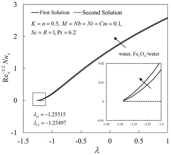
Figure 6.
for water and Fe3O4/water.
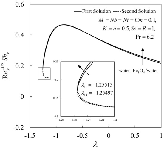
Figure 7.
for water and Fe3O4/water.
The influences of on the velocity , the microrotation , the temperature , and the concentration profiles when are presented in Figure 8, Figure 9, Figure 10 and Figure 11. Dual solutions exist that can be seen from these profiles, where both satisfy the infinity boundary conditions (14) asymptotically. Figure 8 and Figure 9 show that the velocity and the microrotation on both solutions decline for larger . Physically, the effect of microrotation is neglected when . On the other hand, the effects of the vortex and the dynamic viscosities are taken into account as increases. Therefore, the velocity decreases by thickening the momentum boundary layer. Moreover, it is interesting to note that the microrotation profiles experience the undershoot behavior near the shrinking sheet. This is because of the reverse movement of the sheet toward the origin. The microrotation increases near the sheet for larger K and then decreases when reaching the ambient condition. This observation has also been reported by Ishak et al. [13], Yacob and Ishak [14], and Soid et al. [15]. In contrast, the outcomes are the opposite for and , as shown in Figure 10 and Figure 11, where their boundary layer thicknesses are rising as K increases, consequently reducing the heat and the mass transfer.
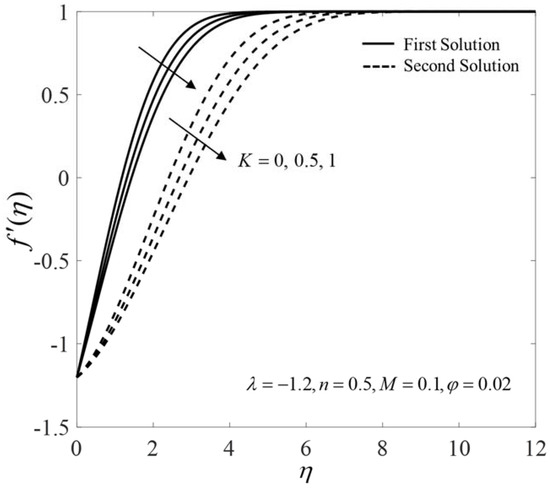
Figure 8.
Velocity for different values.
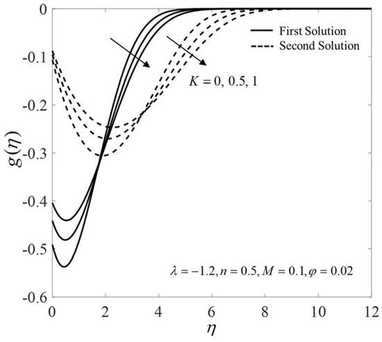
Figure 9.
The plot of for various values.
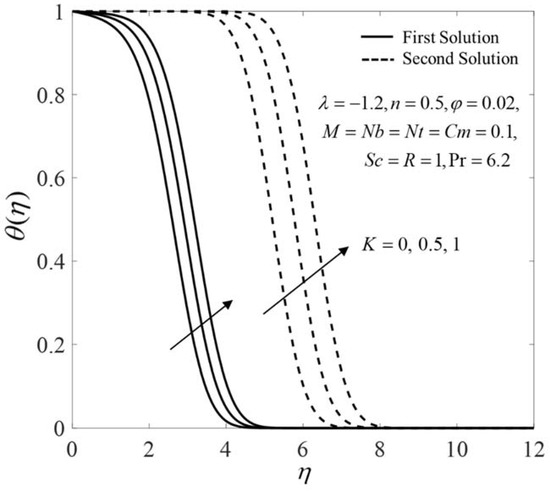
Figure 10.
Temperature for different values.
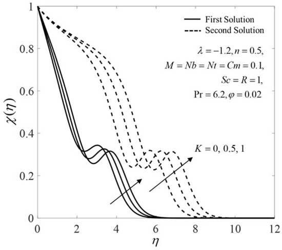
Figure 11.
The plot of for different values.
Figure 12 shows the streamlines when (stretching sheet), and . Meanwhile, Figure 13 and Figure 14 display the streamlines when (shrinking sheet), and for the first outcome and the second outcome, respectively. From Figure 12, the pattern of the streamlines is simple for the stretching case. A horizontal line divides the streamlines into two patterns for the shrinking case. This horizontal line is nearer to the shrinking region for the first solution compared to that of the second solution. It is also observed that the flow pattern in the upper region for the shrinking case is similar to that obtained for the stretching case. The reverse rotating flow is observed in the lower region.
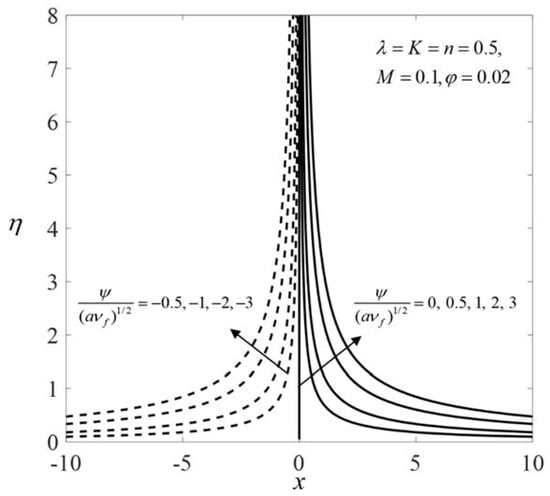
Figure 12.
Streamlines when (stretching sheet).
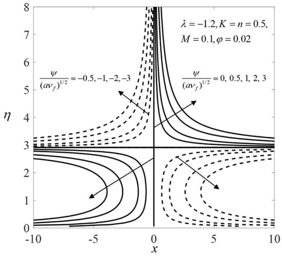
Figure 13.
Streamlines when (shrinking sheet) for the first solution.
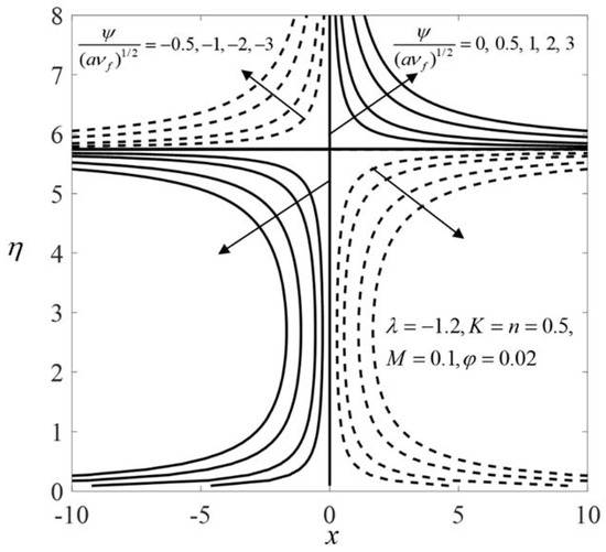
Figure 14.
Streamlines when (shrinking sheet) for the second solution.
The variation in against when is presented in Figure 15. It is noted that as time evolves for positive values of . On the other side, for the negative values of , . These observations show that the first solution is stable and thus physically reliable in the long run, and vice versa.
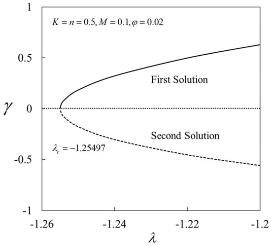
Figure 15.
Smallest eigen values of .
5. Conclusions
We investigated the micropolar fluid flow in a stagnation region of a stretching or shrinking sheet filled with Fe3O4 nanoparticles. The transformed equations were solved numerically by utilizing the bvp4c package in MATLAB software. The numerical outcomes are in agreement with previously published data. The findings reveal that two solutions are found for the limited range of the shrinking strength . The solutions bifurcate in this region at . Meanwhile, the solution is unique when . The physical quantities , , and increase with the rise in . Moreover, the effect of is found to lower the values of and but lead to an increase in the values of and . Furthermore, Fe3O4/water gives higher values of , , and compared to the base fluid, water. The critical values obtained in this study are beneficial in predicting the quality of certain products according to the desired output. We believe that this numerical study can be used in research on real applications. In future work, the present problem can be extended to examine the hybrid nanoparticles’ effect subjected to other flow conditions. Moreover, there are several physical parameters that can be examined regarding their effect on the flow and thermal behavior of the fluid.
Author Contributions
Formulation of mathematical model and methodology, I.W. and Y.Y.L.; Model validation, I.W.; Writing, I.W., Y.Y.L. and A.I.; review and editing, A.I. and I.P. All authors have read and agreed to the published version of the manuscript.
Funding
This research was funded by Universiti Kebangsaan Malaysia (project code: DIP-2020-001).
Acknowledgments
The financial support received from the Universiti Kebangsaan Malaysia (project code: DIP-2020-001) and the Universiti Teknikal Malaysia Melaka are gratefully acknowledged.
Conflicts of Interest
The authors declare no conflict of interest.
Nomenclature
| a, b | constants |
| B0 | strength of magnetic field (T) |
| C | concentration (mol m−3) |
| Cf | skin friction coefficient |
| Cm | chemical reaction parameter |
| cp | specific heat at constant pressure (J kg−1 K−1) |
| concentration at the surface (mol m−3) | |
| Brownian motion coefficient (m2 s−1) | |
| thermophoretic diffusion coefficient (mol m−1 s−1) | |
| dimensionless stream function | |
| dimensionless microrotation velocity | |
| microinertia coefficient (m2) | |
| material parameter | |
| mean absorption coefficient (m−1) | |
| thermal conductivity of the fluid (Wm−1 K−1) | |
| magnetic parameter | |
| local couple stress | |
| n | the micro-gyration parameter |
| N | microrotation velocity (s−1) |
| Nb | Brownian motion parameter |
| Nt | thermophoresis parameter |
| local Nusselt number | |
| Pr | Prandtl number |
| R | radiation parameter |
| Sc | Schmidt number |
| local Sherwood number | |
| T | fluid temperature (K) |
| Tw | surface temperature (K) |
| ambient temperature (K) | |
| u,v | components of velocity (m s−1) |
| x,y | Cartesian coordinates (m) |
| Greek symbols | |
| 𝛽 | first-order chemical reaction rate (s−1) |
| effective heat capacity ratio (m3 mol−1) | |
| η | similarity variable |
| θ | dimensionless temperature |
| vortex viscosity (kg m−1 s−1) | |
| λ | stretching/shrinking parameter |
| μ | dynamic viscosity (kg m−1 s−1) |
| ν | kinematic viscosity of the fluid (m2 s−1) |
| ρ | fluid density (kg m−3) |
| σ | electrical conductivity (S m−1) |
| σ∗ | Stefan–Boltzmann constant (W m−2 K−4) |
| nanoparticles volume fraction | |
| dimensionless concentration | |
| stream function (m2 s−1) | |
| ω | microinertia coefficient (kg m s−1) |
| Subscripts | |
| f | fluid |
| n | solid |
| nf | nanofluid |
| w | condition at the surface |
| Superscript | |
| ’ | differentiation with respect to η |
References
- Choi, S.U.S.; Eastman, J.A. Enhancing thermal conductivity of fluids with nanoparticles. In Proceedings of the 1995 International Mechanical Engineering Congress and Exhibition, San Francisco, CA, USA, 12–17 November 1995. [Google Scholar]
- Khanafer, K.; Vafai, K.; Lightstone, M. Buoyancy-driven heat transfer enhancement in a two-dimensional enclosure utilizing nanofluids. Int. J. Heat Mass Transf. 2003, 46, 3639–3653. [Google Scholar] [CrossRef]
- Tiwari, R.K.; Das, M.K. Heat transfer augmentation in a two-sided lid-driven differentially heated square cavity utilizing nanofluids. Int. J. Heat Mass Transf. 2007, 50, 2002–2018. [Google Scholar] [CrossRef]
- Oztop, H.F.; Abu-Nada, E. Numerical study of natural convection in partially heated rectangular enclosures filled with nanofluids. Int. J. Heat Fluid Flow 2008, 29, 1326–1336. [Google Scholar] [CrossRef]
- Jana, S.; Salehi-Khojin, A.; Zhong, W.H. Enhancement of fluid thermal conductivity by the addition of single and hybrid nano-additives. Thermochim. Acta 2007, 462, 45–55. [Google Scholar] [CrossRef]
- Suresh, S.; Venkitaraj, K.P.; Selvakumar, P.; Chandrasekar, M. Synthesis of Al2O3-Cu/water hybrid nanofluids using two step method and its thermo physical properties. Colloids Surf. A Physicochem. Eng. Asp. 2011, 388, 41–48. [Google Scholar] [CrossRef]
- Waini, I.; Ishak, A.; Pop, I. Squeezed hybrid nanofluid flow over a permeable sensor surface. Mathematics 2020, 8, 898. [Google Scholar] [CrossRef]
- Waini, I.; Ishak, A.; Pop, I. Mixed convection flow over an exponentially stretching/shrinking vertical surface in a hybrid nanofluid. Alex. Eng. J. 2020, 59, 1881–1891. [Google Scholar] [CrossRef]
- Waini, I.; Ishak, A.; Pop, I. Dufour and soret effects on al2o3-water nanofluid flow over a moving thin needle: Tiwari and das model. Int. J. Numer. Methods Heat Fluid Flow 2021, 31, 766–782. [Google Scholar] [CrossRef]
- Khashi’ie, N.S.; Waini, I.; Zainal, N.A.; Hamzah, K. Hybrid nanofluid flow past a shrinking cylinder with prescribed surface heat flux. Symmetry 2020, 12, 1493. [Google Scholar] [CrossRef]
- Eringen, A. Theory of micropolar fluids. J. Math. Mech. 1966, 16, 1–18. [Google Scholar] [CrossRef]
- Eringen, A.C. Theory of thermomicrofluids. J. Math. Anal. Appl. 1972, 38, 480–496. [Google Scholar] [CrossRef]
- Ishak, A.; Lok, Y.Y.; Pop, I. Stagnation-point flow over a shrinking sheet in a micropolar fluid. Chem. Eng. Commun. 2010, 197, 1417–1427. [Google Scholar] [CrossRef]
- Yacob, N.A.; Ishak, A. Stagnation point flow towards a stretching/shrinking sheet in a micropolar fluid with a convective surface boundary condition. Can. J. Chem. Eng. 2012, 90, 621–626. [Google Scholar] [CrossRef]
- Soid, S.K.; Ishak, A.; Pop, I. MHD stagnation-point flow over a stretching/shrinking sheet in a micropolar fluid with a slip boundary. Sains Malays. 2018, 47, 2907–2916. [Google Scholar] [CrossRef]
- Lok, Y.Y.; Amin, N.; Campean, D.; Pop, I. Steady mixed convection flow of a micropolar fluid near the stagnation point on a vertical surface. Int. J. Numer. Methods Heat Fluid Flow 2005, 15, 654–670. [Google Scholar] [CrossRef]
- Lok, Y.Y.; Pop, I.; Ingham, D.B.; Amin, N. Mixed convection flow of a micropolar fluid near a non-orthogonal stagnation-point on a stretching vertical sheet. Int. J. Numer. Methods Heat Fluid Flow 2009, 19, 459–483. [Google Scholar] [CrossRef]
- El-Aziz, M.A. Viscous dissipation effect on mixed convection flow of a micropolar fluid over an exponentially stretching sheet. Can. J. Phys. 2009, 87, 359–368. [Google Scholar] [CrossRef]
- Zaimi, W.M.K.A.W.; Ishak, A. Stagnation flow of a micropolar fluid towards a vertical permeable surface with prescribed heat flux. Sains Malays. 2012, 41, 1263–1270. [Google Scholar]
- Turkyilmazoglu, M. Mixed convection flow of magnetohydrodynamic micropolar fluid due to a porous heated/cooled deformable plate: Exact solutions. Int. J. Heat Mass Transf. 2017, 106, 127–134. [Google Scholar] [CrossRef]
- Khashi’ie, N.S.; Arifin, N.M.; Nazar, R.; Hafidzuddin, E.H.; Wahi, N.; Pop, I. Mixed convective flow and heat transfer of a dual stratified micropolar fluid induced by a permeable stretching/shrinking sheet. Entropy 2019, 21, 1162. [Google Scholar] [CrossRef]
- Ramadevi, B.; Anantha Kumar, K.; Sugunamma, V.; Ramana Reddy, J.V.; Sandeep, N. Magnetohydrodynamic mixed convective flow of micropolar fluid past a stretching surface using modified fourier’s heat flux model. J. Therm. Anal. Calorim. 2020, 139, 1379–1393. [Google Scholar] [CrossRef]
- Buongiorno, J. Convective transport in nanofluids. J. Heat Transf. 2006, 128, 240–250. [Google Scholar] [CrossRef]
- Hsiao, K.L. Micropolar nanofluid flow with MHD and viscous dissipation effects towards a stretching sheet with multimedia feature. Int. J. Heat Mass Transf. 2017, 112, 983–990. [Google Scholar] [CrossRef]
- Anwar, M.I.; Shafie, S.; Hayat, T.; Shehzad, S.A.; Salleh, M.Z. Numerical study for MHD stagnation-point flow of a micropolar nanofluid towards a stretching sheet. J. Braz. Soc. Mech. Sci. Eng. 2017, 39, 89–100. [Google Scholar] [CrossRef]
- Hayat, T.; Khan, M.I.; Waqas, M.; Alsaedi, A.; Khan, M.I. Radiative flow of micropolar nanofluid accounting thermophoresis and brownian moment. Int. J. Hydrogen Energy 2017, 42, 16821–16833. [Google Scholar] [CrossRef]
- Ibrahim, W. Passive control of nanoparticle of micropolar fluid past a stretching sheet with nanoparticles, convective boundary condition and second-order slip. Proc. Inst. Mech. Eng. Part E J. Process Mech. Eng. 2017, 231, 704–719. [Google Scholar] [CrossRef]
- Siddiq, M.K.; Rauf, A.; Shehzad, S.A.; Abbasi, F.M.; Meraj, M.A. Thermally and solutally convective radiation in mhd stagnation point flow of micropolar nanofluid over a shrinking sheet. Alex. Eng. 2018, 57, 963–971. [Google Scholar] [CrossRef]
- Kumar, B.; Seth, G.S.; Nandkeolyar, R. Regression model and successive linearization approach to analyse stagnation point micropolar nanofluid flow over a stretching sheet in a porous medium with nonlinear thermal radiation. Phys. Scr. 2019, 94, 115211. [Google Scholar] [CrossRef]
- Patel, H.R.; Singh, R. Thermophoresis, brownian motion and non-linear thermal radiation effects on mixed convection mhd micropolar fluid flow due to nonlinear stretched sheet in porous medium with viscous dissipation, joule heating and convective boundary condition. Int. Commun. Heat Mass Transf. 2019, 107, 68–92. [Google Scholar] [CrossRef]
- Zaib, A.; Khan, U.; Shah, Z.; Kumam, P.; Thounthong, P. Optimization of entropy generation in flow of micropolar mixed convective magnetite (Fe3O4) ferroparticle over a vertical plate. Alex. Eng. J. 2019, 58, 1461–1470. [Google Scholar] [CrossRef]
- Ghadikolaei, S.S.; Hosseinzadeh, K.; Hatami, M.; Ganji, D.D. MHD boundary layer analysis for micropolar dusty fluid containing hybrid nanoparticles (Cu-Al2O3) over a porous medium. J. Mol. Liq. 2018, 268, 813–823. [Google Scholar] [CrossRef]
- Subhani, M.; Nadeem, S. Numerical analysis of micropolar hybrid nanofluid. Appl. Nanosci. 2019, 9, 447–459. [Google Scholar] [CrossRef]
- Subhani, M.; Nadeem, S. Numerical investigation into unsteady magnetohydrodynamics flow of micropolar hybrid nanofluid in porous medium. Phys. Scr. 2019, 94, 105220. [Google Scholar] [CrossRef]
- Al-Hanaya, A.M.; Sajid, F.; Abbas, N.; Nadeem, S. Effect of SWCNT and MWCNT on the flow of micropolar hybrid nanofluid over a curved stretching surface with induced magnetic field. Sci. Rep. 2020, 10, 8488. [Google Scholar] [CrossRef]
- Hosseinzadeh, K.; Roghani, S.; Asadi, A.; Mogharrebi, A.; Ganji, D.D. Investigation of micropolar hybrid ferro fluid flow over a vertical plate by considering various base fluid and nanoparticle shape factor. Int. J. Numer. Methods Heat Fluid Flow 2020, 31, 402–417. [Google Scholar] [CrossRef]
- Uddin, M.J.; Kabir, M.N.; Alginahi, Y.M. Lie group analysis and numerical solution of magnetohydrodynamic free convective slip flow of micropolar fluid over a moving plate with heat transfer. Comput. Math. Appl. 2015, 70, 846–856. [Google Scholar] [CrossRef]
- Zohra, F.T.; Uddin, M.J.; Ismail, A.I.M. Magnetohydrodynamic bio-nanoconvective naiver slip flow of micropolar fluid in a stretchable horizontal channel. Heat Transf. Asian Res. 2019, 48, 3636–3656. [Google Scholar] [CrossRef]
- Abdul Latiff, N.A.; Uddin, M.J.; Bég, O.A.; Ismail, A.I. Unsteady forced bioconvection slip flow of a micropolar nanofluid from a stretching/shrinking sheet. Proc. Inst. Mech. Eng. Part N J. Nanomater. Nanoeng. Nanosyst. 2016, 230, 177–187. [Google Scholar] [CrossRef]
- Uddin, M.J.; Bég, O.A.; Ismail, A.I. Radiative convective nanofluid flow past a stretching/shrinking sheet with slip effects. J. Thermophys. Heat Transf. 2015, 29, 513–523. [Google Scholar] [CrossRef]
- Rana, B.M.J.; Arifuzzaman, S.M.; Islam, S.; Reza-E-Rabbi, S.; Hossain, K.E.; Ahmmed, S.F.; Khan, M.S. Swimming of microbes in entropy optimized nano-bioconvective flow of prandtl–erying fluid. Heat Transf. 2022, 51, 5497–5531. [Google Scholar] [CrossRef]
- Khan, W.A.; Ali, M.; Waqas, M.; Shahzad, M.; Sultan, F.; Irfan, M. Importance of convective heat transfer in flow of non-newtonian nanofluid featuring brownian and thermophoretic diffusions. Int. J. Numer. Methods Heat Fluid Flow 2019, 29, 4624–4641. [Google Scholar] [CrossRef]
- Khan, W.A.; Farooq, S.; Kadry, S.; Hanif, M.; Iftikhar, F.J.; Abbas, S.Z. Variable characteristics of viscosity and thermal conductivity in peristalsis of magneto-carreau nanoliquid with heat transfer irreversibilities. Comput. Methods Programs Biomed. 2020, 190, 105355. [Google Scholar] [CrossRef]
- Khan, W.A.; Waqas, M.; Chammam, W.; Asghar, Z.; Nisar, U.A.; Abbas, S.Z. Evaluating the characteristics of magnetic dipole for shear-thinning williamson nanofluid with thermal radiation. Comput. Methods Programs Biomed. 2020, 191, 105396. [Google Scholar] [CrossRef] [PubMed]
- Khan, W.A.; Ali, M.; Irfan, M.; Khan, M.; Shahzad, M.; Sultan, F. A rheological analysis of nanofluid subjected to melting heat transport characteristics. Appl. Nanosci. 2020, 10, 3161–3170. [Google Scholar] [CrossRef]
- Patel, H.R.; Mittal, A.S.; Darji, R.R. MHD flow of micropolar nanofluid over a stretching/shrinking sheet considering radiation. Int. Commun. Heat Mass Transf. 2019, 108, 104322. [Google Scholar] [CrossRef]
- Waini, I.; Ishak, A.; Pop, I. Hybrid nanofluid flow past a permeable moving thin needle. Mathematics 2020, 8, 612. [Google Scholar] [CrossRef]
- Yahaya, R.I.; Arifin, N.M.; Nazar, R.; Pop, I. Flow and heat transfer past a permeable stretching/shrinking sheet in Cu−Al2O3/water hybrid nanofluid. Int. J. Numer. Methods Heat Fluid Flow 2020, 30, 1197–1222. [Google Scholar] [CrossRef]
- Sulochana, C.; Aparna, S.R. Unsteady magnetohydrodynamic radiative liquid thin film flow of hybrid nanofluid with thermophoresis and brownian motion. Multidiscip. Modeling Mater. Struct. 2020, 16, 811–834. [Google Scholar] [CrossRef]
- Rana, P.; Shukla, N.; Bég, O.A.; Bhardwaj, A. lie group analysis of nanofluid slip flow with stefan blowing effect via modified buongiorno’s model: Entropy generation analysis. Differ. Equ. Dyn. Syst. 2021, 29, 193–210. [Google Scholar] [CrossRef]
- Mahanthesh, B.; Shehzad, S.A.; Mackolil, J.; Shashikumar, N.S. Heat transfer optimization of hybrid nanomaterial using modified buongiorno model: A sensitivity analysis. Int. J. Heat Mass Transf. 2021, 171, 121081. [Google Scholar] [CrossRef]
- Clancy, L.J. Aerodynamics; Pitman Publishing: London, UK, 1975. [Google Scholar]
- Borrelli, A.; Giantesio, G.; Patria, M.C. An exact solution for the 3D MHD stagnation-point flow of a micropolar fluid. Commun. Nonlinear Sci. Numer. Simul. 2015, 20, 121–135. [Google Scholar] [CrossRef]
- Pritchard, P.J.; Leylegian, J.C. Fox and McDonald’s Introduction to Fluid Mechanics; John Wiley & Sons, Inc.: Hoboken, NJ, USA, 2011; ISBN 9780470547557. [Google Scholar]
- Wang, C.Y. Stagnation flow towards a shrinking sheet. Int. J. Non-Linear Mech. 2008, 43, 377–382. [Google Scholar] [CrossRef]
- Hartmann, J. Hg-dynamics I. Theory of the laminar conductive liquid in a homogeneous magnetic field. Det Kgl. Dan. Vidensk. Selskab. Math. Fys. Medd. 1937, 15, 1–28. [Google Scholar]
- Pavlov, K.B. Magnetohydrodynamics flow of an incompressible viscous liquid caused by deformation of plane surface. Magnetohydrodynamics 1974, 10, 507–510. [Google Scholar]
- Ibrahim, W.; Shankar, B.; Nandeppanavar, M.M. MHD stagnation point flow and heat transfer due to nanofluid towards a stretching sheet. Int. J. Heat Mass Transf. 2013, 56, 1–9. [Google Scholar] [CrossRef]
- Ajith Krishnan, R.; Jinshah, B.S. Magnetohydrodynamic power generation. Int. J. Sci. Res. Publ. 2013, 3, 1–11. [Google Scholar] [CrossRef]
- Modest, M.F. Radiative Heat Transfer, 3rd ed.; Academic Press: Oxford, UK, 2013. [Google Scholar]
- Rosseland, S. Astrophysik und Atom-Theoretische Grundlagen; Springer: Berlin/Heidelberg, Germany, 1931; ISBN 9783662245330. [Google Scholar]
- Howell, J.R.; Siegel, R.; Mengüç, M.P. Thermal Radiation Heat Transfer, 5th ed.; CRC Press, Taylor & Fracis Group: Boca Raton, FL, USA, 2010; ISBN 9781466593275. [Google Scholar]
- Muthtamilselvan, M.; Ramya, E.; Doh, D.H. Inclined lorentz force effects on 3d micropolar fluid flow due to a stretchable rotating disks with higher order chemical reaction. Proc. Inst. Mech. Eng. Part C J. Mech. Eng. Sci. 2019, 233, 323–335. [Google Scholar] [CrossRef]
- Rawat, S.K.; Upreti, H.; Kumar, M. Comparative study of mixed convective MHD cu-water nanofluid flow over a cone and wedge using modified buongiorno’s model in presence of thermal radiation and chemical reaction via cattaneo-christov double diffusion model. J. Appl. Comput. Mech. 2021, 7, 1383–1402. [Google Scholar] [CrossRef]
- Singh, K.; Pandey, A.K.; Kumar, M. Numerical solution of micropolar fluid flow via stretchable surface with chemical reaction and melting heat transfer using keller-box method. Propuls. Power Res. 2021, 10, 194–207. [Google Scholar] [CrossRef]
- Xiong, P.Y.; Chu, Y.M.; Ijaz Khan, M.; Khan, S.A.; Abbas, S.Z. Entropy optimized darcy-forchheimer flow of reiner-philippoff fluid with chemical reaction. Comput. Theor. Chem. 2021, 1200, 113222. [Google Scholar] [CrossRef]
- Merkin, J.H. On dual solutions occurring in mixed convection in a porous medium. J. Eng. Math. 1986, 20, 171–179. [Google Scholar] [CrossRef]
- Weidman, P.D.; Kubitschek, D.G.; Davis, A.M.J. The effect of transpiration on self-similar boundary layer flow over moving surfaces. Int. J. Eng. Sci. 2006, 44, 730–737. [Google Scholar] [CrossRef]
- Harris, S.D.; Ingham, D.B.; Pop, I. Mixed convection boundary-layer flow near the stagnation point on a vertical surface in a porous medium: Brinkman model with slip. Transp. Porous Media 2009, 77, 267–285. [Google Scholar] [CrossRef]
- Shampine, L.F.; Gladwell, I.; Thompson, S. Solving ODEs with MATLAB; Cambridge University Press: Cambridge, UK, 2003; ISBN 9780521824040. [Google Scholar]
- Pantokratoras, A. A common error made in investigation of boundary layer flows. Appl. Math. Model. 2009, 33, 413–422. [Google Scholar] [CrossRef]
Publisher’s Note: MDPI stays neutral with regard to jurisdictional claims in published maps and institutional affiliations. |
© 2022 by the authors. Licensee MDPI, Basel, Switzerland. This article is an open access article distributed under the terms and conditions of the Creative Commons Attribution (CC BY) license (https://creativecommons.org/licenses/by/4.0/).