Article

Bilateral Feedback in Oscillator Model Is Required to Explain the Coupling Dynamics of Hes1 with the Cell Cycle

1
Division of Developmental Biology and Medicine, School of Medical Sciences, Faculty of Biology, Medicine and Health (FBMH), The University of Manchester, Oxford Road, Manchester M13 9PT, UK
2
Unit 2 & 2a, Enterprise House, Lloyd Street North, Manchester M15 6SE, UK
*
Author to whom correspondence should be addressed.
Mathematics 2022, 10(13), 2323; https://doi.org/10.3390/math10132323
Submission received: 27 May 2022 / Revised: 25 June 2022 / Accepted: 28 June 2022 / Published: 2 July 2022
(This article belongs to the Section Difference and Differential Equations)

Abstract

:
Biological processes are governed by the expression of proteins, and for some proteins, their level of expression can fluctuate periodically over time (i.e., they oscillate). Many oscillatory proteins (e.g., cell cycle proteins and those from the HES family of transcription factors) are connected in complex ways, often within large networks. This complexity can be elucidated by developing intuitive mathematical models that describe the underlying critical aspects of the relationships between these processes. Here, we provide a mathematical explanation of a recently discovered biological phenomenon: the phasic position of the gene Hes1’s oscillatory expression at the beginning of the cell cycle of an individual human breast cancer stem cell can have a predictive value on how long that cell will take to complete a cell cycle. We use a two-component model of coupled oscillators to represent Hes1 and the cell cycle in the same cell with minimal assumptions. Inputting only the initial phase angles, we show that this model is capable of predicting the dynamic mitosis to mitosis behaviour of Hes1 and predicting cell cycle length patterns as found in real-world experimental data. Moreover, we discover that bidirectional coupling between Hes1 and the cell cycle is critical within the system for the data to be reproduced and that nonfixed asymmetry in the interactions between the oscillators is required. The phase dynamics we present here capture the complex interplay between Hes1 and the cell cycle, helping to explain nongenetic cell cycle variability, which has critical implications in cancer treatment contexts.

1. Introduction

The transcription, translation and, ultimately, protein assembly of a specific gene is known as its gene expression. The temporal dynamics of gene expression are known to be a key factor in determining cell fate in many contexts [1,2,3]. Biological and technical advances (e.g., in fluorescent protein reporters and microscopy [4]) have meant that dynamic data has become increasingly abundant (for example, reviewed in [5]), yet dynamic gene expression remains difficult to measure and interpret [6,7,8].
The cell cycle is a biological process during which a cell undergoes an ordered series of predetermined procedures and checks, culminating in its division into two cells [9]. It has been well understood through the lens of gene expression and post-transcriptional dynamics that there are many proteins (e.g., cyclins) whose abundance peaks once and at specific times in each cell cycle [10,11] (Figure 1A bottom panel). It is also known that the cell cycle is closely linked to cell fate [12,13,14]. Hes1 (hairy and enhancer of split-1) is a transcription factor (TF) protein that is encoded by the Hes1 gene in mammals; it is known to regulate cell fate [15,16,17,18,19] but also interferes with the cell cycle through repression of cell cycle-related proteins [20,21,22]. Hes1 is also known to be important in cancer [23,24]; for example, it has been shown that elevation of Hes1 can contribute to cancer metastasis, and Hes1 overexpression can even lead to drug resistance [25].
In [26], we used single-cell live imaging to track Hes1 expression in a human ER+ breast cancer cell (BCC) line, known as MCF-7 [27,28], which contains breast cancer stem cells (BCSCs) [29] alongside tumour bulk cells. We discovered that the Hes1 protein exhibits a large oscillatory pattern averaging a circadian-like periodicity (≈25 h), while an oscillatory pattern with a shorter periodicity (≈4 h) was found when this larger oscillatory trend was removed. These nested ultradian (shorter than one day but longer than one hour in periodicity) oscillations, which are caused by transcriptional self-repression, a well-researched characteristic of Hes/Her genes [30,31,32], showed no correlation with the high levels of heterogeneity in cell cycle durations found in the MCF7 population. Conversely, the circadian-like oscillatory Hes1 trend within the cells did provide patterns related to longer and shorter cell cycles. We determined that it is the momentary position within these oscillations at the beginning of a cell’s life that has the greatest correlation with the eventual length of time taken before that cell divides (demonstrated in Figure 1). More specifically, when clustered by their Hes1 dynamics into three distinct groups, cells whose beginning mitoses were at or just after a trough in oscillation (cluster 3 as illustrated in Figure 1D) predominantly possessed longer cell cycles (Figure 1F) than those that began their life in a different part of the oscillatory wave (clusters 1 and 2 in Figure 1B,C). However, it remains unclear how this feature of Hes1 protein oscillations at the beginning of mitosis in a breast cancer cell results in specific mitosis to mitosis dynamics and, further, why this corresponds to distinguishable differences in cell cycle durations. Therefore, we ask why is it that our cluster 3 cells exhibit longer cell cycles and why do clusters 1 and 2 have similar and shorter cell cycle durations despite having different initial Hes1 dynamic behaviour? This paper aims to shed light on these questions.
Mathematics, and particularly dynamical systems theory, has had an impact on understanding gene expression dynamics [33,34,35] (specifically Hes1 dynamics [36,37,38,39]), the cell cycle [40,41,42,43,44,45] and their links to cell fate [46,47,48]. Although the relationship between Hes1 and cell cycle has previously been investigated in large, multiple parameter models (in [49], for example), thus far, no two-component (Hes1/cell cycle) model exists. Typically, models involving gene expression are very complicated and comprise vast multi-parameter spaces that are difficult to explore and relate to observations from real data. These models also require extensive experimental validation in order to verify the necessity of each component. Furthermore, we note that there has not yet been a study that models Hes1 dynamics with oscillations at the circadian scale, although coupled oscillator models such as [50,51] have been used to study circadian rhythms with the human sleep-wake cycle.
Our goal in this paper is to implement a minimal and thus, intelligible mathematical model in order to understand and make predictions on specifically the interaction between Hes1 and the cell cycle, which ideally can then reproduce the results in [26] (which are illustrated in Figure 1) without the need for many components. Discovery and critical evaluation of an intuitive mathematical explanation behind the relationship between the oscillatory expression of Hes1 and the cell cycle may provide clearer insight into the systems at play. By achieving this, one may be able to systematically probe this biological interaction via specifically designed experimentation. This can allow for causal effects between the two phenomena to be uncovered, resulting in a better understanding of the study of cell cycle elongation/dormancy, which, in a cancer context, may prove informative for clinical treatment.

2. Mathematical Modelling Strategy

While mathematical modelling approaches to gene expression dynamics often involve simulations of protein and/or mRNA abundances over time [52,53,54,55], we take the route of modelling the relative temporal progression of two coupled oscillators. By this, we mean mathematical models that are defined by systems of differential equations whereby the dependent variables each represent the phase angle of an oscillator. By “phase”, we mean the position at a given time, relative to some point of origin, within the progression of one cycle of a periodic object. We may define this mathematically as a real-valued angle θ 0 , 2 π of a point on the circumference of a circle from some predefined original point on the circumference. Models of this form have previously been applied to the cell cycle and the circadian clock oscillators in differing contexts in [56,57,58]: these publications provided particular inspiration for this paper. For the model we implement here, our two coupled oscillators shall be Hes1 gene expression dynamics (as described in [26] and displayed in Figure 1) and the cell cycle. Therefore, as such, we label our model variables as θ Hes1 and θ C . C . and periodic functions determining their temporal behaviour as f Hes1 , f C . C . .
The decision to model Hes1 as an oscillator is justified since it was found that gene expression of Hes1 is oscillatory (and corroborated via multiple methods) in [26] on a near circadian scale. It may be argued though, that the cell cycle ought not to be considered an oscillator (as is done in [59]) due to its series of discrete points in time: checkpoints, potential stoppage events, etc. However, we shall take a more simplified view and assume that processes such as cell differentiation, apoptosis and cell cycle arrest, etc., do not occur. This allows us to assume that each time a cell division occurs, a new cell cycle begins, and thus, cell division can be seen as a repeated, periodic event in time. For the purposes of a mathematical model, we may, therefore, consider the cell cycle process as a continuous oscillator (like in [60,61]) with an inherent periodicity: i.e., the time between divisions. Furthermore, here we shall take a more abstract view of the cell cycle checkpoint events themselves in that we do not make any assumptions on the specific durations of the biological cell cycle phases: G1, S, G2 [9,62], which are present within the cell cycle. The results from multiple control experiments in [26] also suggest that Hes1 and the cell cycle are coupled oscillators further justifies our approach.

2.1. Phase Representation of Bcc Data

When choosing the specifics of our intended model, i.e., the nature of functions f Hes1 and f C . C . , we examined the data we intend to model. One key aspect of the results from [26] is important here: in each case (Figure 1B–D), irrespective of the phase at the beginning of cell cycles, Hes1 invariably goes through a trough followed by an upward trend in dynamics before the cell cycle ends. This hints at a pattern forming between the phases of both oscillators as time progresses. To study instantaneous phase over time, our pseudo-time-series signals are plotted in Figure 1B–D respectively; we used hilbert.m and the angle.m functions in MATLAB. The function hilbert.m develops the analytic signal ξ ( t ) of a signal vector s , which is defined in [63] as
ξ ( t ) = s ( t ) + i s H = A ( t ) e i θ ( t )
where here, the function
s H ( t ) = π 1 s ( τ ) t τ d τ
is the Hilbert Transform of the signal vector s . In (1), A ( t ) is the signal’s instantaneous amplitude, and θ ( t ) is the instantaneous phase. The function angle.m used upon an analytic signal vector returns θ ( t ) as a vector (with the same length as s ) of real values modulo 2 π . The vector θ is now the estimated phase reconstruction of s . As an example, using functions hilbert.m followed by angle.m on a perfect sine wave will return a sawtooth wave. The phase reconstructions of the three clustered pseudo-time Hes1 signal traces (Figure 1B–D) are now vectors of length T Z + , which correspond to the position in the phase of each trace at all points in pseudo-time; we shall label them as Θ Hes1 ( i ) where i = 1 , 2 , 3 denotes the cluster mean traces from which they were derived. We may then plot these against a uniformly spaced cell-cycle phase vector ( Θ C . C . ) between 0 and 2 π of the same length to produce trajectories of our data in two-dimensional phase space. This phase space can then be drawn onto a square torus diagram (Figure 2B), where the phase of both oscillators are unfolded along the x and y-axes.
One noticeable feature in Figure 2 is that torus diagram trajectories of clusters 2 (blue line) and 3 (green line), despite beginning quite close together, appear to initially be moving away from each other as though repelled. Additionally, both trajectories, along with the cluster 1 trajectory (red line), appear to collect around a similar area (upper right-hand quadrant) in the phase space as the cell cycle oscillator phase angle reaches 2 π . This is also illustrated in Figure 2C, where in the far right-hand side column, all dots are close together around the top of the circle. This implies that in all cases, as the cell cycle reaches an end, the Hes1 oscillator is attracted to a particular phase. This indicates that a form of phase locking between the Hes1 and the cell cycle oscillators may exist. To that end, we choose the following model, which is known to exhibit this property.

2.2. Specifying the Coupled Oscillator Model

We model the interactions between cell cycle and Hes1 using the following previously characterised system of coupled oscillators in [64]:
d θ 1 d t = ω 1 + K 1 sin θ 2 θ 1 , d θ 2 d t = ω 2 + K 2 sin θ 1 θ 2 ,
where θ i is the phase of oscillator i, ω i is the free-running intrinsic frequency of oscillator i and K i is the strength of effect from oscillator j onto oscillator i for i , j = 1 , 2 and i j . This particular system of ordinary differential equations has previously been used to model circadian rhythms in humans [50,51], which makes it well-suited to be applied to our data since we see circadian-like Hes1 periodicity in human breast cancer stem cells in [26]. The above model is also an asymmetric, two-component version of the Kuramoto coupled oscillator model [65]. Although, in some cases, the Kuramoto model is used for purely theoretical studies, it has been previously used to good effect when used in conjunction with cell biology [66,67]. Analysis of the system Equation (3) will show that if K 1 , K 2 > 0 , then by considering the difference in phases between the oscillators ϕ = θ 1 θ 2 we get
d ϕ d t = d θ 1 d t d θ 2 d t = ω 1 ω 2 K 1 + K 2 sin ( ϕ ) .
This ODE has two fixed points i . e . , d ϕ d t = 0 when ω 1 ω 2 < K 1 + K 2 (shown by means of vector field diagrams in Equation (3)). Therefore, two phase-locked solutions will exist, one stable and one unstable, and the phase space trajectories will asymptotically approach the stable phase-locked solution in which both oscillators will run at a constant compromise frequency defined as
ω * = K 1 ω 2 + K 2 ω 1 K 1 + K 2
and be separated by a constant phase difference ϕ * [64]. These two phase-locked solutions will appear as diagonal lines with slope 1 when plotted on a square torus diagram and have also been called “attractor” and “repeller” lines in [57]. We now consider this model with the two oscillators representing Hes1 and the cell cycle; we aim to use this model to reproduce the phase data shown in Figure 2 and thus be able to find a mathematical explanation with the assistance of the previously-stated analysis. Examining Equation (3) closely makes us aware that an unwanted scenario may occur: suppose, for example, that θ 2 θ 1 = 3 π 2 then sin θ 2 θ 1 = 1 and constants ω 1 < K 1 , then we get d θ 1 d t < 0 . Now, we know that the cell cycle cannot backtrack in its progression [62]. Therefore, allowing this to occur in our model would be unrealistic; hence we shall ensure that rates d θ 1 d t , d θ 2 d t 0 , i.e., our oscillators may not progress backwards. We can impose this by using the following substitutions K 1 = ω 1 κ 1 , K 2 = ω 2 κ 2 , where κ 1 , κ 2 [ 0 , 1 ] . Applying these substitutions, factorising and replacing variable names to our specifications yields the model with which we shall continue:
d θ Hes1 d t = ω Hes1 1 + κ Hes1 sin θ C . C . θ Hes1 , d θ C . C . d t = ω C . C . 1 + κ C . C . sin θ Hes1 θ C . C . ,
where θ Hes1 , θ C . C . [ 0 , 2 π ) are continuous functions of time that represent the phase progression of Hes1 expression oscillations and the cell cycle, respectively. Constant parameters ω Hes1 > 0 and ω C . C . > 0 are the Hes1 and cell cycle oscillators’ intrinsic frequencies, respectively, and κ Hes1 is now a scaled coupling constant that represents the strength of effect that the cell cycle oscillator phase has upon the Hes1 phase and vice-versa for the parameter κ C . C . . These coupling strength parameters are currently unassigned, but we allow the possibility for either or both to be equal to zero, implying the scenario of no coupling or of unidirectional coupling, respectively. As per our earlier definition, we make the following arbitrary choices:
  • θ Hes1 = 0 will be considered the peak of an oscillatory Hes1 wave, and θ Hes1 = π is the trough.
  • θ C . C . = 0 will denote the beginning and the end of a cell cycle, i.e., a cell division event.

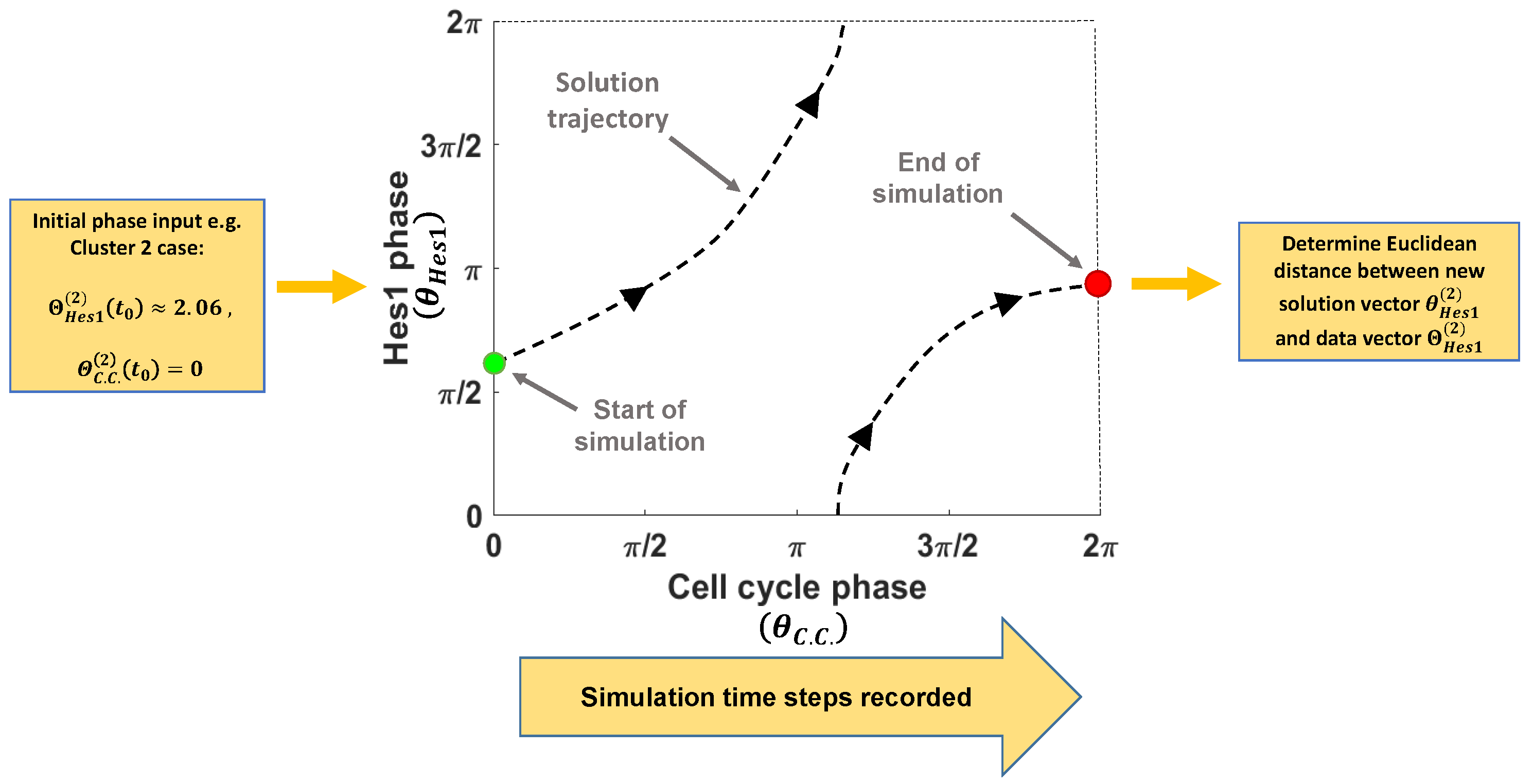
2.3. Numerical Implementation

In Section 3, the results are shown from our numerical simulations: solutions to the coupled system of Equation (5) are approximated in MATLAB via a fourth-order Runge-Kutta (RK) numerical scheme with a step-size of h = 0.1 . This scheme is described as follows: we set the cell cycle oscillator initial condition as θ C . C . ( t 0 ) = 0 (where t 0 is our initial time step) and set the Hes1 oscillator initial condition as one of the three initial phase values found from the phase reconstruction of the clustered Hes1 dynamics in the data: that is, θ Hes1 ( 1 ) ( t 0 ) = Θ Hes1 ( 1 ) ( 1 ) 6.0830 , θ Hes1 ( 2 ) ( t 0 ) = Θ Hes1 ( 2 ) ( 1 ) 2.0164 and θ Hes1 ( 3 ) ( t 0 ) = Θ Hes1 ( 3 ) ( 1 ) 3.3613 (these values correspond to the radial coloured lines in Figure 1E). We choose the constant intrinsic frequency parameter values ω Hes1 and ω C . C . to be the reciprocals of the median Hes1 periodicity (24 h) and the median cell cycle length estimates (27 h), respectively, from the dataset of 164 BCCs found in [26]. At the nth iteration of the numerical scheme, we have the functions
f Hes1 ( t n , θ Hes1 ( t n ) , θ C . C . ( t n ) ) = ω Hes1 ( 1 + κ Hes1 sin θ C . C . ( t n ) θ Hes1 ( t n ) ) , f C . C . ( t n , θ Hes1 ( t n ) , θ C . C . ( t n ) ) = ω C . C . ( 1 + κ C . C . sin θ Hes1 ( t n ) θ C . C . ( t n ) ) .
Each time step iteration is determined by
θ Hes1 t n + 1 = θ Hes1 t n + 1 6 h k 1 Hes1 . + 2 k 2 Hes1 . + 2 k 3 Hes1 + k 4 Hes1 , θ C . C . t n + 1 = θ C . C . t n + 1 6 h k 1 C . C . + 2 k 2 C . C . + 2 k 3 C . C . + k 4 C . C . , t n + 1 = t n + h ,
where
k 1 i = f i t n , θ i ( t n ) , θ j t n , k 2 i = f i t n + h 2 , θ i ( t n ) + h k 1 i 2 , θ j ( t n ) + h k 1 i 2 , k 3 i = f i t n + h 2 , θ i ( t n ) + h k 2 i 2 , θ j ( t n ) + h k 2 i 2 , k 4 i = f i t n + h , θ i ( t n ) + h k 3 i , θ j ( t n ) + h k 3 i ,
for n = 0 , 1 , 2 , , i , j = Hes1 , C . C . and i j . We consider one simulation to be complete at the time point t m , m Z + at which θ C . C . ( t m ) < 2 π and θ C . C . ( t m + 1 ) > 2 π . This value of t m is recorded and the solution vectors θ Hes1 ( i ) , i = 1 , 2 , 3 are then interpolated into pseudo-time (a vector of length T) and compared against their corresponding data vector ( Θ Hes1 ( i ) , i = 1 , 2 , 3 ) as described in Section 2.4. Since κ Hes1 and κ C . C . are unknown parameters, the simulations are run many times over a finely gridded ( 100 × 100 ) parameter space of κ Hes1 × κ C . C . . This process is illustrated in the schematic in Figure 3.

2.4. Model Optimisation Strategy

We are interested in determining at which points in the parameter space κ Hes1 × κ C . C . our model is most successful at fitting the data. In a further test of the system, we shall impose a number of different parameter constraints (unidirectional coupling, symmetric coupling and (for completeness) no coupling) to investigate whether the data is reproducible with a more restricted model. These constraints will give us additional insight into the directionality of interaction between Hes1 and the cell cycle.
The success of our model is judged two-fold: first, it is determined by residual error (Euclidean distance) in the model solution vectors ( θ Hes1 ) and data vectors ( Θ Hes1 ); the smaller the error, the better the fit. Secondly, we can record the number of time steps ( t m ) required for our model to complete one cell cycle simulation. Of course, these outputs are measured in iterative time steps and thus cannot directly correspond back to real-time cell cycle duration estimates. However, we may gauge the accuracy of our model by comparing these simulated predictions between cluster cases, similar to the bar chart in Figure 1F. The latter of these success gauges is the most interesting since we are only parameterising our model to fit the time-independent Θ Hes1 dynamics.
We may write out our optimisation problem more formally in the following manner:
minimise κ Hes1 , κ C . C . R ( κ Hes1 , κ C . C . ) subject to Strategy 2 : κ Hes1 = κ C . C . , or Strategy 3 : 0 κ Hes1 1 , κ C . C . = 0 , or Strategy 4 : κ Hes1 = 0 , 0 κ C . C . 1 , or Strategy 5 : 0 κ Hes1 1 , 0 κ C . C . 1 .
where
R ( κ Hes1 , κ C . C . ) = j = 1 T Θ Hes1 ( i ) ( j ) θ Hes1 ( i ) ( j ) 2 , for i = 1 , 2 , 3 .
Our resulting figures in the next section will illustrate square torus diagrams with trajectories for the best fit of our model found to the data for each parameter constraint. The resulting figures will also display the rebuilt Hes1 dynamics from that simulation: these are produced by inputting the resulting θ Hes1 solution vector into a cosine function that acts as the inverse action to the use of the Hilbert transform discussed earlier. Finally, they will show a bar chart of the t end values recorded for the optimally fitted models. We emphasise here that a good result from our model to the data will have:
  • A low residual fit (R) value.
  • A torus diagram trajectory that closely tracks the coloured lines seen in Figure 2B, and subsequently, a rebuilt Hes1 expression trace that follows the mean clustered Hes1 pseudo-time series Figure 1B–D.
  • Cell cycle simulation times resembling the bar chart in Figure 1F.

3. Results of Model Simulations and Comparisons to Biological Data

The following results are simulations of the system of Equation (5) and certain constraints on nonnegative coupling strength constants κ Hes1 and κ C . C . . Initial conditions, methods and how results are displayed are described above in Section 2.

3.1. The Uncoupled Scenario

First, we may consider the seemingly trivial case of no coupling, i.e., κ Hes1 = κ C . C . = 0 .
This constraint reduces Equation (5) to the following linear system:
d θ Hes1 d t = ω Hes1 , d θ C . C . d t = ω C . C . .
As discussed in [64], analysis can show us that all trajectories on the square torus diagram will be straight lines with slope ω Hes1 ω C . C . . These straight-line trajectories can be seen quite clearly in Figure 4A–C and, interestingly, follow the cluster 1 and 3 trajectories reasonably well. Figure 4B,E, however, shows that this version of the model does poorly at capturing the cluster 2 dynamics. This could be expected because the data trajectory is not linear on the square torus diagram. In addition to the Hes1 dynamics not matching the data, the predicted cell cycle durations are all essentially identical (Figure 4G), which does not match the experimentation. Having examined this constraint, we now move on with the allowance of nonzero coupling to take place.

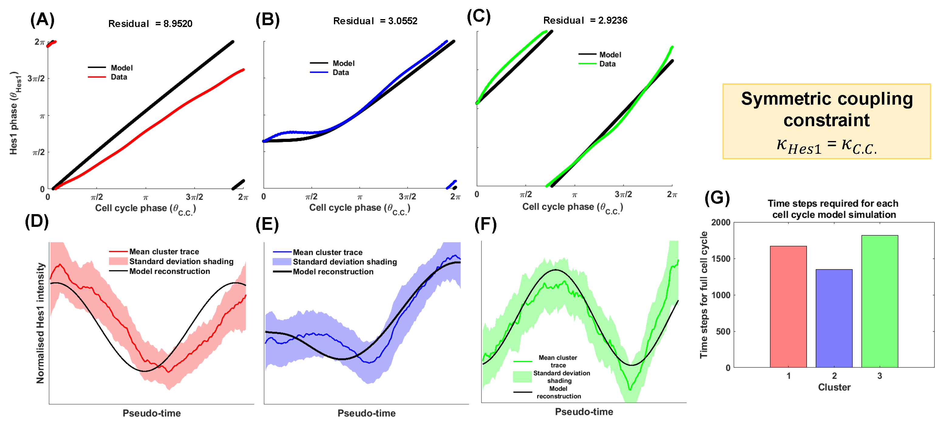
3.2. The Symmetric Interaction Strength Scenario

Let us first assume that the strength of effect that each oscillator has on the other is identical, i.e., κ Hes1 = κ C . C . , we shall call this the symmetric case since the sine function within Equation (5) will mean that any increase in speed by one oscillator will be mirrored by an equivalent decrease in speed by the other and vice-versa. An interesting finding would be if the real-world data can be recapitulated by a simple model with only three parameters (two frequency constants and one coupling constant) compared to four.
Notably, here the cluster 1 trajectory (Figure 5A) is very similar to the corresponding image in the uncoupled case (Figure 4A) and matches the data well. This time, however, the cluster 2 trajectory also performs well in tracking the data (Figure 5B). The Cluster 3 trajectory fits the data better than in the uncoupled case, and this can be seen in the larger upward trend at the end of the cell cycle in Figure 5F than in Figure 4F. The symmetric model is a clear improvement upon the uncoupled case, and this is quantified in the residual values at the top of Figure 5A–C. However, we can see in Figure 5G that this model is insufficient since there exists a discrepancy between cell cycle predictions made by the model and the duration data seen in Figure 1F; comparisons between clusters are not maintained. The symmetric model predicts shorter cell cycles for cluster 2 than cluster 1, a feature that is not present in Figure 1F. This is likely because, for the dynamics to be matched in Figure 5B, then θ Hes1 must slow down, and the symmetry of the system means that θ C . C . must then speed up in an equivalent manner, yielding a faster cell cycle length simulation. Therefore, we can conclude that for our symmetric model, accuracy in either the simulation time or the dynamics must be sacrificed for cluster 2. Thus, the full extent of our data cannot be replicated. This logically leads us to our next step, where we may break the symmetry of our model and consider the asymmetric case where the κ Hes1 = κ C . C . constraint is removed. The results of these simulations are shown below.

3.3. The Unconstrained Interaction Strength Scenario

Figure 6A–F shows that solution trajectories θ Hes1 ( i ) in the asymmetric case also match Θ Hes1 ( i ) , i = 1 , 2 , 3 well, but it is in Figure 6G where a more notable result lies: breaking the symmetry of our system allows for both phase dynamics and cell cycle duration comparisons to mimic that of the data seen in Figure 1. This is an important prediction from our model since we do not originally impose cell cycle lengths into the model, yet the expected lengths are consistent with our observations in [26] when the dynamics are fitted in pseudo-time.
We have found optimal solutions that recapture our data well. However, it may be plausible that a system with even fewer degrees of freedom is sufficient to imitate what we see in Figure 1. Therefore, we also tested (and excluded) the possibility that a one-directional interaction model can explain the data, as displayed in Appendix A. Below, we summarise our results by tabulating residual errors as well as collating the cell cycle length simulations for each constraint case in order to confirm, qualitatively, which of our models works best.

3.4. Asymmetry in Interaction Strength Is Predictive of Elongation in Bcsc Data

Table 1 shows that, overall, the case with the lowest residual error when compared to the data is the one with no constraints upon the coupling strength constants. What is also noticeable is that in Figure 7, the case that matches the data closest is also that of no constraints (modelling strategy 5). We may note that cluster 3’s simulation lengths in the κ Hes1 = 0 case (modelling strategy 4) predict long cluster 3 cell cycles and are promising; however, the cluster 2 simulation lengths are shorter than cluster 1 here, which is not what we see in the data (Figure 1F). We find that by constraining the interaction to be unidirectional, in one case, we have a good fit to dynamics but not to the cell cycle simulations, and in the other case, the opposite is true. Therefore, we determine, overall, that the case where the coupling is allowed to be asymmetric yields the best results, thus we may conclude that bidirectionality is a required feature of our system in order to replicate the data we have. Next, we examine the parameter values κ Hes1 and κ C . C . , which provided the optimal fits and discuss why it might be necessary that they are unconstrained.

3.5. Cluster-Dependent Coupling Strength Points to Gene Expression and Cell Cycle Duration Differences

First, we inspect the cluster 1 case where Hes1 is initially around a peak in oscillation: Figure 8A shows that the distance between the model solution and data is very similar for all pairs of κ Hes1 and κ C . C . , i.e., the data can be explained by a wide parameter region. This suggests that there are no possible combinations of coupling strength parameters that will divert Hes1 from its peak-to-peak behaviour within a cell cycle simulation when beginning with these initial conditions.
Secondly, we note that the initial Hes1 conditions for clusters 2 and 3 are similar in phase value θ Hes1 ( 2 ) ( t 0 ) θ Hes1 ( 3 ) ( t 0 ) < π 2 yet, fascinatingly, require vastly different coupling strength parameters in order to fit the data. The optimal cluster 2 parameters show that a strong effect from the cell cycle onto the Hes1 oscillator and a weak effect in the opposite direction is necessary for the data to be closely replicated. Contrastingly, these effects are required to be weak in both directions for the cluster 3 case, albeit with a slight preference for a greater influence of the Hes1 phase on the cell cycle.
The heatmaps in Figure 8B,C appear to be almost inverted versions of one another; as though they are mutually exclusive cases. This suggests that there is something fundamentally different happening within cells when Hes1 begins a cell cycle before vs. after a trough in an oscillatory wave. Another noteworthy point is that when κ Hes1 > κ C . C . (e.g., the cluster 2 case), the trajectory on the torus diagram (Figure 6B) is initially horizontally slanted. This implies that the effect from θ C . C . onto θ Hes1 is a repressive one, i.e., the cell cycle oscillator is slowing down the Hes1 oscillator. Similarly, we can deduce that only a repressive effect is being felt by the cell cycle oscillator in its progression in the cluster 3 case since the cell cycle predictions are being elongated in Figure 6G; this suggests that θ C . C . is slowing down in its progression. Additionally, it appears to be the lack of effect of the Hes1 oscillator onto the cell cycle oscillator, which explains why we see the cluster 2 cell cycle length predictions from the model being similar to that of cluster 1 in Figure 6G: no elongation/shortening has occurred. Since the equations that make up our model are not overly complicated, we are able to analyse the system Equation (5) with our optimal parameter values to gain mechanistic insight into why we see these results mathematically.

3.6. Mathematical Analysis and Long-Term Behaviour of Our Model

Analysis of the ODE system Equation (5) (see [64]) shows us that there exists a stable and unstable phase-locked trajectory on the torus if
ω Hes1 ω C . C . < κ Hes1 ω Hes1 + κ C . C . ω C . C . .
We may now check to see whether this inequality holds with the parameters discovered in the modelling in this paper. Succinctly, Table 2 shows the parameter values that developed the results from the optimal strategy, as seen in Figure 6.
By plugging the values from Table 2 into the condition of Equation (7), we can analytically show that the trajectories with the coupling parameter values in the cluster 1 and 2 cases will asymptotically approach a stable, periodic phase-locked solution in which both oscillators ( θ Hes1 and θ C . C . ) run at a so-called compromised frequency ω * [64]. However, since the parameters in the cluster 3 case do not meet the condition of Equation(7), and, in fact, the inequality faces the other direction, this means that the trajectory will exhibit a phenomenon known as quasiperiodicity, in which phase-locking between the cell cycle and Hes1 can never occur. Below, we illustrate simulations of long-term solutions to Equation (5) in the square torus diagram with the parameter values from Table 2 to show this visually.
We see in Figure 9A,B that over many cell cycle simulations, the phase space trajectories in both cluster 1 and cluster 2 scenarios will become phase-locked to a solution that is close to the main diagonal, corresponding to cell divisions occurring at a peak indefinitely. This will not happen with the cluster 3 case; Figure 9C shows quasiperiodic behaviour for this solution in which the trajectory will become arbitrarily close to every point on the torus as time tends to infinity. This would mean that cell division are not fixed to any particular Hes1 phase value. The results of this analysis suggest a qualitative difference in the solutions between cluster 3 (the long cell cycle case) and clusters 1 and 2 (the short cell cycle cases), as seen in Figure 9. It is very clear from the data in [26] that cluster 3 cells are particularly interesting due to the long cell cycle durations they possess. Our model predicts these longer cell cycles; the fact that our model now also predicts that phase-locking can not occur in these cells may be a contributing factor to the cell cycle elongation of these cells.
To end this investigation, we are interested to see what happens to solution trajectories when the oscillators maintain the coupling strength interactions but when Hes1 begins at different initial phases.
Figure 10 illustrates that when Hes1 begins at a certain phase, the bidirectional interaction strengths must be specific for that case for the data to be reproduced. For example, inputting the cluster 3 initial conditions into a simulation with the cluster 2 coupling parameters will yield a trajectory that corresponds to a Hes1 wave that is in anti-phase with cluster 1. We know from [26] that Hes1 does not have these specific mitosis to mitosis dynamics. Therefore, we conclude that it is the initial conditions and the specific bidirectional interaction that is required in each case to reproduce the results seen in [26].

4. Discussion

Our results show that the experimentally observed relationship between the expression dynamics of transcription factor (TF) Hes1 and the cell cycle can be described mathematically by a simple, deterministic model of coupled oscillators. Briefly, the experimental results that this work was based on were that, in a Human Breast Cancer cell line, the oscillatory protein expression of the Hes1 TF and the cell cycle fall into three clusters of related dynamics. Namely, one cell cycle from each cluster consists of high-low-high Hes1 dynamics in cluster 1, medium-low-high dynamics in cluster 2 and low-high-low-high dynamics in cluster 3. Cluster 1 cells divide at the peak of the Hes1 wave, which has been described as the preferential in-phase relationship of the majority of the cells, with a concomitant regular 24 h cell cycle length. By contrast, cluster 3 cells divide at the trough (“out-of-phase”); these include cells with significantly longer cell cycles. Cluster 2 cells exhibit an intermediate behaviour, dividing at the downward arm of Hes1 expression and having a 24 h cell cycle length.
Here, we have shown that when the two processes, Hes1 and the cell cycle, are represented only by their phase variables, the parameterised system of nonlinear ODEs from Equation (5) succeeds at generating phase space trajectories. These, in turn, predict the dynamic Hes1 expression behaviour found in the experimental data mentioned above. Furthermore, we have shown here that when the model is parameterised to the time-independent Hes1 data only, the number of time steps required to complete cell cycle simulations mimics the cell cycle duration patterns that are seen in the three clusters in human BCCs.
Our mathematical model shows that both Hes1 dynamics and cell cycle length information taken from real-world data are replicated if, and only if, the following allowances are made: (1) bidirectional coupling is allowed, (2) the symmetry of the system is allowed to be broken such that the coupling strength between cell cycle and Hes1 can differ in each direction and, furthermore, (3) the coupling strength parameter values are not maintained across each cluster case (i.e., they are different between clusters). The first prediction of bidirectional coupling is consistent with our previous experimental data [26]. However, the idea that the interaction strength between the oscillators may differ in either direction and that this happens on a cluster-dependent basis is unexpected and novel. Thus, this work offers a mathematical explanation for the complex outcome of the relationship between Hes1 and the cell cycle [26] and, furthermore, offers some novel parameterisation that will inform future work.
An intriguing product of the simulations is that the parameterisation of the model suggests that neither of the oscillators increases in their speed of progression. In fact, in the cluster 2 and 3 cases, one oscillator will slow down in order for the other to catch up to it. This is evidenced in cluster 2 by a plateau in Hes1 dynamics, yet cell cycle lengths remain similar to that of cluster 1. We may make some thought-provoking hypotheses from these findings: first, Hes1 dynamics cannot induce cell division, but it can delay it. Secondly, the cell cycle machinery can cause Hes1 protein abundance to plateau but not produce quicker oscillations. Future laboratory experimentation will be needed to test these hypotheses. A specific hypothesis to be tested is that of Hes1 being an integral controller, which has been found to be the case in other cell cycle systems such as the Whi5-Cln-cdk1 system [68]. Indeed this would work well with the result found in [26] of a positive correlation between cell cycle duration times and the shape of the Hes1 protein peak and, specifically, the “area under the curve” of Hes1 protein before its first peak was reached.
The benefits of using a simple mathematical model, such as Equation (5), is that it is intuitive, analytically manageable, easy to simulate computationally and yet still offers up surprising and worthwhile results. A more complicated model in the literature, focusing on neural progenitors instead of BCCs, takes into consideration many more interactive molecular species. Interestingly, although Hes1 operates on a much shorter, ultradian periodicity scale [49], it offers a similar conclusion, in part, suggesting that the behaviour of Hes1 is involved in the elongation of the G1-phase and hence the cell cycle. However, the model of [49] differs from ours in that it is unidirectional, meaning that no component of the large model feeds onto Hes1 expression offering no opportunity for Hes1 to be affected by the cell cycle. The interaction terms κ Hes1 and κ C . C . , which we predict to be important here, may relate to the strength by which Hes1 represses cell cycle molecules, such as p21 and cyclin D [49], both of which are known molecular targets of Hes1. In the opposite direction, the cell cycle may be coupled to Hes1 via cell cycle-dependent phosphorylation of the Hes1 protein. Since Hes1 is a Notch signalling target, this could be due to variable Notch signalling during the cell cycle [69].
This is a point at which we may concede that the model in [49] has an advantage over ours as it contains many molecular components and is thus more detailed, allowing for closer inspection of the cell cycle’s inner workings. The ease of parameterisation of our functional model, on the other hand, is an advantage since the dynamics are uncomplicated to study. Going forward, this model could be easily adapted or modified to include more biological realism, e.g., including the addition of some external force acting upon one or both of the oscillators or offering some uncertainty quantification. Should our current hypothesis of the importance of changing bidirectionality be experimentally refuted, then it may be that the data is reproducible with the addition of the concept of a phase delay as is discussed in [70,71]. This may also be true with the introduction of oscillatory concepts such as dead zones (see [72]); this may be particularly fruitful since it is apparent that Hes1 is not responding to the cell cycle progression at the beginning of the cluster 2 trajectory in Figure 6. Further experimentation would be required to justify the implementation of these ideas.
This paper has been focused solely on Hes1’s relationship with one full cell cycle and has ignored the existence of previous or subsequent generations of cells. In future work, it would be interesting to see whether the coupling strength between the oscillators is capable of changing between generations. Changes over time within a cell lineage may align well with the fact that BCSCs are known to be plastic in nature, and interconversion between stem cell subtypes is known to occur [29,73]. The allocation of cells into Hes1 dynamic clusters also shows conversion between generations. Multigenerational analysis of Hes1 dynamics/cell cycle length will also be needed to elucidate the hypothesis of a “phase-skipping“ in Hes1, which may occur when the cell divides [26]. The concept of a phase-skipping event (also described as a hlphase-slip in [63]) of an oscillator due to stochasticity has been studied in [57], where it is stated that the “phenomenon occurs when a fluctuation in the non-deterministic elements exceeds the stability domain of the attractor”. Such an event with the mammalian circadian oscillator has been found to be linked to DNA damage in [74,75]. Phase skipping may also take place here since the periodicity of Hes1 studied here is circadian-like [26], and it would be interesting to examine the connection to DNA damage, especially since the data have been collected in MCF-7 cells, which are a model for breast cancer. In a cancer model, phase skipping and the associated elongation of the cell cycle may have important ramifications for the development and progression of the disease and could be a topic for future experimental and theoretical work on multigenerational gene expression of Hes1.
In summary, we have demonstrated in this theory paper that complex biological data, such as gene expression dynamics, can be modelled effectively using a straight-forward concept and very few core assumptions. By considering phases rather than protein abundances over time, we have been able to view the complicated landscape of genetic cell biology in a different light and strip back potentially superfluous detail to uncover key factors in the relationship between Hes1 and the cell cycle. This will allow us to propose new hypotheses (e.g., plasticity in cell cycle/Hes1 coupling strength between generations, phase-skipping of the Hes1 oscillator at a cell division) and promote exciting future work endeavours that would have otherwise been hidden.

Author Contributions

Conceptualization, A.R.; methodology, A.R.; software, A.R.; validation, all authors; formal analysis, A.R.; investigation, A.R.; resources, N.P.; data curation, A.R. and N.S.; writing—original draft preparation, A.R.; writing—review and editing, A.R. and N.P.; visualization, A.R.; supervision, N.P.; project administration, N.P.; funding acquisition, N.P. All authors have read and agreed to the published version of the manuscript.

Funding

The work was funded by a Wellcome Trust Senior Research Fellowship to N.P. (106185/Z/14/Z). and a Wellcome Trust Investigator Award to N.P. (224394/Z/21/Z).

Institutional Review Board Statement

Not applicable.

Informed Consent Statement

Not applicable.

Data Availability Statement

MATLAB code used for computing model simulations can be found in a repository through the following link: https://github.com/AndyRowntree/MATLAB-code-for-paper-Rowntree-et.-al.- (accesed on 27 May 2022).

Acknowledgments

We thank Nikos Kavallaris for the kind invitation to submit to this journal and the Papalopulu lab members for their helpful comments and support of this work. The work was sponsored by the Wellcome Trust Grant 106185/Z/14/Z (to N.P.).

Conflicts of Interest

The authors declare no conflict of interest.

Appendix A. Unidirectional Interaction Constraints

In Figure A1 we see the trajectories in the square torus diagrams following the data well yet the cell cycle simulation times are all nearly identical, which does not match the data. In Figure A2 we see that with no external influence on f Hes1 , the trajectory in the cluster 2 case is not able to plateau to match the corresponding data trajectory. However, the cell cycle length simulations are more similar to the data.
Figure A1. Results of the solutions to the model Equation (5) with the constraint κ C . C . = 0 when θ Hes1 ( i ) is optimised to the data vector Θ Hes1 ( i ) , i = 1 , 2 , 3 , frequency parameters are set as ω Hes1 = 24 1 and ω C . C . = 27 1 . (AC) Square torus diagram trajectories of solutions θ Hes1 ( i ) , i = 1, 2, 3 superimposed over data trajectories from Figure 2B. (DF) Psedo-time plots of rebuilt Hes1 dynamics found via cos θ Hes1 ( i ) , i = 1 , 2 , 3 superimpsoed over mean traces from Figure 2A. In (AF), the black lines denote the model results, coloured lines denote the data (red: cluster 1, blue: cluster 2 and green: cluster 3), and in (DF), the shaded areas denote the standard deviations of the data. (G) Bar chart of cell cycle duration predictions from the simulation for each cluster case.
Mathematics 10 02323 g0a1
Figure A2. Results of the solutions to the model Equation (5) with the constraint κ Hes1 = 0 when θ Hes1 ( i ) is optimised to the data vector Θ Hes1 ( i ) , i = 1 , 2 , 3 , frequency parameters are set as ω Hes1 = 24 1 and ω C . C . = 27 1 . (AC) Square torus diagram trajectories of solutions θ Hes1 ( i ) , i = 1, 2, 3 superimposed over data trajectories from Figure 2B. (DF) Psedo-time plots of rebuilt Hes1 dynamics found via cos θ Hes1 ( i ) , i = 1 , 2 , 3 superimposed over mean traces from Figure 2A. In (AF), the black lines denote the model results, coloured lines denote the data (red: cluster 1, blue: cluster 2 and green: cluster 3), and in (DF), the shaded areas denote the standard deviations of the data. (G) Bar chart of cell cycle duration predictions from the simulation for each cluster case.
Mathematics 10 02323 g0a2

References

  1. Purvis, J.E.; Karhohs, K.W.; Mock, C.; Batchelor, E.; Loewer, A.; Lahav, G. p53 dynamics control cell fate. Science 2012, 336, 1440–1444. [Google Scholar] [CrossRef] [Green Version]
  2. Imayoshi, I.; Isomura, A.; Harima, Y.; Kawaguchi, K.; Kori, H.; Miyachi, H.; Kageyama, R. Oscillatory control of factors determining multipotency and fate in mouse neural progenitors. Science 2013, 342, 1203–1208. [Google Scholar] [CrossRef] [PubMed] [Green Version]
  3. Manning, C.S.; Biga, V.; Boyd, J.; Kursawe, J.; Ymisson, B.; Spiller, D.G.; Papalopulu, N. Quantitative single-cell live imaging links HES5 dynamics with cell-state and fate in murine neurogenesis. Nat. Commun. 2019, 10, 2835. [Google Scholar] [CrossRef] [PubMed] [Green Version]
  4. Longo, D.; Hasty, J. Dynamics of single-cell gene expression. Mol. Syst. Biol. 2006, 2, 64. [Google Scholar] [CrossRef] [Green Version]
  5. Sonnen, K.F.; Janda, C.Y. Signalling dynamics in embryonic development. Biochem. J. 2021, 478, 4045–4070. [Google Scholar] [CrossRef]
  6. Purvis, J.E.; Lahav, G. Encoding and decoding cellular information through signaling dynamics. Cells 2013, 152, 945–956. [Google Scholar] [CrossRef] [PubMed] [Green Version]
  7. Martin, E.; Sung, M.H. Challenges of Decoding Transcription Factor Dynamics in Terms of Gene Regulation. Cells 2018, 7, 132. [Google Scholar] [CrossRef] [Green Version]
  8. Behar, M.; Dohlman, H.G.; Elston, T.C. Kinetic insulation as an effective mechanism for achieving pathway specificity in intracellular signaling networks. Proc. Natl. Acad. Sci. USA 2007, 104, 16146–16151. [Google Scholar] [CrossRef] [PubMed] [Green Version]
  9. Roberts, K.; Alberts, B.; Johnson, A.; Walter, P.; Hunt, T. Molecular Biology of the Cell, 6th ed.; Garland Science: New York, NY, USA, 2015; pp. 963–967. [Google Scholar]
  10. Tyson, J.J.; Csikasz-Nagy, A.; Novak, B. The dynamics of cell cycle regulation. Bioessays 2002, 24, 1095–1109. [Google Scholar] [CrossRef] [Green Version]
  11. Qu, Z.; MacLellan, W.R.; Weiss, J.N. Dynamics of the cell cycle: Checkpoints, sizers, and timers. Biophys. J. 2003, 85, 3600–3611. [Google Scholar] [CrossRef] [Green Version]
  12. Dalton, S. Linking the cell cycle to cell fate decisions. Trends Cell Biol. 2015, 25, 592–600. [Google Scholar] [CrossRef] [PubMed] [Green Version]
  13. Pauklin, S.; Vallier, L. The cell-cycle state of stem cells determines cell fate propensity. Cell 2013, 155, 135–147. [Google Scholar] [CrossRef] [PubMed] [Green Version]
  14. Roccio, M.; Schmitter, D.; Knobloch, M.; Okawa, Y.; Sage, D.; Lutolf, M.P. Predicting stem cell fate changes by differential cell cycle progression patterns. Development 2013, 140, 459–470. [Google Scholar] [CrossRef] [Green Version]
  15. de Lichtenberg, K.H.; Seymour, P.A.; Jørgensen, M.C.; Kim, Y.H.; Grapin-Botton, A.; Magnuson, M.A.; Serup, P. Notch controls multiple pancreatic cell fate regulators through direct Hes1-mediated repression. BioRxiv 2019, 336305. [Google Scholar]
  16. Kageyama, R.; Ohtsuka, T.; Tomita, K. The bHLH gene Hes1 regulates differentiation of multiple cell types. Mol. Cells 2000, 10, 1–7. [Google Scholar] [CrossRef]
  17. Kageyama, R.; Ohtsuka, T.; Kobayashi, T. Roles of Hes genes in neural development. Dev. Growth Differ. 2008, 50, S97–S103. [Google Scholar] [CrossRef]
  18. Isomura, A.; Kageyama, R. Ultradian oscillations and pulses: Coordinating cellular responses and cell fate decisions. Development 2014, 141, 3627–3636. [Google Scholar] [CrossRef] [PubMed] [Green Version]
  19. Marinopoulou, E.; Biga, V.; Sabherwal, N.; Miller, A.; Desai, J.; Adamson, A.D.; Papalopulu, N. HES1 protein oscillations are necessary for neural stem cells to exit from quiescence. Iscience 2021, 24, 103198. [Google Scholar] [CrossRef]
  20. Noda, N.; Honma, S.; Ohmiya, Y. Hes1 is required for contact inhibition of cell proliferation in 3T3-L1 preadipocytes. Genes Cells 2011, 16, 704–713. [Google Scholar] [CrossRef]
  21. Murata, K.; Hattori, M.; Hirai, N.; Shinozuka, Y.; Hirata, H.; Kageyama, R.; Minato, N. Hes1 directly controls cell proliferation through the transcriptional repression of p27Kip1. Mol. Cell. Biol. 2005, 25, 4262–4271. [Google Scholar] [CrossRef] [Green Version]
  22. Ochi, S.; Imaizumi, Y.; Shimojo, H.; Miyachi, H.; Kageyama, R. Oscillatory expression of Hes1 regulates cell proliferation and neuronal differentiation in the embryonic brain. Development 2020, 147, dev182204. [Google Scholar] [CrossRef]
  23. Cenciarelli, C.; Marei, H.E.; Zonfrillo, M.; Casalbore, P.; Felsani, A.; Giannetti, S.; Mangiola, A. The interference of Notch1 target Hes1 affects cell growth, differentiation and invasiveness of glioblastoma stem cells through modulation of multiple oncogenic targets. Oncotarget 2017, 8, 17873. [Google Scholar] [CrossRef] [PubMed] [Green Version]
  24. Sang, L.; Roberts, J.M.; Coller, H.A. Hijacking HES1: How tumors co-opt the anti-differentiation strategies of quiescent cells. Trends Mol. Med. 2010, 16, 17–26. [Google Scholar] [CrossRef] [PubMed] [Green Version]
  25. Liu, Z.H.; Dai, X.M.; Du, B. Hes1: A Key Role in Stemness, Metastasis and Multidrug Resistance. Cancer Biol. Ther. 2015, 16, 353–359. [Google Scholar] [CrossRef] [PubMed] [Green Version]
  26. Sabherwal, N.; Rowntree, A.; Marinopoulou, E.; Pettini, T.; Hourihane, S.; Thomas, R.; Papalopulu, N. Differential phase register of Hes1 oscillations with mitoses underlies cell-cycle heterogeneity in ER+ breast cancer cells. Proc. Natl. Acad. Sci. USA 2021, 118, e2113527118. [Google Scholar] [CrossRef] [PubMed]
  27. Comşa, Ş.; Cimpean, A.M.; Raica, M. The story of MCF-7 breast cancer cell line: 40 years of experience in research. Anticancer Res. 2015, 35, 3147–3154. [Google Scholar]
  28. Lee, A.V.; Oesterreich, S.; Davidson, N.E. MCF-7 cells—Changing the course of breast cancer research and care for 45 years. J. Natl. Cancer Inst. 2015, 107, djv073. [Google Scholar] [CrossRef] [Green Version]
  29. Liu, S.; Cong, Y.; Wang, D.; Sun, Y.; Deng, L.; Liu, Y.; Wicha, M.S. Breast cancer stem cells transition between epithelial and mesenchymal states reflective of their normal counterparts. Stem Cell Rep. 2014, 2, 78–91. [Google Scholar] [CrossRef]
  30. Hirata, H.; Yoshiura, S.; Ohtsuka, T.; Bessho, Y.; Harada, T.; Yoshikawa, K.; Kageyama, R. Oscillatory expression of the bHLH factor Hes1 regulated by a negative feedback loop. Science 2002, 298, 840–843. [Google Scholar] [CrossRef] [Green Version]
  31. Monk, N.A. Oscillatory expression of Hes1, p53, and NF-kB driven by transcriptional time delays. Curr. Biol. 2003, 13, 1409–1413. [Google Scholar] [CrossRef] [Green Version]
  32. Momiji, H.; Monk, N.A. Dissecting the dynamics of the Hes1 genetic oscillator. J. Theor. Biol. 2008, 254, 784–798. [Google Scholar] [CrossRef]
  33. Ay, A.; Arnosti, D.N. Mathematical modeling of gene expression: A guide for the perplexed biologist. Crit. Rev. Biochem. Mol. Biol. 2011, 46, 137–151. [Google Scholar] [CrossRef] [Green Version]
  34. Robert, P. Mathematical models of gene expression. Probab. Surv. 2019, 16, 277–332. [Google Scholar] [CrossRef]
  35. Smolen, P.; Baxter, D.A.; Byrne, J.H. Mathematical modeling of gene networks. Neuron 2000, 26, 567–580. [Google Scholar] [CrossRef] [Green Version]
  36. Goodfellow, M.; Phillips, N.E.; Manning, C.; Galla, T.; Papalopulu, N. microRNA input into a neural ultradian oscillator controls emergence and timing of alternative cell states. Nat. Commun. 2014, 5, 3399. [Google Scholar] [CrossRef] [PubMed] [Green Version]
  37. Phillips, N.E.; Manning, C.S.; Pettini, T.; Biga, V.; Marinopoulou, E.; Stanley, P.; Papalopulu, N. Stochasticity in the miR-9/Hes1 oscillatory network can account for clonal heterogeneity in the timing of differentiation. eLife 2016, 5, e16118. [Google Scholar] [CrossRef] [PubMed] [Green Version]
  38. Barrio, M.; Burrage, K.; Leier, A.; Tian, T. Oscillatory regulation of Hes1: Discrete stochastic delay modelling and simulation. PLoS Comput. Biol. 2006, 2, e117. [Google Scholar] [CrossRef] [Green Version]
  39. Pfeuty, B. Multistability and transitions between spatiotemporal patterns through versatile Notch-Hes signaling. J. Theor. Biol. 2022, 539, 111060. [Google Scholar] [CrossRef]
  40. Bertuzzi, A.; Gandolfi, A.; Giovenco, M.A. Mathematical models of the cell cycle with a view to tumor studies. Math. Biosci. 1981, 53, 159–188. [Google Scholar] [CrossRef]
  41. Basse, B.; Baguley, B.C.; Marshall, E.S.; Joseph, W.R.; van Brunt, B.; Wake, G.; Wall, D.J. A mathematical model for analysis of the cell cycle in cell lines derived from human tumors. J. Math. Biol. 2003, 47, 295–312. [Google Scholar] [CrossRef]
  42. Sible, J.C.; Tyson, J.J. Mathematical modeling as a tool for investigating cell cycle control networks. Methods 2007, 41, 238–247. [Google Scholar] [CrossRef] [PubMed] [Green Version]
  43. Gérard, C.; Goldbeter, A. Temporal self-organization of the cyclin/Cdk network driving the mammalian cell cycle. Proc. Natl. Acad. Sci. USA 2009, 106, 21643–21648. [Google Scholar] [CrossRef] [PubMed] [Green Version]
  44. Weis, M.C.; Avva, J.; Jacobberger, J.W.; Sreenath, S.N. A data-driven, mathematical model of mammalian cell cycle regulation. PloS ONE 2014, 9, e97130. [Google Scholar] [CrossRef] [PubMed] [Green Version]
  45. Tyson, J.J.; Novák, B. Models in biology: Lessons from modeling regulation of the eukaryotic cell cycle. BMC Biol. 2015, 13, 46. [Google Scholar] [CrossRef] [Green Version]
  46. Shao, Q.; Cortes, M.G.; Trinh, J.T.; Guan, J.; Balázsi, G.; Zeng, L. Coupling of DNA replication and negative feedback controls gene expression for cell-fate decisions. Iscience 2018, 6, 1–12. [Google Scholar] [CrossRef] [Green Version]
  47. Tyson, J.J.; Baumann, W.T.; Chen, C.; Verdugo, A.; Tavassoly, I.; Wang, Y.; Clarke, R. Dynamic modelling of oestrogen signalling and cell fate in breast cancer cells. Nat. Rev. Cancer 2011, 11, 523–532. [Google Scholar] [CrossRef] [PubMed]
  48. Pfeuty, B.; David-Pfeuty, T.; Kaneko, K. Underlying principles of cell fate determination during G1 phase of the mammalian cell cycle. Cell Cycle 2008, 7, 3246–3257. [Google Scholar] [CrossRef]
  49. Pfeuty, B.A. A computational model for the coordination of neural progenitor self-renewal and differentiation through Hes1 dynamics. Development 2015, 142, 3. [Google Scholar] [CrossRef] [Green Version]
  50. Strogatz, S.H. The Mathematical Structure of the Human Sleep-Wake Cycle; Springer: New York, NY, USA, 1986; Volume 69. [Google Scholar]
  51. Strogatz, S.H. Human sleep and circadian rhythms: A simple model based on two coupled oscillators. J. Math. Biol. 1987, 25, 327–347. [Google Scholar] [CrossRef]
  52. Burton, J.; Manning, C.S.; Rattray, M.; Papalopulu, N.; Kursawe, J. Inferring kinetic parameters of oscillatory gene regulation from single cell time-series data. J. R. Soc. Interface 2021, 18, 20210393. [Google Scholar] [CrossRef]
  53. Paulsson, J. Models of stochastic gene expression. Phys. Life Rev. 2005, 2, 157–175. [Google Scholar] [CrossRef]
  54. Fan, M.; Kuwahara, H.; Wang, X.; Wang, S.; Gao, X. Parameter estimation methods for gene circuit modeling from time-series mRNA data: A comparative study. Brief. Bioinform. 2015, 16, 987–999. [Google Scholar] [CrossRef] [PubMed] [Green Version]
  55. Gérard, C.; Goldbeter, A. Entrainment of the mammalian cell cycle by the circadian clock: Modeling two coupled cellular rhythms. PLoS Comput. Biol. 2012, 8, e1002516. [Google Scholar] [CrossRef] [PubMed]
  56. Yang, Q.; Pando, B.F.; Dong, G.; Golden, S.S.; van Oudenaarden, A. Circadian gating of the cell cycle revealed in single cyanobacterial cells. Science 2010, 327, 1522–1526. [Google Scholar] [CrossRef] [PubMed] [Green Version]
  57. Feillet, C.; Krusche, P.; Tamanini, F.; Janssens, R.C.; Downey, M.J.; Martin, P.; Rand, D.A. Phase locking and multiple oscillating attractors for the coupled mammalian clock and cell cycle. Proc. Natl. Acad. Sci. USA 2014, 111, 9828–9833. [Google Scholar] [CrossRef] [PubMed] [Green Version]
  58. Droin, C.; Paquet, E.R.; Naef, F. Low-dimensional dynamics of two coupled biological oscillators. Nat. Phys. 2019, 15, 1086–1094. [Google Scholar] [CrossRef]
  59. Tyson, J.J.; Novák, B. Irreversible transitions, bistability and checkpoint controls in the eukaryotic cell cycle: A systems-level understanding. In Handbook of Systems Biology; Elsevier: San Diego, CA, USA, 2012; pp. 265–285. [Google Scholar]
  60. Pomerening, J.R.; Kim, S.Y.; Ferrell, J.E., Jr. Systems-level dissection of the cell-cycle oscillator: Bypassing positive feedback produces damped oscillations. Cell 2005, 122, 565–578. [Google Scholar] [CrossRef] [Green Version]
  61. Ferrell, J.E., Jr.; Pomerening, J.R.; Kim, S.Y.; Trunnell, N.B.; Xiong, W.; Huang, C.Y.F.; Machleder, E.M. Simple, realistic models of complex biological processes: Positive feedback and bistability in a cell fate switch and a cell cycle oscillator. FEBS Lett. 2009, 583, 3999–4005. [Google Scholar] [CrossRef] [Green Version]
  62. Tyson, J.J.; Novak, B. Temporal organization of the cell cycle. Curr. Biol. 2008, 18, R759–R768. [Google Scholar] [CrossRef] [Green Version]
  63. Pikovsky, A.; Rosenblum, M.; Kurths, J. Synchronization: A Universal Concept in Nonlinear Science; Cambridge University Press: Cambridge, UK, 2001. [Google Scholar]
  64. Strogatz, S.H. Nonlinear Dynamics and Chaos: With Applications to Physics, Biology, Chemistry, and Engineering, 2nd ed.; Westview press: Boulder, CO, USA, 2015; pp. 276–281. [Google Scholar]
  65. Kuramoto, Y. Self-entrainment of a population of coupled non-linear oscillators International symposium on mathematical problems in theoretical physics. Lect. Notes Phys. 1975, 30, 420. [Google Scholar]
  66. Morelli, L.G.; Ares, S.; Herrgen, L.; Schröter, C.; Jülicher, F.; Oates, A.C. Delayed coupling theory of vertebrate segmentation. HFSP J. 2009, 3, 55–66. [Google Scholar] [CrossRef] [PubMed] [Green Version]
  67. Biga, V.; Hawley, J.; Soto, X.; Johns, E.; Han, D.; Bennett, H.; Papalopulu, N. A dynamic, spatially periodic, micro-pattern of HES5 underlies neurogenesis in the mouse spinal cord. Mol. Syst. Biol. 2021, 17, e9902. [Google Scholar] [CrossRef] [PubMed]
  68. Liu, X.; Wang, X.; Yang, X.; Liu, S.; Jiang, L.; Qu, Y.; Tang, C. Reliable cell cycle commitment in budding yeast is ensured by signal integration. eLife 2015, 4, e03977. [Google Scholar] [CrossRef] [PubMed]
  69. Carrieri, F.A.; Murray, P.J.; Ditsova, D.; Ferris, M.A.; Davies, P.; Dale, J.K. CDK 1 and CDK 2 regulate NICD 1 turnover and the periodicity of the segmentation clock. EMBO Rep. 2019, 20, e46436. [Google Scholar] [CrossRef]
  70. Woo, J.H.; Honey, C.J.; Moon, J.Y. Phase and amplitude dynamics of coupled oscillator systems on complex networks. Chaos Interdiscip. J. Nonlinear Sci. 2020, 30, 121102. [Google Scholar] [CrossRef] [PubMed]
  71. Pietras, B.; Daffertshofer, A. Network dynamics of coupled oscillators and phase reduction techniques. Phys. Rep. 2019, 819, 1–105. [Google Scholar] [CrossRef]
  72. Ashwin, P.; Bick, C.; Poignard, C. Dead zones and phase reduction of coupled oscillators. Chaos Interdiscip. J. Nonlinear Sci. 2021, 31, 093132. [Google Scholar] [CrossRef]
  73. Gupta, P.B.; Fillmore, C.M.; Jiang, G.; Shapira, S.D.; Tao, K.; Kuperwasser, C.; Lander, E.S. Stochastic state transitions give rise to phenotypic equilibrium in populations of cancer cells. Cell 2011, 146, 633–644. [Google Scholar] [CrossRef] [PubMed] [Green Version]
  74. Oklejewicz, M.; Destici, E.; Tamanini, F.; Hut, R.A.; Janssens, R.; van der Horst, G.T. Phase resetting of the mammalian circadian clock by DNA damage. Curr. Biol. 2008, 18, 286–291. [Google Scholar] [CrossRef] [Green Version]
  75. Hong, C.I.; Zámborszky, J.; Csikász-Nagy, A. Minimum criteria for DNA damage-induced phase advances in circadian rhythms. PLoS Comput. Biol. 2009, 5, e1000384. [Google Scholar] [CrossRef] [Green Version]
Figure 1. Graphs and schematics representing the results in [26]. (A) Schematic illustrating that cell division at a peak in Hes1 yields regular and consistent cell cycle durations (top panel) whereas division at a trough gives rise to longer cell cycles (middle panel). Schematic of cyclins (cell cycle proteins) that rise and fall in abundance once every cell cycle (bottom panel). (BD): There exist three distinct mitosis to mitosis dynamic behaviours of normalized (z-scored) Hes1 expression: Cluster 1 with high-low-high, Cluster 2 with medium-low-high and Cluster 3 with low-high-low-high dynamics (red, blue, green lines, respectively, shading is ± one standard deviation). (E) The momentary position within the oscillation (i.e., the phase that we define in Section 2) at the beginning of the cell cycle of each cell (total n = 164) is plotted as a polar histogram and separated by cluster classification. Means are marked by radial lines. (F) Bar chart of mean cell cycle duration of breast cancer cells per cluster. The cells whose Hes1 expression dynamics are classified as Cluster 3 show significantly (p < 0.0001) longer cell cycles than those in Clusters 1 or 2.
Mathematics 10 02323 g001
Figure 2. Developing the phase progression data. (A) Mean traces of all three clustered, normalised (z-scored) Hes1 traces in pseudo-time. (B) A uniformly spaced cell cycle oscillator vector Θ C . C . [ 0 , 2 π ) on the x-axis plotted against the Hes1 oscillator phase reconstruction Θ Hes1 of traces from (A) found via application of the Hilbert transform forming phase space trajectories on a square torus diagram. (C) Alternative view of phase progression between our data vectors Θ Hes1 and Θ C . C . . Both oscillators are represented as points on a circle (coloured dots are the Hes1 and black dots are the cell cycle oscillators), at five snapshotted times within the pseudo-timed cell cycle.
Mathematics 10 02323 g002
Figure 3. Schematic illustrating our method of developing model simulations with an arbitrary example trajectory.
Mathematics 10 02323 g003
Figure 4. Results of the solutions to model Equation (5) with the constraint κ Hes1 = κ C . C . = 0 when θ Hes1 ( i ) is optimised to the data vector Θ Hes1 ( i ) , i = 1 , 2 , 3 , the frequency parameters are set as ω Hes1 = 24 1 and ω C . C . = 27 1 . (AC) Square torus diagram trajectories of solutions θ Hes1 ( i ) , i = 1, 2, 3 superimposed over data trajectories from Figure 2B. (DF) Pseudo-time plots of rebuilt Hes1 dynamics found via cos θ Hes1 ( i ) , i = 1, 2, 3 superimposed over mean traces from Figure 2A. In (AF), the black lines denote the model results, coloured lines denote the data (red: cluster 1, blue: cluster 2 and green: cluster 3) and in (DF) the shaded areas denote the standard deviations of the data. (G) Bar chart of cell cycle duration predictions from the simulation for each cluster case.
Mathematics 10 02323 g004
Figure 5. Results of the solutions to model (5) with the constraint κ Hes1 = κ C . C . when θ Hes1 ( i ) is optimised to the data vector Θ Hes1 ( i ) , i = 1 , 2 , 3 , frequency parameters are set as ω Hes1 = 24 1 and ω C . C . = 27 1 . (AC) Square torus diagram trajectories of solutions θ Hes1 ( i ) , i = 1, 2, 3 superimposed over data trajectories from Figure 2B. (DF) Pseudo-time plots of rebuilt Hes1 dynamics found via cos θ Hes1 ( i ) , i = 1 , 2 , 3 superimposed over mean traces from Figure 2A. In (AF), the black lines denote the model results, coloured lines denote the data (red: cluster 1, blue: cluster 2 and green: cluster 3), and in (DF), the shaded areas denote the standard deviations of the data. (G) Bar chart of cell cycle duration predictions from the simulation for each cluster case.
Mathematics 10 02323 g005
Figure 6. Results of the solutions to model (5) with no parameter constraints when θ Hes1 ( i ) is optimised to the data vector Θ Hes1 ( i ) , i = 1 , 2 , 3 , frequency parameters are set as ω Hes1 = 24 1 and ω C . C . = 27 1 . (AC) Square torus diagram trajectories of solutions θ Hes1 ( i ) , i = 1, 2, 3 superimposed over data trajectories from Figure 2B. (DF) Pseudo-time plots of rebuilt Hes1 dynamics found via cos θ Hes1 ( i ) , i = 1, 2, 3 superimposed over mean traces from Figure 2A. In (AF), the black lines denote the model results, coloured lines denote the data (red: cluster 1, blue: cluster 2 and green: cluster 3), and in (DF), the shaded areas denote the standard deviations of the data. (G) Bar chart of cell cycle duration predictions from the simulation for each cluster case.
Mathematics 10 02323 g006
Figure 7. Bar chart summarising cell cycle simulation times for each parameter constraint case. Taken from (F) in Figure 1 and (G) in Figure 4, Figure 5 and Figure 6, Figure A1 and Figure A2. Bar charts have been normalised by dividing all three by the cluster 1 simulation time value for each constraint. Strategy 5 has been highlighted since it most closely matches the “data”.
Mathematics 10 02323 g007
Figure 8. Heatmaps of two-dimensional κ C . C . × κ Hes1 parameter space with the colour representing the residual value (Euclidean distance) between solution vector θ Hes1 ( i ) and data vector Θ Hes1 ( i ) where i = 1 , 2 , 3 in panels (A–C) respectively, in the case with no parameter constraints. The black x marks the point in this space where the residual is the lowest for each cluster, i.e., the coupling strength parameter values that yielded the best fit to the data and thus those used to produce the results in Figure 6.
Mathematics 10 02323 g008
Figure 9. (AC) Long-term solutions of Equation (5) with optimal parameter values found in Figure 8 for clusters 1, 2 and 3, respectively. (D) Two-dimensional κ C . C . × κ Hes1 parameter space with optimal parameter values found in Figure 8 for clusters 1, 2 and 3 plotted as a red, blue and green x, respectively. The yellow region represents parameters where the condition of Equation (7) is met and when trajectories will asymptotically reach a stable phase-locked solution. The blue region represents the region where Equation (7) is not met, and quasiperiodicity will occur.
Mathematics 10 02323 g009
Figure 10. Torus diagram trajectories for one simulation of Equation (5) at uniformly spaced θ Hes1 ( t 0 ) initial conditions with optimal parameters for cluster 1 in panel (A), cluster 2 in panel (B) and cluster 3 in panel (C), as stated in Table 2. Red, blue and green trajectories in panels (AC) here are the same as the black trajectories in Figure 6A–C, respectively.
Mathematics 10 02323 g010
Table 1. Table of residual comparisons for each modelling strategy 1 to 5. Values are the minimised R values found by fitting the pseudo-timed model solution θ Hes1 ( i ) to Θ Hes1 ( i ) for i = 1 , 2 , 3 within the given parameter constraints. Highlighted in cyan is the strategy with the lowest summed residuals across clusters.
Modelling StrategyCoupling Strength Parameter ConstraintCluster 1Cluster 2Cluster 3Sum
1 κ Hes1 = 0 , κ C . C . = 0 12.119923.52066.811842.4523
2 κ Hes1 = κ C . C . 8.95203.05522.923614.9308
3 κ C . C . = 0 9.92291.78943.077414.7897
4 κ Hes1 = 0 8.83407.37532.875719.085
5Optimal (no constraints)8.83521.79672.870213.5021
Table 2. Table summarizing the optimal κ Hes1 and κ C . C . values for the model Equation (5) for each cluster case.
Cluster123
Initial Hes1 phase (1 d.p.)6.12.03.4
κ Hes1 00.860.01
κ C . C . 0.9900.13
ω Hes1 0.04170.04170.0417
ω C . C . 0.03700.03700.0370
Condition (7) met?YesYesNo
Publisher’s Note: MDPI stays neutral with regard to jurisdictional claims in published maps and institutional affiliations.

