Developed Gorilla Troops Technique for Optimal Power Flow Problem in Electrical Power Systems

 ,
,  ,
,  , and
, and
Abstract
:1. Introduction
- The designed GTOT is exploited to reduce different target functions for minimizing the fuel costs, power losses, and pollutant emissions related to EPSs and applied on the IEEE standard 30 bus and practical WD.
- Multi-dimension operations with two or three objectives are developed in this work.
- The developed GTOT outperforms a number of current approaches, including CST, GWT, ISHT, NBT, and SST.
- Statistical analyses and stability assessments are developed in this work to demonstrate the capability of the proposed GTOT in handling the OPFP with different sizes and objective functions.
- The simulation results of related techniques in the literature are compared with the developed GTOT to demonstrate the robustness and solution quality of GTOT.
- Substantial consistency is accompanied by the proposed GTOT for handling the OPFP in EPSs.
2. Gorilla Troops Optimization Technique
2.1. Exploration Phase
2.2. Exploitation Phase
3. Problem Formulation
3.1. Objectives
3.2. System Constraints
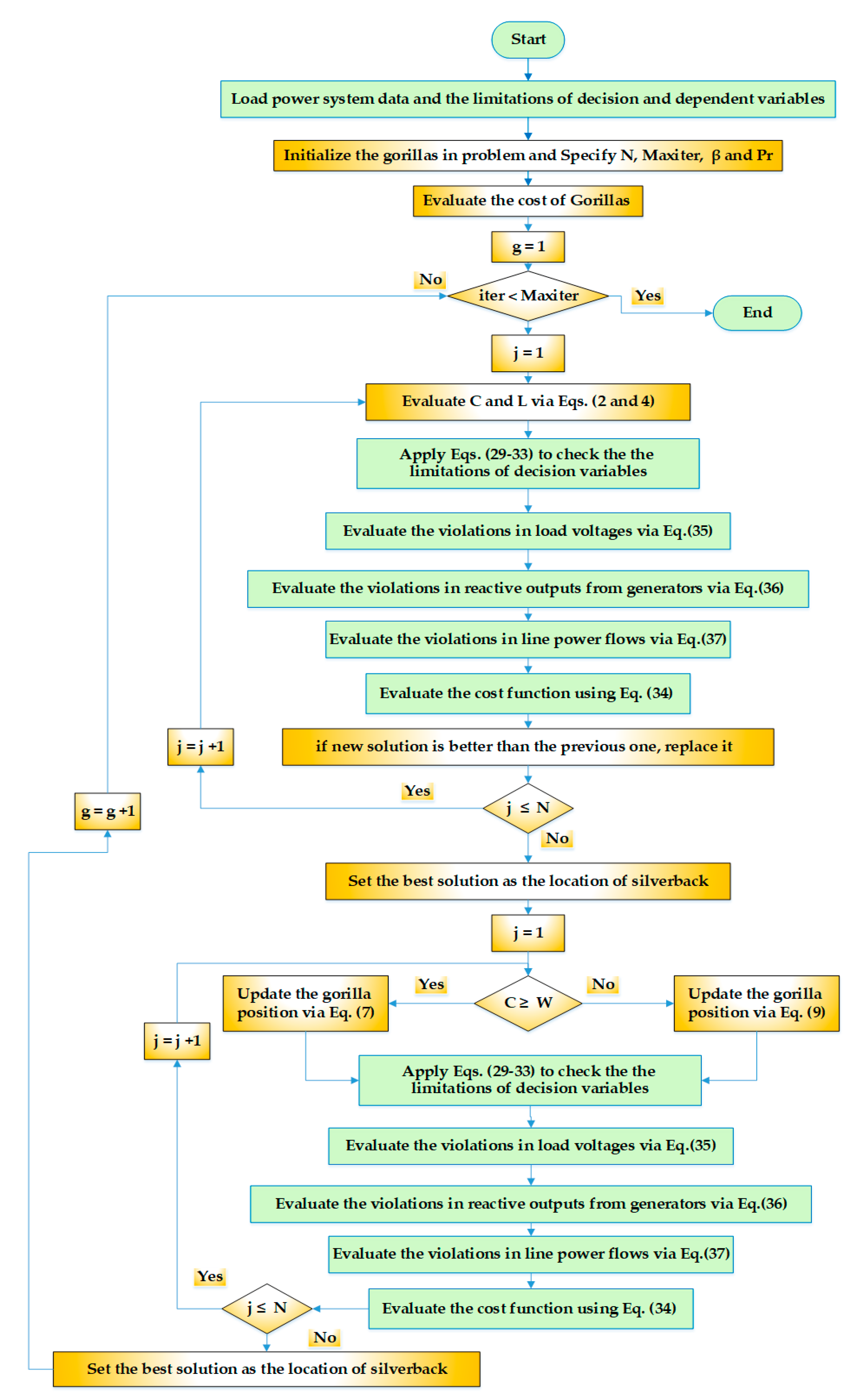
4. Developed Solution-Based GTOT for OPFP in EPSs
4.1. Improvement of GTOT for Incorporating Operational Limitations of Independent Variables
4.2. Improvement of GTOT for Incorporating Operational Limitations of Dependent Variables
5. Simulation Results
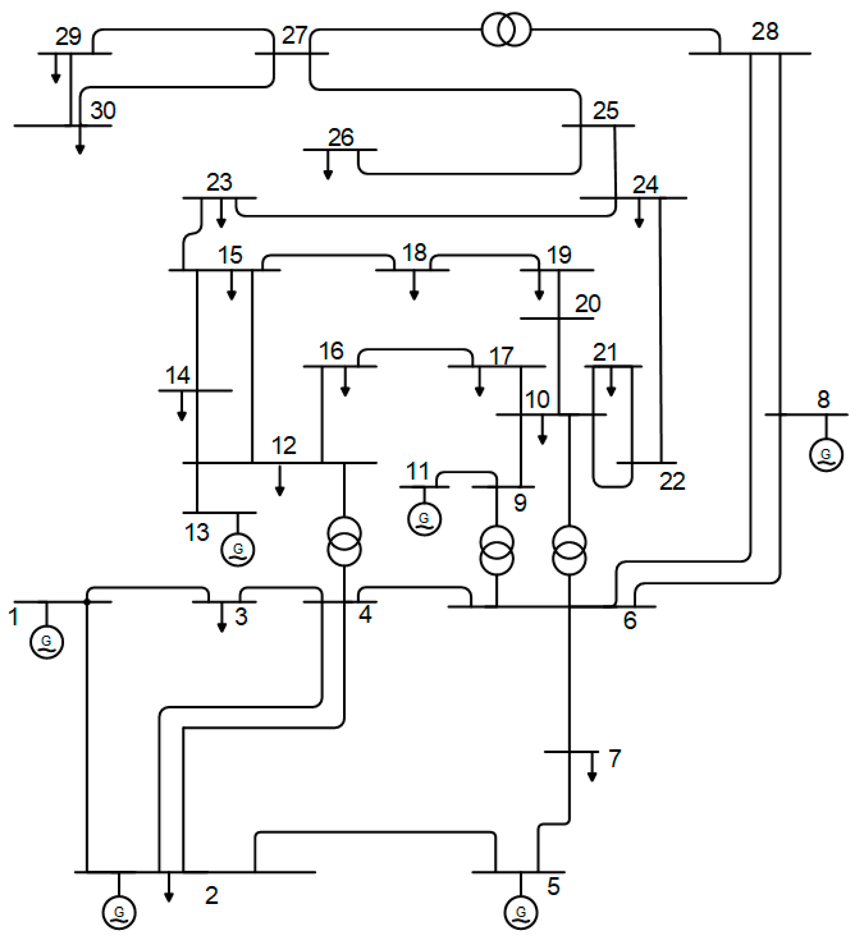
5.1. Results of the First EPS
- Scenario 1: OJ1 minimization of FGCs described in Equation (16);
- Scenario 2: OJ2 minimization of FGCSs described in Equation (17);
- Scenario 3: OJ3 minimization of PE described in Equation (18);
- Scenario 4: OJ4 minimization of OPL described in Equation (19);
- Scenario 5: Merging OJ1 and OJ3 as a multi-objective function;
- Scenario 6: Merging OJ1, OJ3, and OJ4 as a multi-objective function.
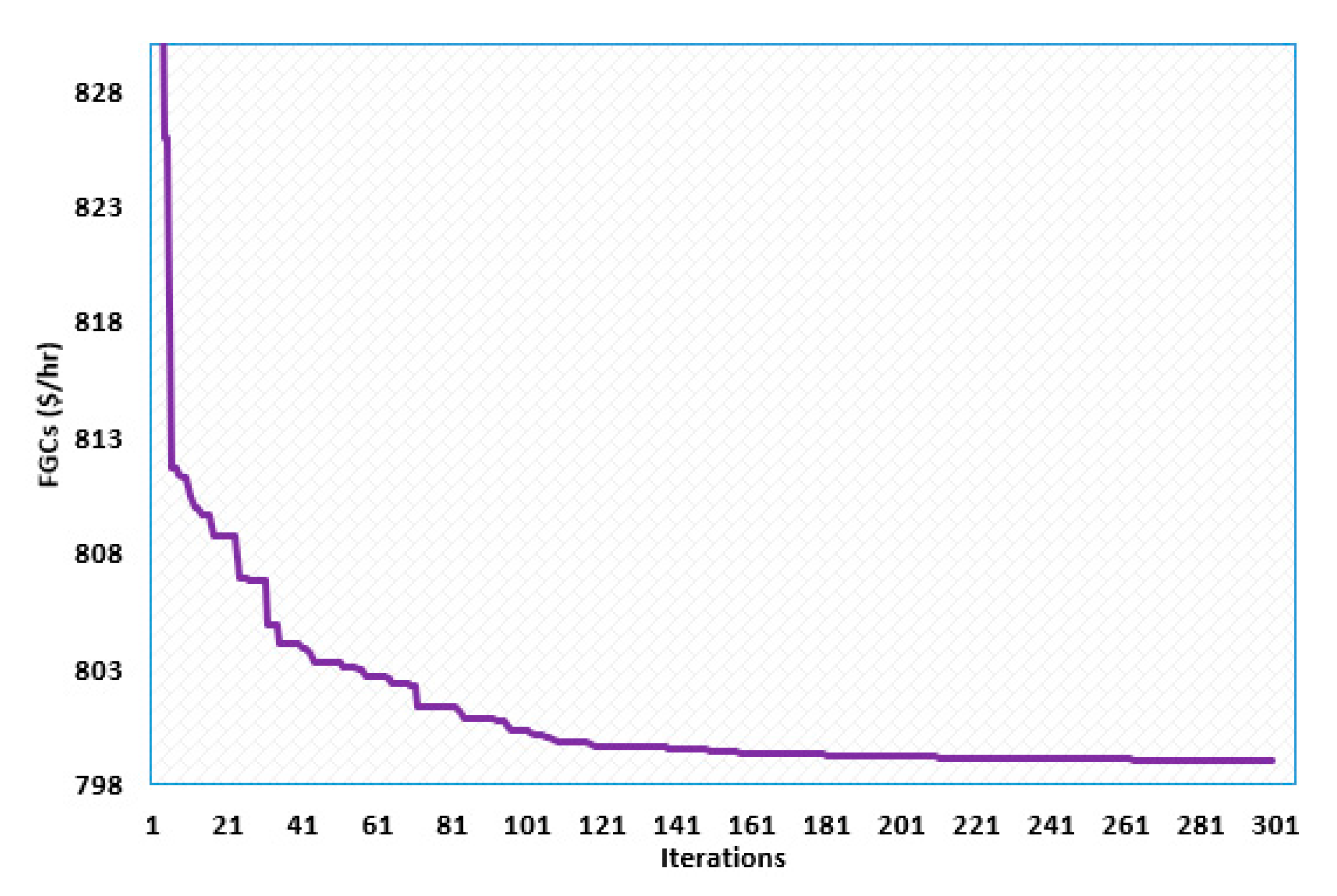
5.1.1. Scenario 1
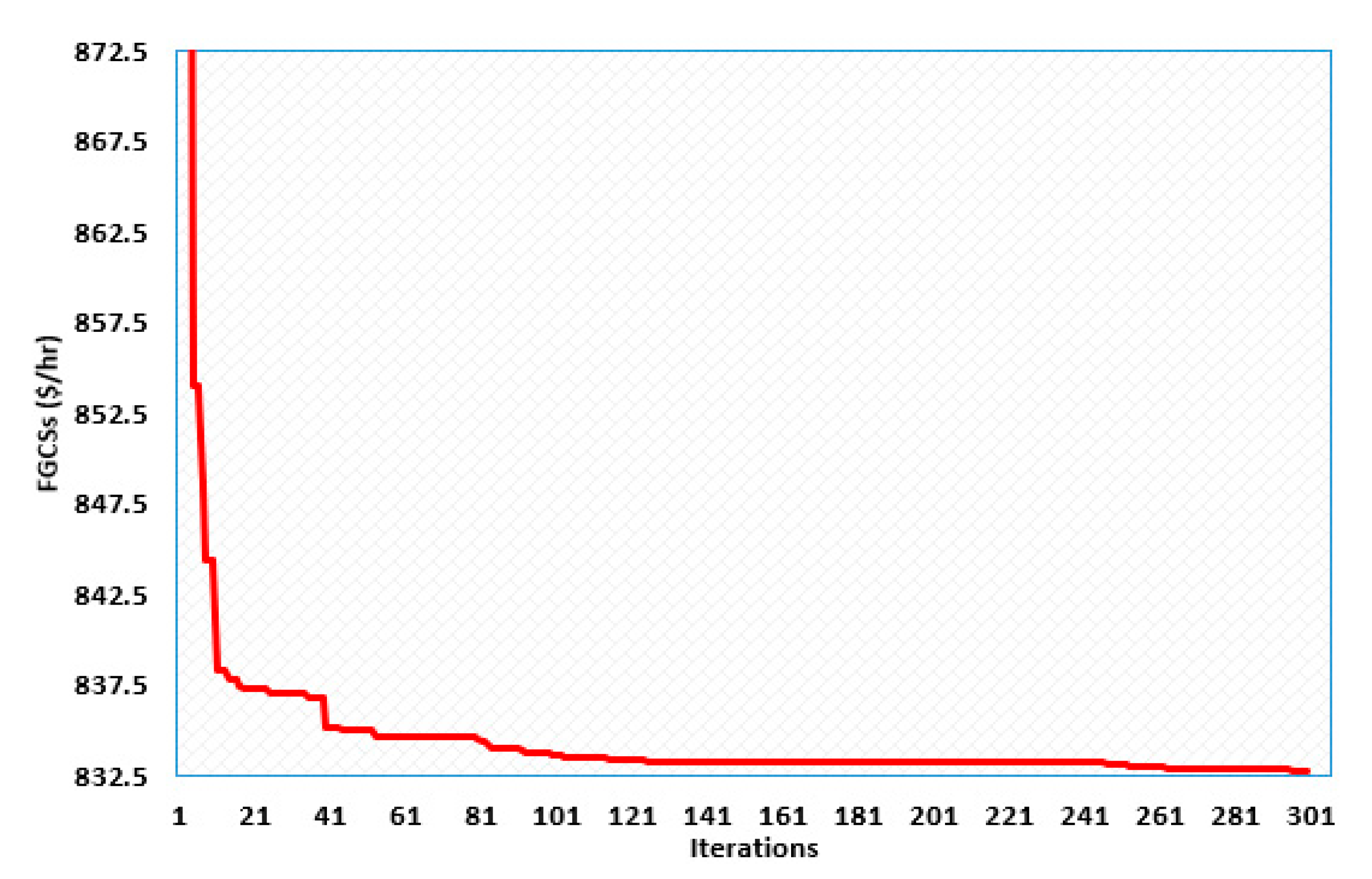
5.1.2. Scenario 2
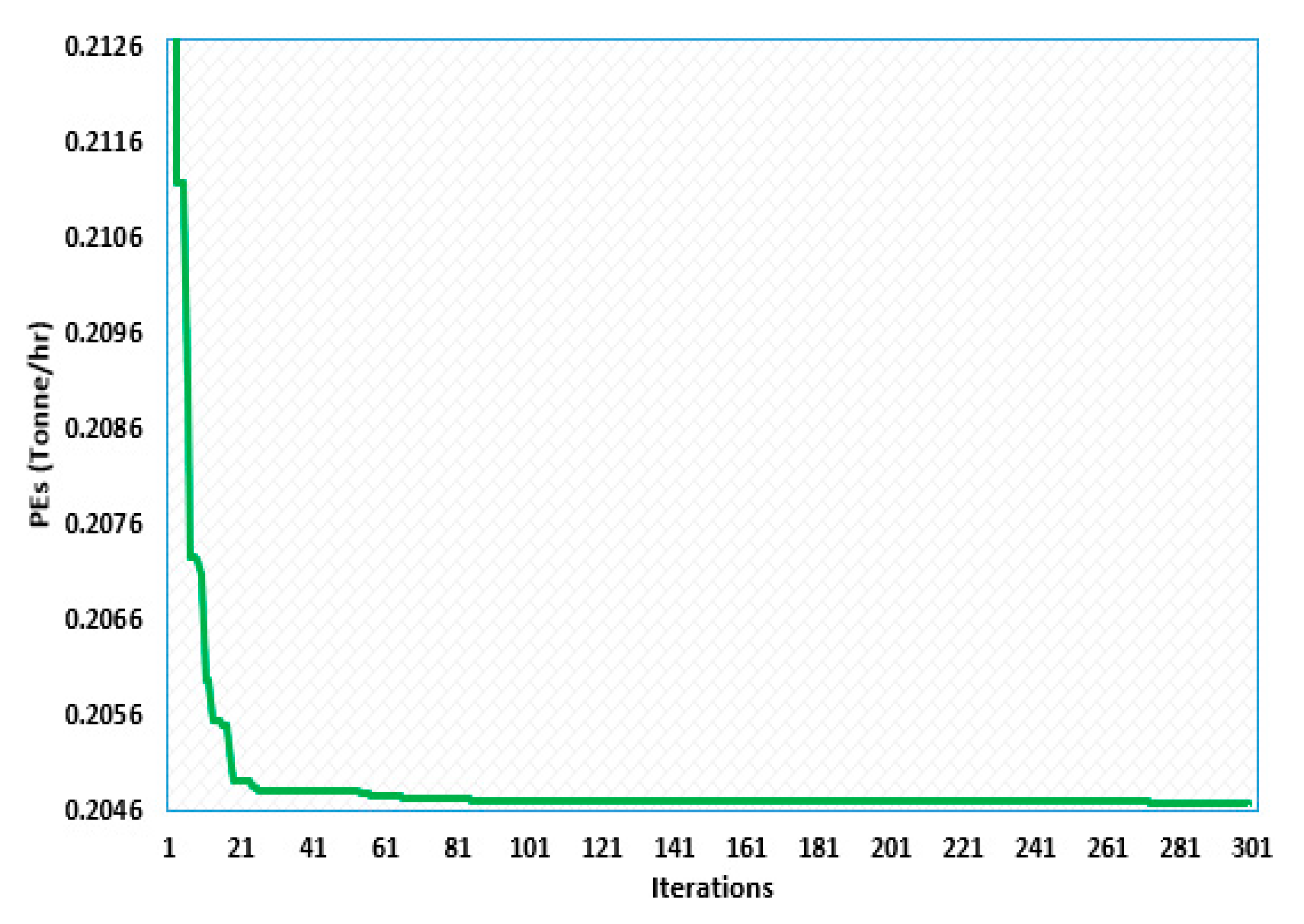
5.1.3. Scenario 3
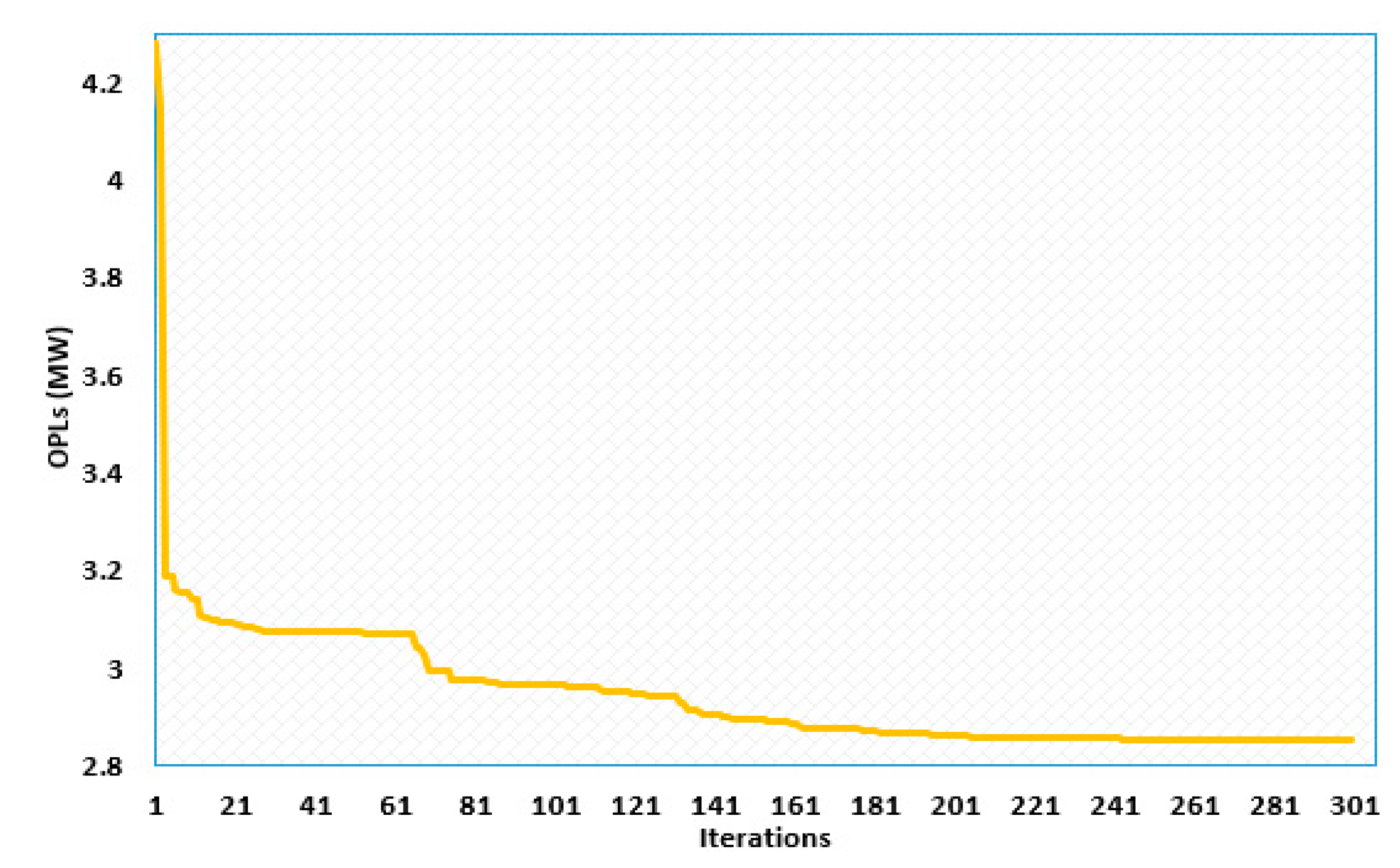
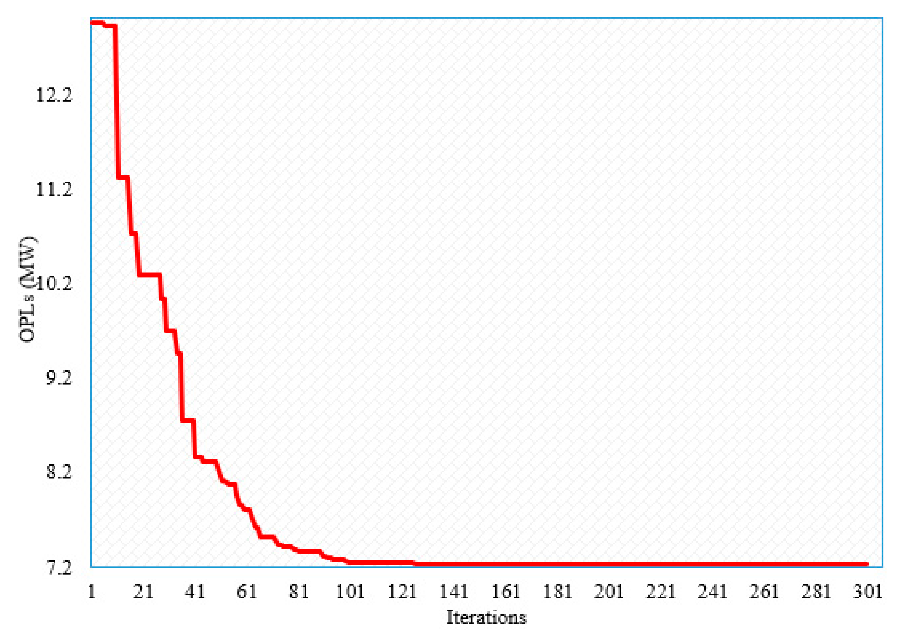
5.1.4. Scenario 4
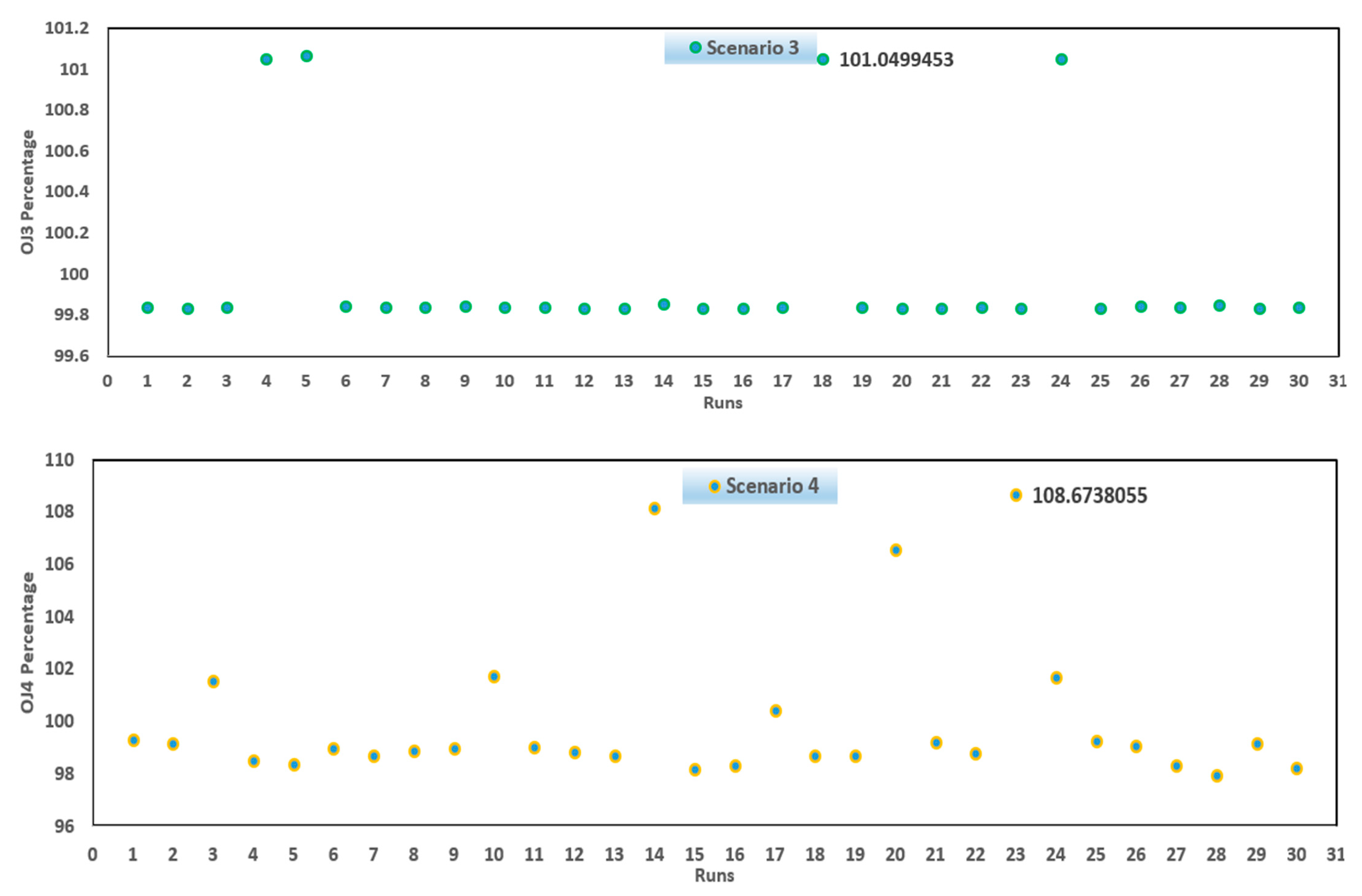
5.1.5. Stability Assessment of the Developed GTOT for the First EPS
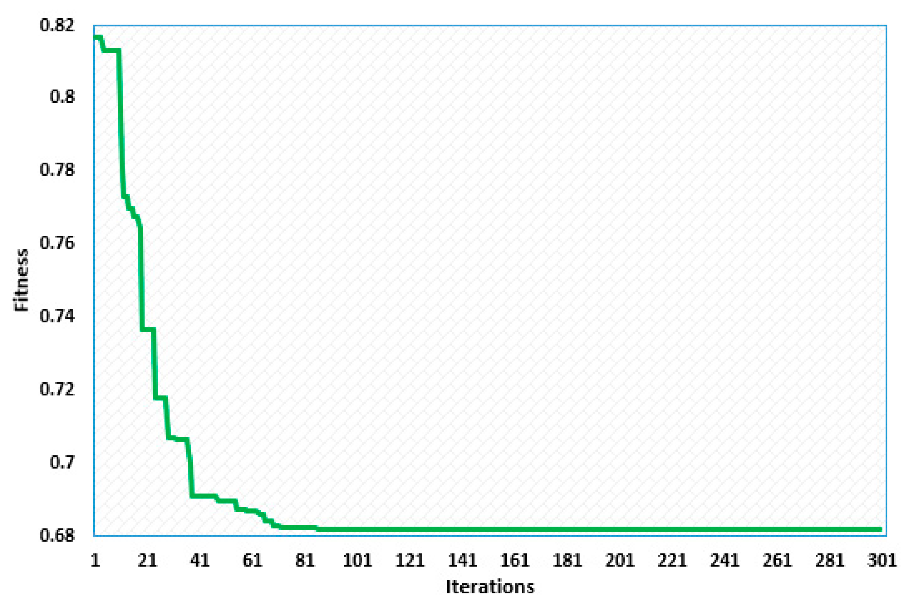
5.1.6. Scenario 5 and Scenario 6
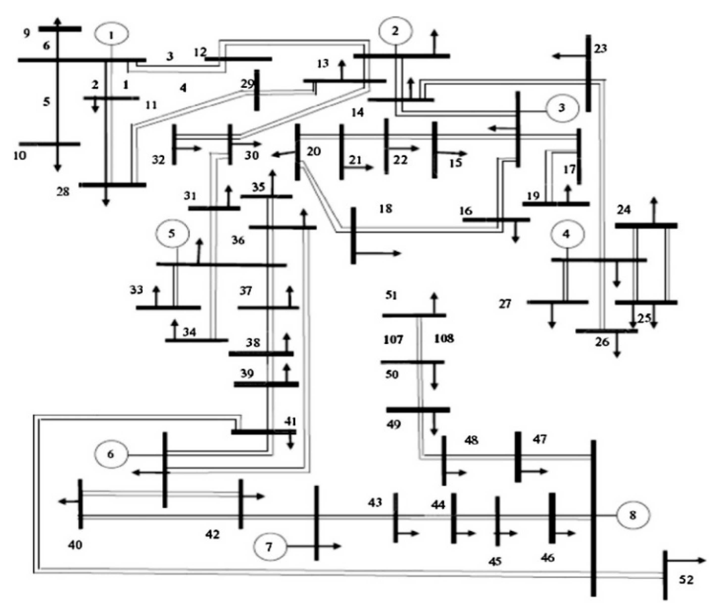
5.2. Results of the Second EPS
- Scenario 7: OJ1 minimization described in Equation (16);
- Scenario 8: OJ4 minimization described in Equation (19);
- Scenario 9: Merging OJ1 and OJ4 as a multi-objective function.
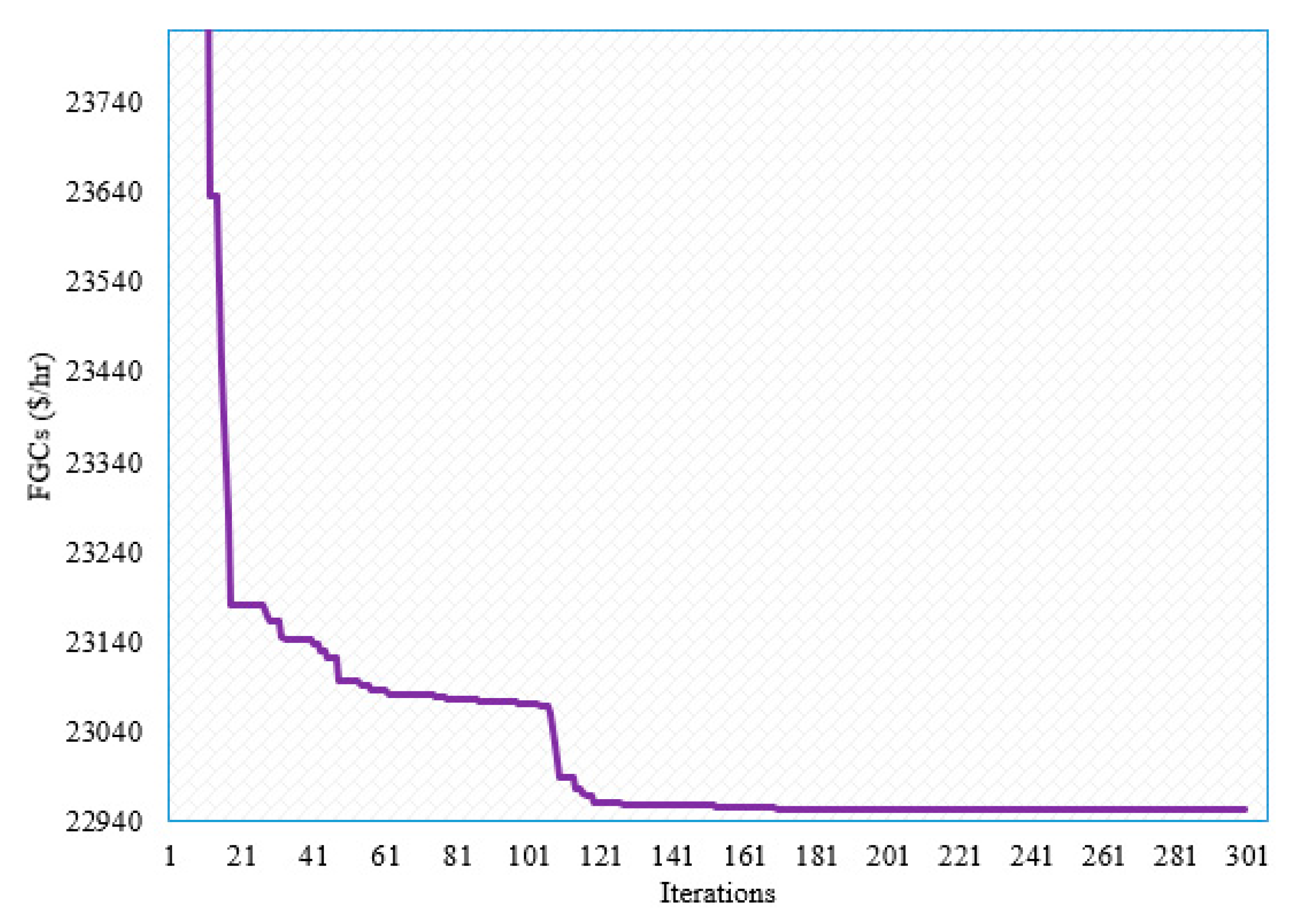
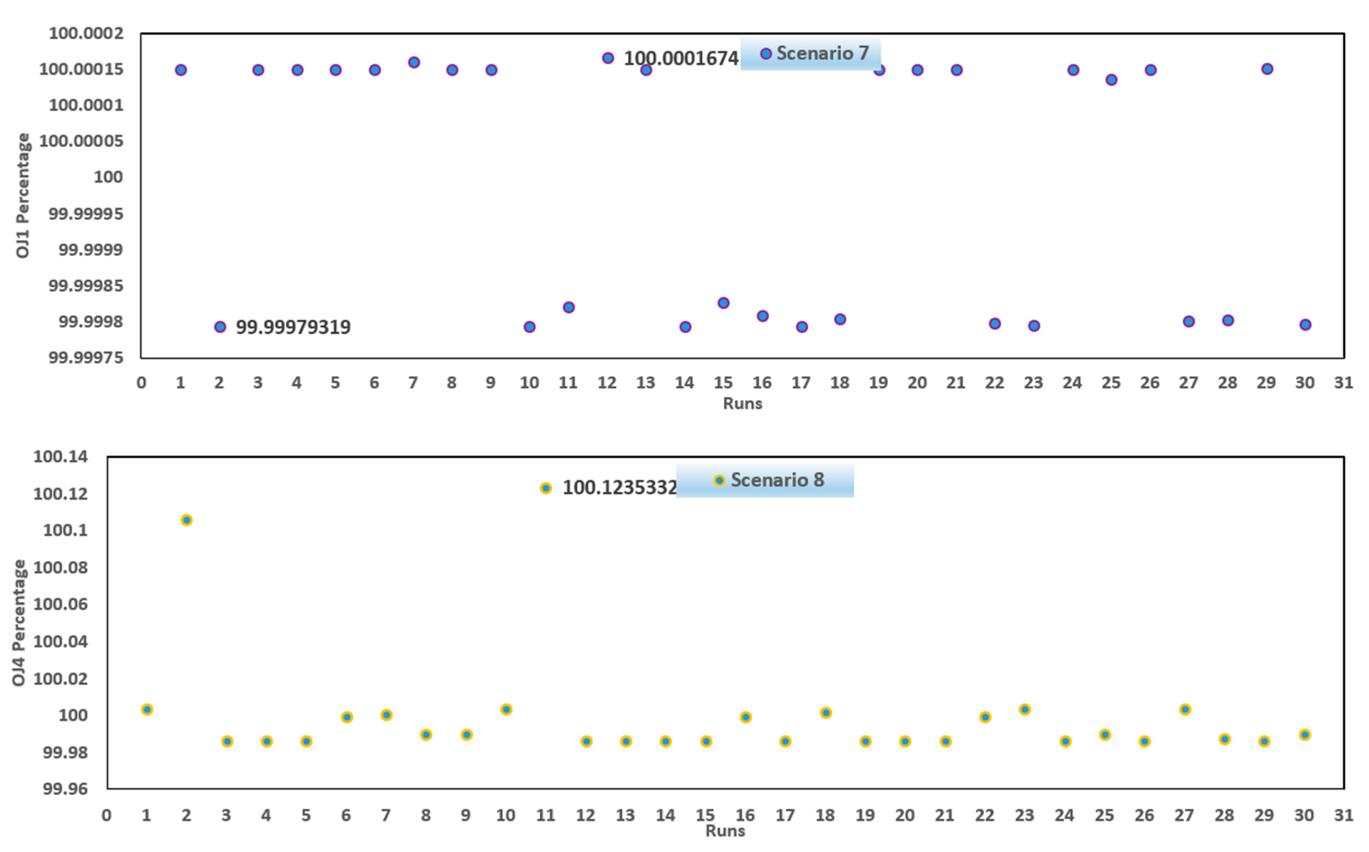
5.2.1. Scenario 7
5.2.2. Scenario 8
5.2.3. Stability Assessment of the GTOT for the Second EPS
5.2.4. Scenario 9
6. Conclusions
- Multi-dimension objectives combining two and three objectives for both systems are developed in this work.
- Their percentages of reduction for the single objectives are reached (11.406%, 7.67%, 14.39%, 51.09%, 8.54%, and 61.95%) for the six single objective scenarios in comparison to the initial circumstance.
- The GTOT is employed in different evaluations and statistical analyses with many modern methods such as GWT, CST, SST, NBT, and ISHT.
- The developed GTOT always has the ability to find a close percentage to 100% where its average is near to its minimum for both EPSs.
- When developed GTOT compared to other similar approaches in the literature, the simulated results demonstrate the designed GTOT’s solution validity and stability.
- The developed GTOT derives considerable stability for all scenarios.
Author Contributions
Funding
Informed Consent Statement
Data Availability Statement
Conflicts of Interest
List of Acronyms
| AGT | Adaptive GT |
| ARBT | Adaptive real biogeography-based technique |
| AGST | Adaptive group search technique |
| BBO | Biogeography-based optimization |
| BHBT | Black-hole-based technique |
| CBOA | Colliding bodies optimization algorithm |
| COA | Coyote optimization algorithm |
| CSSO | Chaotic salp swarm optimizer |
| CST | Crow search technique |
| DE | Differential evolution |
| DHST | Differential harmony search technique |
| EMM | Electromagnetism-like mechanism |
| EPSs | Electrical power systems |
| EMRFT | Enhanced manta ray foraging technique |
| EMSA | Emended moth swarm algorithm |
| FGCs | Fuel generation costs |
| FGCSs | FGC with sinusoids |
| GA | Genetic algorithm |
| GTOT | Gorilla troops optimization technique |
| GT | Grasshopper technique |
| GWT | Grey wolf technique |
| HGWODE | Hybridization of GWT and DE |
| ICT | Imperialist competitive technique |
| IEOT | Improved electromagnetism-like technique |
| IMFT | Improved moth-flame technique |
| INSGA-III | Improved non-dominated sorting genetic algorithm |
| ISHT | Improved spotted-hyena technique |
| ISST | Improved social spider technique |
| IADE | Adaptive differential evolution |
| JFST | Jellyfish search technique |
| KHT | Krill herd technique |
| MCST | Modified crow search technique |
| NBT | Novel bat technique |
| MRFT | Manta-ray foraging technique |
| MST | Moth swarm technique |
| OPFP | Optimal power flow problem |
| OPL | Overall power loss |
| PE | Produced emissions |
| PSO | Particle swarm optimization |
| QCMFT | Quantum computing and moth flame technique |
| SAO | Simulated annealing optimization |
| SOST | Symbiotic organisms search technique |
| SST | Salp swarm technique |
| TLT | Teaching-learning technique |
| WCEMFT | Combination of water cycle with moth flame technique |
| WD | West delta |
| WD-EPS | West Delta-EPS |
List of Variables
| A | Level of violence in a fight |
| Xr | The current group position of gorilla |
| LL | Variables’ minimum bound |
| X(g) | Vector of gorilla location in the g iteration |
| GX(g + 1) | Vector of gorilla location in the g + 1 iteration |
| rand, rd1, rd2, rd3 | Random values ranging from 0 to 1 |
| Pr | Migrating coefficient |
| GXr | Candidate group position of gorilla |
| UL | Variables’ maximum bound |
| Iter | Present iteration number |
| MaxIter | Maximum iteration number |
| rd4 | Random value inside the bound [0:1] |
| l | Random values between −1 and 1 |
| X(g) | Vector of gorilla location |
| Q | Force of impact |
| rd5 | Random value within bound [0:1] |
| β | Pre-optimization value |
| E | Violence efficacy |
| Vg1, Vg2, …, VgNg) | Voltages of the generators |
| Tap1, Tap2, … TapNt | Tap changer settings |
| Nt | Number of on-load tap changers |
| Qg1, Qg2, …, QgNg | Generator reactive power outputs |
| Pg1, Pg2, …, PgNg | Generators’ real power output |
| OJ | Investigated vector of several m targets |
| OJ1 | Costs of fuel generation in dollars per hour |
| Pgk | Real power output in megawatts of generator |
| OJ2 | Costs of fuel generation with sinusoids |
| θ | Phase angle |
| Gmn | Conductance of a line between buses m and n |
| QL | Power consumption in its reactive components |
| Gjk | Mutual conductance of line between bus j and k |
| VLj | Load voltage at bus j |
| OJj | Each objective function |
| NRA | Newton–Raphson approach |
| Pen3 | Penalty coefficient for any violation in line flow |
| Ng | Number of on-load generators |
| Nq | Number of on-load reactive power sources, |
| SF1, …, SFNF | Transmission flow limits |
| Z | Random values between [−c:c] |
| Xsilverback | The best solution which is the silverback |
| N | Population of gorillas |
| A | Level of violence in a fight |
| VL1, …, VLNPQ | Load bus voltage magnitudes |
| NPQ | The number of load buses, |
| x | Independent variables |
| y | Dependent variables |
| m | Vector of several targets |
| k; Ck, Bk, and Ak | Cost factors of generator k |
| NF | Number of transmission lines |
| Qc1, Qc2, …, QcNq | Reactive power injections of switching capacitors |
| Lowest limitation of generator k | |
| Ek and Fk | Generator k’s sinusoid cost factors |
| OJ3 | Produced ton/hr emissions from the power plants |
| γk, βk, αk, ξk, and λk | Emission factors of generator k |
| Nb | Number of buses |
| V | Voltage |
| PL | Power consumption in its active components |
| Bjk | Mutual susceptance of a line between bus j and k |
| Sfl | Power flow via line |
| Pen1 | Penalty coefficient for violation in load voltage |
| Pen2 | Penalty coefficient for violation in reactive power output from generators |
| IndOJk | Mean value |
References
- Trivedi, I.N.; Jangir, P.; Parmar, S.A.; Jangir, N. Optimal Power Flow with Voltage Stability Improvement and Loss Reduction in Power System Using Moth-Flame Optimizer. Neural Comput. Appl. 2018, 30, 1889–1904. [Google Scholar] [CrossRef]
- Buch, H.; Trivedi, I.N.; Jangir, P. Moth Flame Optimization to Solve Optimal Power Flow with Non-Parametric Statistical Evaluation Validation. Cogent Eng. 2017, 4, 1286731. [Google Scholar] [CrossRef]
- Attia, A.F.; El Sehiemy, R.A.; Hasanien, H.M. Optimal Power Flow Solution in Power Systems Using a Novel Sine-Cosine Algorithm. Int. J. Electr. Power Energy Syst. 2018, 99, 331–343. [Google Scholar] [CrossRef]
- Montoya, O.D. A Convex OPF Approximation for Selecting the Best Candidate Nodes for Optimal Location of Power Sources on DC Resistive Networks. Eng. Sci. Technol. Int. J. 2020, 23, 527–533. [Google Scholar] [CrossRef]
- Bai, X.; Wei, H. A Semidefinite Programming Method with Graph Partitioning Technique for Optimal Power Flow Problems. Int. J. Electr. Power Energy Syst. 2011, 33, 1309–1314. [Google Scholar] [CrossRef]
- Dommel, H.W.; Tinney, W.F. Optimal Power Flow Solutions. IEEE Trans. Power Appar. Syst. 1968, PAS-87, 1866–1876. [Google Scholar] [CrossRef]
- Crisan, O.; Mohtadi, M.A. Efficient Identification of Binding Inequality Constraints in the Optimal Power Flow Newton Approach. IEE Proc. C Gener. Transm. Distrib. 1992, 139, 365–370. [Google Scholar] [CrossRef]
- Mota-Palomino, R.; Quintana, V.H. Sparse Reactive Power Scheduling by a Penalty Function-Linear Programming Technique. IEEE Trans. Power Syst. 1986, 1, 31–39. [Google Scholar] [CrossRef]
- Granelli, G.P.; Montagna, M. Security-Constrained Economic Dispatch Using Dual Quadratic Programming. Electr. Power Syst. Res. 2000, 56, 71–80. [Google Scholar] [CrossRef]
- Burchett, R.C.; Happ, H.H.; Vierath, D.R. Quadratically Convergent Optimal Power Flow. IEEE Trans. Power Appar. Syst. 1984, PAS-103, 3267–3275. [Google Scholar] [CrossRef]
- El-Sehiemy, R.A.; El Ela, A.A.A.; Shaheen, A. A Multi-Objective Fuzzy-Based Procedure for Reactive Power-Based Preventive Emergency Strategy. Int. J. Eng. Res. Afr. 2015, 13, 91–102. [Google Scholar] [CrossRef]
- Rahli, M.; Pirotte, P. Optimal Load Flow Using Sequential Unconstrained Minimization Technique (SUMT) Method under Power Transmission Losses Minimization. Electr. Power Syst. Res. 1999, 52, 61–64. [Google Scholar] [CrossRef]
- Sun, D.I.; Ashley, B.; Brewer, B.; Hughes, A.; Tinney, W.F. Optimal Power Flow by Newton Approach. IEEE Trans. Power Appar. Syst. 1984, PAS-103, 2864–2880. [Google Scholar] [CrossRef]
- Santos, A.; da Costa, G.R.M. Optimal-Power-Flow Solution by Newton’s Method Applied to an Augmented Lagrangian Function. IEE Proc. Gener. Transm. Distrib. 1995, 142, 33–36. [Google Scholar] [CrossRef]
- Yan, X.; Quintana, V.H. Improving an Interior-Point-Based off by Dynamic Adjustments of Step Sizes and Tolerances. IEEE Trans. Power Syst. 1999, 14, 709–716. [Google Scholar] [CrossRef]
- Yan, W.; Yu, J.; Yu, D.C.; Bhattarai, K. A New Optimal Reactive Power Flow Model in Rectangular Form and Its Solution by Predictor Corrector Primal Dual Interior Point Method. IEEE Trans. Power Syst. 2006, 21, 61–67. [Google Scholar] [CrossRef]
- Momoh, J.A.; Zhu, J.Z. Improved Interior Point Method for off Problems. IEEE Trans. Power Syst. 1999, 14, 1114–1120. [Google Scholar] [CrossRef]
- Reddy, S.S.; Bijwe, P.R. Efficiency Improvements in Meta-Heuristic Algorithms to Solve the Optimal Power Flow Problem. Int. J. Emerg. Electr. Power Syst. 2016, 17, 631–647. [Google Scholar] [CrossRef]
- Chaib, A.E.; Bouchekara, H.R.E.H.; Mehasni, R.; Abido, M.A. Optimal Power Flow with Emission and Non-Smooth Cost Functions Using Backtracking Search Optimization Algorithm. Int. J. Electr. Power Energy Syst. 2016, 81, 64–77. [Google Scholar] [CrossRef]
- Bouchekara, H.R.E.H.; Chaib, A.E.; Abido, M.A.; El-Sehiemy, R.A. Optimal Power Flow Using an Improved Colliding Bodies Optimization Algorithm. Appl. Soft Comput. J. 2016, 42, 119–131. [Google Scholar] [CrossRef]
- Kumar, A.R.; Premalatha, L. Optimal Power Flow for a Deregulated Power System Using Adaptive Real Coded Biogeography-Based Optimization. Int. J. Electr. Power Energy Syst. 2015, 73, 393–399. [Google Scholar] [CrossRef]
- Basu, M. Modified Particle Swarm Optimization for Nonconvex Economic Dispatch Problems. Int. J. Electr. Power Energy Syst. 2015, 69, 304–312. [Google Scholar] [CrossRef]
- Singh, R.P.; Mukherjee, V.; Ghoshal, S.P. Particle Swarm Optimization with an Aging Leader and Challengers Algorithm for the Solution of Optimal Power Flow Problem. Appl. Soft Comput. J. 2016, 40, 161–177. [Google Scholar] [CrossRef]
- El-Fergany, A.A.; Hasanien, H.M. Single and Multi-Objective Optimal Power Flow Using Grey Wolf Optimizer and Differential Evolution Algorithms. Electr. Power Compon. Syst. 2015, 43, 1548–1559. [Google Scholar] [CrossRef]
- Bouchekara, H.R.E.H.; Chaib, A.E.; Abido, M.A. Optimal Power Flow Using GA with a New Multi-Parent Crossover Considering: Prohibited Zones, Valve-Point Effect, Multi-Fuels and Emission. Electr. Eng. 2018, 100, 151–165. [Google Scholar] [CrossRef]
- El-Hana Bouchekara, H.R.; Abido, M.A.; Chaib, A.E. Optimal Power Flow Using an Improved Electromagnetism-like Mechanism Method. Electr. Power Compon. Syst. 2016, 44, 434–449. [Google Scholar] [CrossRef]
- Ghasemi, M.; Ghavidel, S.; Gitizadeh, M.; Akbari, E. An Improved Teaching-Learning-Based Optimization Algorithm Using Lévy Mutation Strategy for Non-Smooth Optimal Power Flow. Int. J. Electr. Power Energy Syst. 2015, 65, 375–384. [Google Scholar] [CrossRef]
- Ziane, I.; Benhamida, F.; Graa, A. Simulated Annealing Algorithm for Combined Economic and Emission Power Dispatch Using Max/Max Price Penalty Factor. Neural Comput. Appl. 2017, 28, 197–205. [Google Scholar] [CrossRef]
- Dabba, A.; Tari, A.; Meftali, S. Hybridization of Moth Flame Optimization Algorithm and Quantum Computing for Gene Selection in Microarray Data. J. Ambient Intell. Humaniz. Comput. 2020, 12, 2731–2750. [Google Scholar] [CrossRef]
- El-Ela, A.A.A.; El-Sehiemy, R.A.; Shaheen, A.M.; Ellien, A.R. Optimal Allocation of Distributed Generation Units Correlated with Fault Current Limiter Sites in Distribution Systems. IEEE Syst. J. 2020, 15, 2148–2155. [Google Scholar] [CrossRef]
- Bentouati, B.; Javaid, M.S.; Bouchekara, H.R.E.H.; El-Fergany, A.A. Optimizing Performance Attributes of Electric Power Systems Using Chaotic Salp Swarm Optimizer. Int. J. Manag. Sci. Eng. Manag. 2020, 15, 165–175. [Google Scholar] [CrossRef]
- Khalilpourazari, S.; Khalilpourazary, S. An Efficient Hybrid Algorithm Based on Water Cycle and Moth-Flame Optimization Algorithms for Solving Numerical and Constrained Engineering Optimization Problems. Soft Comput. 2019, 23, 1699–1722. [Google Scholar] [CrossRef]
- Pan, J.S.; Shan, J.; Chu, S.C.; Jiang, S.J.; Zheng, S.G.; Liao, L. A Multigroup Marine Predator Algorithm and Its Application for the Power System Economic Load Dispatch. Energy Sci. Eng. 2021. [Google Scholar] [CrossRef]
- Bai, Y.; Wu, X.; Xia, A. An Enhanced Multi-Objective Differential Evolution Algorithm for Dynamic Environmental Economic Dispatch of Power System with Wind Power. Energy Sci. Eng. 2021, 9, 316–329. [Google Scholar] [CrossRef]
- Bentouati, B.; Khelifi, A.; Shaheen, A.M.; El-Sehiemy, R.A. An Enhanced Moth-Swarm Algorithm for Efficient Energy Management Based Multi Dimensions OPF Problem. J. Ambient Intell. Humaniz. Comput. 2020, 12, 9499–9519. [Google Scholar] [CrossRef]
- Daryani, N.; Hagh, M.T.; Teimourzadeh, S. Adaptive Group Search Optimization Algorithm for Multi-Objective Optimal Power Flow Problem. Appl. Soft Comput. J. 2016, 38, 1012–1024. [Google Scholar] [CrossRef]
- Nguyen, T.T. A High Performance Social Spider Optimization Algorithm for Optimal Power Flow Solution with Single Objective Optimization. Energy 2019, 171, 218–240. [Google Scholar] [CrossRef]
- Elattar, E.E.; ElSayed, S.K. Modified JAYA Algorithm for Optimal Power Flow Incorporating Renewable Energy Sources Considering the Cost, Emission, Power Loss and Voltage Profile Improvement. Energy 2019, 178, 598–609. [Google Scholar] [CrossRef]
- Li, S.; Gong, W.; Wang, L.; Yan, X.; Hu, C. Optimal Power Flow by Means of Improved Adaptive Differential Evolution. Energy 2020, 198, 117314. [Google Scholar] [CrossRef]
- Warid, W.; Hizam, H.; Mariun, N.; Wahab, N.I.A. A Novel Quasi-Oppositional Modified Jaya Algorithm for Multi-Objective Optimal Power Flow Solution. Appl. Soft Comput. 2018, 65, 360–373. [Google Scholar] [CrossRef]
- Zhang, J.; Wang, S.; Tang, Q.; Zhou, Y.; Zeng, T. An Improved NSGA-III Integrating Adaptive Elimination Strategy to Solution of Many-Objective Optimal Power Flow Problems. Energy 2019, 172, 945–957. [Google Scholar] [CrossRef]
- Elattar, E.E.; Shaheen, A.M.; Elsayed, A.M.; El-Sehiemy, R.A. Optimal Power Flow with Emerged Technologies of Voltage Source Converter Stations in Meshed Power Systems. IEEE Access 2020, 8, 166963–166979. [Google Scholar] [CrossRef]
- Abdollahzadeh, B.; Gharehchopogh, F.S.; Mirjalili, S. Artificial Gorilla Troops Optimizer: A New Nature-Inspired Metaheuristic Algorithm for Global Optimization Problems. Int. J. Intell. Syst. 2021, 36, 5887–5958. [Google Scholar] [CrossRef]
- Ginidi, A.; Ghoneim, S.M.; Elsayed, A.; El-Sehiemy, R.; Shaheen, A.; El-Fergany, A. Gorilla Troops Optimizer for Electrically Based Single and Double-Diode Models of Solar Photovoltaic Systems. Sustainability 2021, 13, 9459. [Google Scholar] [CrossRef]
- Zimmerman, R.D. Matpower [Software]. Available online: https://Matpower.Org (accessed on 1 August 2021).
- Liu, Y.; Gong, D.; Sun, J.; Jin, Y. A Many-Objective Evolutionary Algorithm Using a One-by-One Selection Strategy. IEEE Trans. Cybern. 2017, 47, 2689–2702. [Google Scholar] [CrossRef] [PubMed] [Green Version]
- Askarzadeh, A. A Novel Metaheuristic Method for Solving Constrained Engineering Optimization Problems: Crow Search Algorithm. Comput. Struct. 2016, 169, 1–12. [Google Scholar] [CrossRef]
- Horng, S.C.; Lin, S.S. Bat Algorithm Assisted by Ordinal Optimization for Solving Discrete Probabilistic Bicriteria Optimization Problems. Math. Comput. Simul. 2019, 166, 346–364. [Google Scholar] [CrossRef]
- Shaheen, A.M.; El-Sehiemy, R.A.; Elsayed, A.M.; Elattar, E.E. Multi-Objective Manta Ray Foraging Algorithm for Efficient Operation of Hybrid AC/DC Power Grids with Emission Minimisation. IET Gener. Transm. Distrib. 2021, 15, 1314–1336. [Google Scholar] [CrossRef]
- El-Sehiemy, R.; Elsayed, A.; Shaheen, A.; Elattar, E.; Ginidi, A. Scheduling of Generation Stations, OLTC Substation Transformers and VAR Sources for Sustainable Power System Operation Using SNS Optimizer. Sustainability 2021, 13, 11947. [Google Scholar] [CrossRef]
- Shaheen, A.M.; El-Sehiemy, R.A. Application of Multi-Verse Optimizer for Transmission Network Expansion Planning in Power Systems. In Proceedings of the International Conference on Innovative Trends in Computer Engineering ITCE 2019, Aswan, Egypt, 2–4 February 2019; pp. 371–376. [Google Scholar] [CrossRef]
- Taher, M.A.; Kamel, S.; Jurado, F.; Ebeed, M. An Improved Moth-Flame Optimization Algorithm for Solving Optimal Power Flow Problem. Int. Trans. Electr. Energy Syst. 2019, 29, e2743. [Google Scholar] [CrossRef]
- Abdo, M.; Kamel, S.; Ebeed, M.; Yu, J.; Jurado, F. Solving Non-Smooth Optimal Power Flow Problems Using a Developed Grey Wolf Optimizer. Energies 2018, 11, 1692. [Google Scholar] [CrossRef] [Green Version]
- Duman, S. Symbiotic Organisms Search Algorithm for Optimal Power Flow Problem Based on Valve-Point Effect and Prohibited Zones. Neural Comput. Appl. 2017, 28, 3571–3585. [Google Scholar] [CrossRef]
- Ghanizadeh, A.J.; Mokhtari, M.; Abedi, M.; Gharehpetian, G.B. Optimal Power Flow Based on Imperialist Competitive Algorithm. Int. Rev. Electr. Eng. 2011, 6, 4–12. [Google Scholar]
- Alhejji, A.; Hussein, M.E.; Kamel, S.; Alyami, S. Optimal Power Flow Solution with an Embedded Center-Node Unified Power Flow Controller Using an Adaptive Grasshopper Optimization Algorithm. IEEE Access 2020, 8, 119020–119037. [Google Scholar] [CrossRef]
- Bouchekara, H.R.E.H. Optimal Power Flow Using Black-Hole-Based Optimization Approach. Appl. Soft Comput. J. 2014, 24, 879–888. [Google Scholar] [CrossRef]
- Shaheen, A.M.; El-Sehiemy, R.A.; Elattar, E.E.; Abd-Elrazek, A.S. A Modified Crow Search Optimizer for Solving Non-Linear OPF Problem with Emissions. IEEE Access 2021, 9, 43107–43120. [Google Scholar] [CrossRef]
- Mohamed, A.A.A.; Mohamed, Y.S.; El-Gaafary, A.A.M.; Hemeida, A.M. Optimal Power Flow Using Moth Swarm Algorithm. Electr. Power Syst. Res. 2017, 142, 190–206. [Google Scholar] [CrossRef]
- Jeddi, B.; Einaddin, A.H.; Kazemzadeh, R. A Novel Multi-Objective Approach Based on Improved Electromagnetism-like Algorithm to Solve Optimal Power Flow Problem Considering the Detailed Model of Thermal Generators. Int. Trans. Electr. Energy Syst. 2017, 27, e2293. [Google Scholar] [CrossRef]
- Yang, X.S. Bat Algorithm: Literature Review and Applications. Int. J. Bio-Inspired Comput. 2013, 5, 141–149. [Google Scholar] [CrossRef] [Green Version]
- Shaheen, A.M.; El-Sehiemy, R.A.; Ginidi, A.R.; Ghoneim, S.S.M.; Alharthi, M.M. Multi-Objective Jellyfish Search Optimizer for Efficient Power System Operation Based on Multi-Dimensional OPF Framework. Energy 2021, 237, 121478. [Google Scholar] [CrossRef]
- Pulluri, H.; Naresh, R.; Sharma, V. A Solution Network Based on Stud Krill Herd Algorithm for Optimal Power Flow Problems. Soft Comput. 2018, 22, 159–176. [Google Scholar] [CrossRef]
- Shabanpour-Haghighi, A.; Seifi, A.R.; Niknam, T. A Modified Teaching-Learning Based Optimization for Multi-Objective Optimal Power Flow Problem. Energy Convers. Manag. 2014, 77, 597–607. [Google Scholar] [CrossRef]
- Shaheen, A.M.; Elsayed, A.M.; El-Sehiemy, R.A.; Ghoneim, S.S.M.; Alharthi, M.M.; Ginidi, A.R. Multi-Dimensional Energy Management Based on an Optimal Power Flow Model Using an Improved Quasi-Reflection Jellyfish Optimization Algorithm. Eng. Optim. 2022, 1–23. [Google Scholar] [CrossRef]


| Variables | Initial | First Scenario | |
|---|---|---|---|
| Voltage setting of the generators (p.u) | Gen 1 | 1.0500 | 1.1000 |
| Gen 2 | 1.0400 | 1.0880 | |
| Gen 5 | 1.0100 | 1.0619 | |
| Gen 8 | 1.0100 | 1.0696 | |
| Gen 11 | 1.0500 | 1.1000 | |
| Gen 13 | 1.0500 | 1.1000 | |
| Output powers of the generators (MW) | Gen 1 | 99.2400 | 177.0191 |
| Gen 2 | 80.0000 | 48.7234 | |
| Gen 5 | 50.0000 | 21.2921 | |
| Gen 8 | 20.0000 | 21.0921 | |
| Gen 11 | 20.0000 | 11.8995 | |
| Gen 13 | 20.0000 | 12.0000 | |
| Tap setting of the transformers (p.u) | Tr 6–9 | 1.0780 | 1.0551 |
| Tr 6–10 | 1.0690 | 0.9000 | |
| Tr 4–12 | 1.0320 | 0.9900 | |
| Tr 28–27 | 1.0680 | 0.9668 | |
| Output reactive powers of the VAR sources ar buses (MVAr) | Bus 10 | 0.0000 | 5.0000 |
| Bus 12 | 0.0000 | 5.0000 | |
| Bus 15 | 0.0000 | 5.0000 | |
| Bus 17 | 0.0000 | 5.0000 | |
| Bus 20 | 0.0000 | 4.4549 | |
| Bus 21 | 0.0000 | 4.9780 | |
| Bus 23 | 0.0000 | 2.7861 | |
| Bus 24 | 0.0000 | 5.0000 | |
| Bus 29 | 0.0000 | 2.6571 | |
| Cost_Pg | 901.9600 | 799.0831 | |
| Losses | 5.8324 | 8.6263 | |
| Technique | FGCs (USD/h) | Technique | FGCs (USD/h) |
|---|---|---|---|
| Developed GTOT | 799.0831 | IMFT [52] | 800.3848 |
| GWT [53] | 800.4330 | SOST [54] | 801.5733 |
| TLT [27] | 800.4212 | ICT) [55] | 801.843 |
| GT [56] | 800.9728 | DHST [57] | 802.2966 |
| MCST [58] | 799.3332 | GA [41] | 802.1962 |
| BHBT [57] | 799.9217 | AGT [56] | 800.0212 |
| MST [59] | 800.5099 | CST [47] | 799.8266 |
| IEOT [60] | 799.688 | EMRFT [42] | 798.9888 |
| NBT [61] | 799.7516 | JFST [62] | 799.1065 |
| Variables | Initial | Second Scenario | |
|---|---|---|---|
| Voltage setting of the generators (p.u) | Gen 1 | 1.0500 | 1.1000 |
| Gen 2 | 1.0400 | 1.0809 | |
| Gen 5 | 1.0100 | 1.0550 | |
| Gen 8 | 1.0100 | 1.0653 | |
| Gen 11 | 1.0500 | 1.0999 | |
| Gen 13 | 1.0500 | 1.1000 | |
| Output powers of the generators (MW) | Gen 1 | 99.2400 | 194.7610 |
| Gen 2 | 80.0000 | 47.7489 | |
| Gen 5 | 50.0000 | 19.0111 | |
| Gen 8 | 20.0000 | 10.0000 | |
| Gen 11 | 20.0000 | 10.0000 | |
| Gen 13 | 20.0000 | 12.0014 | |
| Tap setting of the transformers (p.u) | Tr 6–9 | 1.0780 | 1.1000 |
| Tr 6–10 | 1.0690 | 0.9203 | |
| Tr 4–12 | 1.0320 | 1.0595 | |
| Tr 28–27 | 1.0680 | 0.9936 | |
| Output reactive powers of the VAR sources ar buses (MVAr) | Bus 10 | 0.0 | 5.0000 |
| Bus 12 | 0.0 | 4.9949 | |
| Bus 15 | 0.0 | 4.8523 | |
| Bus 17 | 0.0 | 5.0000 | |
| Bus 20 | 0.0 | 5.0000 | |
| Bus 21 | 0.0 | 5.0000 | |
| Bus 23 | 0.0 | 3.7342 | |
| Bus 24 | 0.0 | 4.5993 | |
| Bus 29 | 0.0 | 2.8053 | |
| Cost_Pg | 901.9600 | 832.7696 | |
| Losses | 5.8324 | 10.1201 | |
| Variables | Initial | Third Scenario | |
|---|---|---|---|
| Voltage setting of the generators (p.u) | Gen 1 | 1.0500 | 1.1000 |
| Gen 2 | 1.0400 | 1.0961 | |
| Gen 5 | 1.0100 | 1.0784 | |
| Gen 8 | 1.0100 | 1.0859 | |
| Gen 11 | 1.0500 | 1.1000 | |
| Gen 13 | 1.0500 | 1.1000 | |
| Output powers of the generators (MW) | Gen 1 | 99.2400 | 63.9480 |
| Gen 2 | 80.0000 | 67.4323 | |
| Gen 5 | 50.0000 | 50.0000 | |
| Gen 8 | 20.0000 | 35.0000 | |
| Gen 11 | 20.0000 | 30.0000 | |
| Gen 13 | 20.0000 | 40.0000 | |
| Tap setting of the transformers (p.u) | Tr 6–9 | 1.0780 | 1.0696 |
| Tr 6–10 | 1.0690 | 0.9001 | |
| Tr 4–12 | 1.0320 | 0.9864 | |
| Tr 28–27 | 1.0680 | 0.9731 | |
| Output reactive powers of the VAR sources ar buses (MVAr) | Bus 10 | 0.0000 | 4.9999 |
| Bus 12 | 0.0000 | 4.9999 | |
| Bus 15 | 0.0000 | 5.0000 | |
| Bus 17 | 0.0000 | 5.0000 | |
| Bus 20 | 0.0000 | 4.3098 | |
| Bus 21 | 0.0000 | 4.9999 | |
| Bus 23 | 0.0000 | 2.3956 | |
| Bus 24 | 0.0000 | 5.0000 | |
| Bus 29 | 0.0000 | 2.3154 | |
| Cost_Pg | 901.9600 | 943.5287 | |
| Losses | 5.8324 | 2.9803 | |
| Emissions | 0.2390 | 0.2046 | |
| Technique | PEs (tonne/h) | Technique | PEs (ton/h) |
|---|---|---|---|
| Developed GTOT | 0.2046 | AGT [56] | 0.2048 |
| Stud KHT [63] | 0.2048 | GT [56] | 0.2049 |
| ARBT [21] | 0.2048 | Modified TLT [64] | 0.2049 |
| KHT [63] | 0.2049 | EMRFT [42] | 0.2048 |
| CST [58] | 0.2051 | NBT [58] | 0.2052 |
| JFST [62] | 0.2047 | MCST [58] | 0.2049 |
| Variables | Initial | Fourth Scenario | |
|---|---|---|---|
| Voltage setting of the generators (p.u) | Gen 1 | 1.0500 | 1.1000 |
| Gen 2 | 1.0400 | 1.0975 | |
| Gen 5 | 1.0100 | 1.0797 | |
| Gen 8 | 1.0100 | 1.0868 | |
| Gen 11 | 1.0500 | 1.1000 | |
| Gen 13 | 1.0500 | 1.1000 | |
| Output powers of the generators (MW) | Gen 1 | 99.2400 | 51.2525 |
| Gen 2 | 80.0000 | 80.0000 | |
| Gen 5 | 50.0000 | 50.000 | |
| Gen 8 | 20.0000 | 35.0000 | |
| Gen 11 | 20.0000 | 30.0000 | |
| Gen 13 | 20.0000 | 40.0000 | |
| Tap setting of the transformers (p.u) | Tr 6–9 | 1.0780 | 1.0675 |
| Tr 6–10 | 1.0690 | 0.9000 | |
| Tr 4–12 | 1.0320 | 0.9872 | |
| Tr 28–27 | 1.0680 | 0.9728 | |
| Output reactive powers of the VAR sources ar buses (MVAr) | Bus 10 | 0.0000 | 5.0000 |
| Bus 12 | 0.0000 | 5.0000 | |
| Bus 15 | 0.0000 | 5.0000 | |
| Bus 17 | 0.0000 | 5.0000 | |
| Bus 20 | 0.0000 | 4.9999 | |
| Bus 21 | 0.0000 | 5.0000 | |
| Bus 23 | 0.0000 | 1.4887 | |
| Bus 24 | 0.0000 | 5.0000 | |
| Bus 29 | 0.0000 | 2.2640 | |
| Cost_Pg | 901.9600 | 967.0722 | |
| Losses | 5.8324 | 2.8525 | |
| Statistical Indices | Scenario 1 | Scenario 2 | Scenario 3 | Scenario 4 |
|---|---|---|---|---|
| Best | 799.0831 | 832.8144 | 0.2046 | 2.8525 |
| Mean | 799.2081 | 833.4394 | 0.2050 | 2.9128 |
| Worst | 799.8904 | 843.1896 | 0.2072 | 3.1655 |
| Standard deviation | 0.2140 | 1.8636 | 0.0008 | 0.0824 |
| Standard error | 0.0390 | 0.3402 | 0.0001 | 0.0150 |
| |Best-Worst| | 0.1010% | 1.2458% | 1.2350% | 10.9711% |
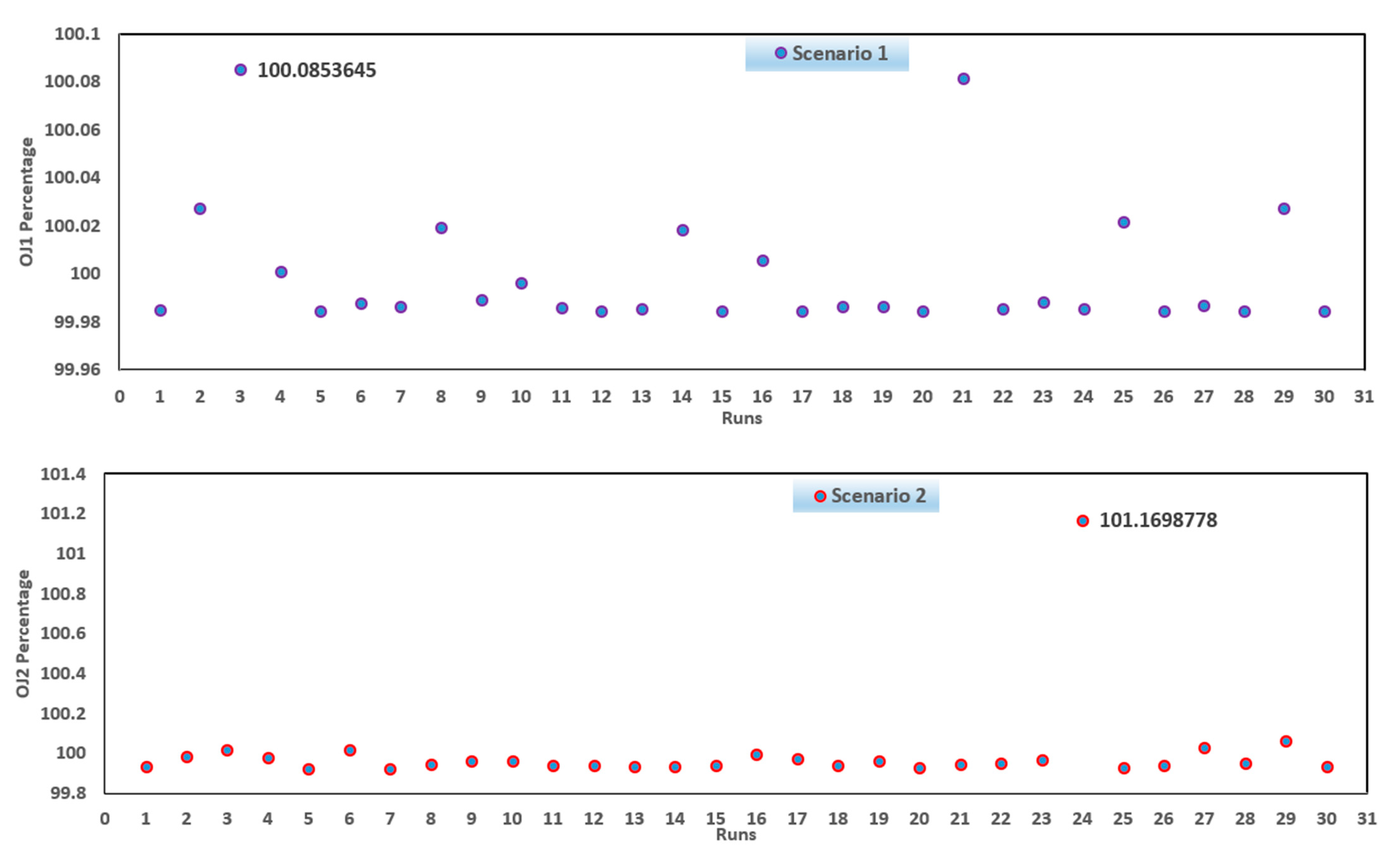
| |Mean-Worst| | 0.0853% | 1.1698% | 1.0667% | 8.6738% |
| |Best-Mean| | 0.0156% | 0.0750% | 0.1665% | 2.1139% |
| Variables | Initial | Fifth Scenario | Sixth Scenario | |
|---|---|---|---|---|
| Voltage setting of the generators (p.u) | Gen 1 | 1.0500 | 1.1000 | 1.0057 |
| Gen 2 | 1.0400 | 1.0960 | 1.0045 | |
| Gen 5 | 1.0100 | 1.0771 | 1.0003 | |
| Gen 8 | 1.0100 | 1.0881 | 1.0111 | |
| Gen 11 | 1.0500 | 1.1000 | 1.0007 | |
| Gen 13 | 1.0500 | 1.0546 | 1.0018 | |
| Output powers of the generators (MW) | Gen 1 | 99.2400 | 1.0553 | 1.0137 |
| Gen 2 | 80.0000 | 1.1000 | 0.9097 | |
| Gen 5 | 50.0000 | 1.1000 | 0.9814 | |
| Gen 8 | 20.0000 | 1.1000 | 0.9741 | |
| Gen 11 | 20.0000 | 6.243 × 10⁻⁹ | 5.0000 | |
| Gen 13 | 20.0000 | 0.0000 | 5.0000 | |
| Tap setting of the transformers (p.u) | Tr 6–9 | 1.0780 | 5.0000 | 5.0000 |
| Tr 6–10 | 1.0690 | 4.6221 | 5.0000 | |
| Tr 4–12 | 1.0320 | 0.0000 | 5.0000 | |
| Tr 28–27 | 1.0680 | 5.0000 | 5.0000 | |
| Output reactive powers of the VAR sources ar buses (MVAr) | Bus 10 | 0.0000 | 5.0000 | 5.0000 |
| Bus 12 | 0.0000 | 5.0000 | 5.0000 | |
| Bus 15 | 0.0000 | 5.0000 | 4.9517 | |
| Bus 17 | 0.0000 | 82.1327 | 81.8371 | |
| Bus 20 | 0.0000 | 62.7968 | 62.4782 | |
| Bus 21 | 0.0000 | 37.4611 | 38.7375 | |
| Bus 23 | 0.0000 | 35.0000 | 35.0000 | |
| Bus 24 | 0.0000 | 30.0000 | 30.0000 | |
| Bus 29 | 0.0000 | 40.0000 | 40.0000 | |
| Cost_Pg | 901.9600 | 890.1029 | 895.4292 | |
| Losses | 5.8324 | 3.9906 | 4.6529 | |
| Emissions | 0.2390 | 0.2127 | 0.2123 | |
| Fitness | 1.0000 | 0.7705 | 0.6691 | |
| Statistical Indices | Scenario 5 | Scenario 6 |
|---|---|---|
| Best | 0.7705 | 0.6691 |
| Mean | 0.7819 | 0.6896 |
| Worst | 0.7914 | 0.7473 |
| Standard deviation | 0.0909 | 0.0043 |
| Standard error | 0.0166 | 0.0008 |
| |Best-Worst| | 2.7057% | 11.6914% |
| |Mean-Worst| | 1.2176% | 8.3600% |
| |Best-Mean| | 1.4701% | 3.0743% |
| Variables | Initial | Fifth Scenario | |
|---|---|---|---|
| Voltage setting of the generators (p.u) | Gen 1 | 1.0000 | 1.0600 |
| Gen 2 | 1.0000 | 1.0599 | |
| Gen 3 | 1.0000 | 1.0599 | |
| Gen 4 | 1.0000 | 1.0599 | |
| Gen 5 | 1.0000 | 1.0599 | |
| Gen 6 | 1.0000 | 1.0599 | |
| Gen 7 | 1.0000 | 1.0455 | |
| Gen 8 | 1.0000 | 1.05173 | |
| Output powers of the generators (MW) | Gen 1 | 85.6900 | 189.5676 |
| Gen 2 | 157.400 | 10.0000 | |
| Gen 3 | 139.3100 | 214.6980 | |
| Gen 4 | 113.6900 | 180.4253 | |
| Gen 5 | 166.4800 | 10.0000 | |
| Gen 6 | 31.7100 | 234.0139 | |
| Gen 7 | 92.0000 | 56.3042 | |
| Gen 8 | 122.4900 | 32.1957 | |
| FGCs (USD/h) | 25,098.7000 | 22,953.4247 | |
| OPLs (MW) | 19.0150 | 37.4550 | |
| Technique | FGCs (USD/h) | Technique | FGCs (USD/h) |
|---|---|---|---|
| Developed GTOT | 22,953.4247 | ISHT [65] | 22,958.7800 |
| NBT [48] | 22,960.8100 | CST [47] | 22,959.3600 |
| SST [65] | 22,965.5900 | MCST [47] | 22,955.5500 |
| GWT [65] | 22,957.7200 |
| Variables | Initial | Sixth Scenario | |
|---|---|---|---|
| Voltage setting of the generators (p.u) | Gen 1 | 1.0000 | 1.0595 |
| Gen 2 | 1.0000 | 1.0600 | |
| Gen 3 | 1.0000 | 1.0600 | |
| Gen 4 | 1.0000 | 1.0600 | |
| Gen 5 | 1.0000 | 1.0600 | |
| Gen 6 | 1.0000 | 1.0600 | |
| Gen 7 | 1.0000 | 1.0600 | |
| Gen 8 | 1.0000 | 1.0600 | |
| Output powers of the generators (MW) | Gen 1 | 85.6900 | 60.4617 |
| Gen 2 | 157.4000 | 58.8194 | |
| Gen 3 | 139.3100 | 180.6455 | |
| Gen 4 | 113.6900 | 130.7554 | |
| Gen 5 | 166.4800 | 117.9838 | |
| Gen 6 | 31.7100 | 105.4722 | |
| Gen 7 | 92.0000 | 156.5709 | |
| Gen 8 | 122.4900 | 86.2761 | |
| FGCs (USD/h) | 25,098.7000 | 24,773.0865 | |
| OPLs (MW) | 19.0150 | 7.2353 | |
| Statistical Indices | Scenario 7 | Scenario 8 |
|---|---|---|
| Best | 22,953.4200 | 7.2353 |
| Mean | 22,956.5800 | 7.2353 |
| Worst | 22,984.9400 | 7.2353 |
| Standard deviation | 7.3505 | 1.28 × 10⁻⁵ |
| Standard error | 1.3420 | 2.33 × 10⁻⁶ |
| |Best-Worst| | 0.1373% | 0.0003% |
| |Mean-Worst| | 0.1235% | 0.0001% |
| |Best-Mean| | 0.0137% | 0.0002% |
| Variables | Initial | Ninth Scenario | |
|---|---|---|---|
| Voltage setting of the generators (p.u) | Gen 1 | 1.0000 | 1.0600 |
| Gen 2 | 1.0000 | 1.0600 | |
| Gen 3 | 1.0000 | 1.0600 | |
| Gen 4 | 1.0000 | 1.0600 | |
| Gen 5 | 1.0000 | 1.0599 | |
| Gen 6 | 1.0000 | 1.0600 | |
| Gen 7 | 1.0000 | 1.0599 | |
| Gen 8 | 1.0000 | 1.0600 | |
| Output powers of the generators (MW) | Gen 1 | 85.6900 | 67.2453 |
| Gen 2 | 157.4000 | 51.3626 | |
| Gen 3 | 139.3100 | 183.2907 | |
| Gen 4 | 113.6900 | 133.4820 | |
| Gen 5 | 166.4800 | 108.3223 | |
| Gen 6 | 31.7100 | 123.8325 | |
| Gen 7 | 92.0000 | 148.2581 | |
| Gen 8 | 122.4900 | 81.2601 | |
| FGCs (USD/h) | 25,098.7000 | 24,586.3700 | |
| OPLs (MW) | 19.0150 | 7.3036 | |
| Fitness | 1.0000 | 0.6818 | |
| Statistical Indices | Scenario 9 |
|---|---|
| Best | 0.6818 |
| Mean | 0.6818 |
| Worst | 0.6818 |
| Standard deviation | 1.9551 × 10⁻⁸ |
| Standard error | 3.5696 × 10⁻⁹ |
| |Best-Worst| | 6.1814 × 10⁻⁶% |
| |Mean-Worst| | 2.7401 × 10⁻⁶% |
| |Best-Mean| | 3.4413 × 10⁻⁶% |
Publisher’s Note: MDPI stays neutral with regard to jurisdictional claims in published maps and institutional affiliations. |
© 2022 by the authors. Licensee MDPI, Basel, Switzerland. This article is an open access article distributed under the terms and conditions of the Creative Commons Attribution (CC BY) license (https://creativecommons.org/licenses/by/4.0/).
Share and Cite
Shaheen, A.; Ginidi, A.; El-Sehiemy, R.; Elsayed, A.; Elattar, E.; Dorrah, H.T. Developed Gorilla Troops Technique for Optimal Power Flow Problem in Electrical Power Systems. Mathematics 2022, 10, 1636. https://doi.org/10.3390/math10101636
Shaheen A, Ginidi A, El-Sehiemy R, Elsayed A, Elattar E, Dorrah HT. Developed Gorilla Troops Technique for Optimal Power Flow Problem in Electrical Power Systems. Mathematics. 2022; 10(10):1636. https://doi.org/10.3390/math10101636
Chicago/Turabian StyleShaheen, Abdullah, Ahmed Ginidi, Ragab El-Sehiemy, Abdallah Elsayed, Ehab Elattar, and Hassen T. Dorrah. 2022. "Developed Gorilla Troops Technique for Optimal Power Flow Problem in Electrical Power Systems" Mathematics 10, no. 10: 1636. https://doi.org/10.3390/math10101636
APA StyleShaheen, A., Ginidi, A., El-Sehiemy, R., Elsayed, A., Elattar, E., & Dorrah, H. T. (2022). Developed Gorilla Troops Technique for Optimal Power Flow Problem in Electrical Power Systems. Mathematics, 10(10), 1636. https://doi.org/10.3390/math10101636