Modelling the Dynamic Interaction between Economic Policy Uncertainty and Commodity Prices in India: The Dynamic Autoregressive Distributed Lag Approach

Abstract

This study examines the dynamic interaction between oil, natural gas, and prices with Indian economic policy uncertainty (EPU). The study finds that gold prices and industrial production are fundamental drivers of Indian economic policy uncertainty in both the short and long runs, using a dynamic autoregressive distributed lag (ARDL) model with monthly data ranging from January 2003 to July 2020. Gold prices are positively related to the Indian EPU, while industrial production is negatively related to it. Thus, investors in the Indian economy should use gold as a hedge for portfolio diversification and as a safe haven during an economic crisis. We also find a significant positive interconnection between gold prices and crude oil prices in both the short run and the long run, while the significant positive impact of natural gas prices on crude oil prices manifests only in the long run. The evidence also indicates that the EPUs of the US and Europe positively affect the Indian EPU, while the EPU of China does not have a significant effect. Higher crude oil prices are associated with higher gas prices, whereas higher gold prices are negatively associated with the natural gas price and vice versa. Furthermore, the evidence shows that the Indian EPU does not have a significant effect on the changes in the prices of goods.

1. Introduction

Recently, the interconnections between economic policy uncertainty and commodity prices such as crude oil, gold, and natural gas prices have attracted the attention of researchers, policymakers, and investors. However, there is no consensus in the literature concerning the nexus between these variables. Most importantly, little or no attention is paid to the case of India, which is among the world’s largest consumers of these commodities. The stabilization and development of economies largely depends on economic policies, and economic policy uncertainty deters economic progress [1]. Hence, since the 2008 global financial crisis, researchers and policymakers across the world have become increasingly interested in understanding the relationship between economic policy uncertainty and macroeconomic fundamentals. The construction of the news-based EPU indexes by Baker et al. [2] facilitated the assessment of the relationship between EPU and macroeconomic factors. The EPU indexes have been widely used to examine the interconnection between macroeconomic variables and the EPU [3,4,5]. For instance, the EPU is associated with industrial production and employment [2], unemployment [6], stock market returns and volatility [7], assets [8], and bank loans [9], among other variables. Given the importance of crude oil in the global economy, fluctuations in crude oil prices have huge economic and financial implications. Thus, following the seminal work of Hamilton [10], which attributed the US recession to oil price shocks, numerous studies have established that oil price shocks affect many macroeconomic variables [11,12,13,14,15,16]. Recently, several studies focused on the interconnectedness between crude oil prices and the EPU, primarily on how oil price shocks affect an economy through the EPU [7,14,17,18,19,20]. Other studies [2,21,22,23] report that economic policy uncertainty has significant effects on the major macroeconomic variables. The EPU may have an immediate impact on economic activity and, thereby, affect the fluctuation of crude oil prices through demand conditions. At high EPU, investors face a high level of uncertainty, risk, and cost of investment and are likely to withdraw their investments. This slows down economic activity and affects crude oil prices accordingly [8].

Equally, the relationship between the gold price and EPU received research attention in the literature [24,25,26,27,28,29,30]. These studies on the relationship between the gold price and EPU, confirm that gold is a viable instrument for diversifying an investment portfolio and hedging against fluctuations in bond prices, exchange rates, stock prices, inflation, and oil prices during economic and political uncertainty.

However, there is no consensus in the literature concerning the interdependence of oil prices and EPU, as well as gold prices and EPU. The conclusions of the studies vary by the methodology applied and the views differ as to whether oil and gold prices have a positive or negative association or effect on the EPU or, conversely, whether the EPU has a significant negative or positive influence on oil and gold prices [31].

Most importantly, little or no attention is paid to the case of India concerning the nexus between oil prices, gold prices, and EPU. This constitutes a fundamental lacuna in the literature because India is currently the third-largest consumer of crude oil and the fourth-largest importer of gold. Therefore, the changes in the prices of oil and gold could have significant effects on the Indian economy and could drive the EPU in the country. Moreover, India is growing rapidly and is increasingly integrating into the developed economies in terms of global trade and investment. This, attracts the attention of international investors to the country [32]. The returns on investment hugely depend on the level of uncertainty, and gold is considered to be a safe haven tool for hedging against uncertainty in the global financial system and inflation risk, as it protects investors against financial losses [26,33]. It is, therefore, imperative to study the relationship between oil and gold prices and the EPU in India.

Natural gas prices, which are one of the most volatile of all the energy prices, are not extensively studied in the literature despite their importance. Natural gas is one of the crucial commodities, whose price has a tremendous effect on the macroeconomic activity of countries, and India is one of the major importers (14th top importer) of natural gas. Therefore, the study of the interconnection between natural gas prices will be of significant benefit to researchers and policymakers in India.

Additionally, separating the long-run and short-run effects of oil and gold prices on EPU and the effect of the EPU on crude oil and gold is important for understanding the dynamic interactions of these variables. Meanwhile, some studies (e.g., [34]) reveal that the interdependence of the EPU and various macroeconomic variables is time-varying and the spillover effect in the short-run is different from the long-run effect [34]. Finally, none of the studies use the dynamic autoregressive distributed lag (ARDL) model in examining the dynamic relationship between oil prices, gold prices, natural gas prices, and EPU. The dynamic ARDL offers advantages in modelling dynamic links, particularly when the orders of integration of variables differ.

Economic conditions in large economies have been shown to have global effects [14]. In particular, the EPU of the US, the largest economy of the world, has effects on almost all economies in the world. The Indian economy is highly integrated into the world economy. Thus, one should consider major world economic uncertainty conditions when examining the interaction of the EPU of India with its domestic macroeconomic variables and also with commodity prices. Moreover, how the Indian EPU responds to the EPU of the major economies is also of interest to policymakers and researchers. Therefore, we include the EPUs of the US, Europe, and China in our analysis in order to avoid model misspecification and examine how the Indian EPU is affected by the EPUs of the top three largest economies in the world.

As the large literature on energy [10,11,12] and gold as the most important portfolio asset [33,34] shows, these commodity classes are the ones most connected to the macroeconomic activity of a country. Energy has the most significant role as an input to almost any economic activity. On the other hand, gold is the undisputed investment asset of the last two centuries because of its safe haven role during financial crises. Growing affluence is driving growth in demand for gold in India, one of the largest markets for the metal.

In Indian culture, gold is seen as a store of value, a sign of wealth and prestige, and a necessary component of many rites. According to the World Gold Council, which has been tracking the gold consumption since 2005, the COVID-19 pandemic has revealed that pent-up demand for pendants and parties in India pushed bullion sales to their highest level on record in the fourth quarter of 2021. Over the course of the era, Indians acquired around 340 tons of gold, demonstrating the importance of gold to the Indian economy. India imported more than 70% of its oil usage in 2015, accounting for 5.5 percent of its gross domestic product (GDP). As a result, decreased crude oil prices should help the current account. According to the Petroleum Planning and Analysis Cell of the energy ministry, India’s oil import dependence has increased from 70% in 2015 to 83.7% in 2019. For every 1 US dollar drop in the price of a barrel of oil, India’s current account balance improves by 1 billion US dollars. India has experienced rapid economic growth since implementing pro-market policy reforms in the 1990s. In recent years, growth rates have generally been in the 6–8% range, greatly above those of many rich countries and the majority of developing countries. Given the country’s size, India’s rapid growth has had a significant impact on the global economy, causing a boom in commodity markets over the last decade. Higher commodity prices may stifle India’s burgeoning private consumption patterns, as households spend more on these things. This could cause the Indian economy’s good recovery to slow down. Commodity price declines could benefit India, a net commodity importer, by reducing inflationary pressures and reducing current account and fiscal deficits.

Against this backdrop, our study contributes to the literature by investigating the dynamic interaction of the Indian economic policy uncertainty with the major commodities. The study also contributes to the literature by filling the aforementioned research gaps by examining the dynamic interaction between oil prices, natural gas prices, gold prices, and Indian economic policy uncertainty using dynamic ARDL techniques. Another contribution of our study is the examination of the response of the Indian EPU to the EPUs of the US, Europe, and China.

The remaining part of the study is organized as follows: Section 2 presents a review of related literature. We discuss the data and methods in Section 3 and present and discuss the empirical results in Section 4, while Section 5 contains the conclusion and policy implications.

2. Brief Review of the Previous Literature

The interconnection among oil prices, gold prices, and EPU has been extensively studied. Therefore, we review the relevant literature to establish the current trend of research in the area and identify the research gap intended to be filled in this study. We start with the oil price–EPU nexus. Studies regarding the relationship between oil prices and economic policy uncertainty abound, and are divided into two strands. The first strand considers EPU as the determinant of oil prices, its returns, and volatility, while the second strand sees oil prices as the determinant of EPU. Concerning the first strand, Wei et al. [22] reported that, besides the demand and supply of oil and speculation as to the traditional determinants of oil prices, EPU plays a vital role in driving the volatility of the crude oil market. Similarly, Qadan and Nama [23] emphasized the relevance of EPU as a fundamental predictor of crude oil prices and returns. The second strand of literature focuses on the effect of crude oil, production, prices, and returns on the EPU using several econometric methods. For instance, Kang et al. [7] found that demand-side (oil-market specific and real aggregate) shocks significantly affect EPU, but supply-side shocks do not have a significant impact on the EPU. Similarly, Antonakakis et al. [14] used data from January 1997 to June 2013 to examine the dynamic relationship between oil prices and EPU in selected oil-importing and oil-exporting countries. Using the Diebold–Yilmaz spillover index, the study found that EPU responds negatively to aggregate demand price shocks and that the oil price responds similarly to EPU shocks. Moreover, the spillover effect was unprecedented during the 2007–2009 global economic meltdown. However, the findings show that EPU was the dominant transmitter of shocks in the pre-2009 recession, while demand and supply shocks play a significant role in the transmission of the spillover effect in the post-2009 era. Aloui et al. [17] also used the copula approach to determine the relationship between oil price and EPU. They reported that the interdependence between crude oil returns and EPU is negative over the entire period of their study, but that the relationship is positive for the period before the 2007 global financial crisis. That is(means), higher EPU significantly decreases the crude oil returns over the entire study period, but higher EPU prior to the global recession results in an increase in the crude oil returns. In addition, Kang et al. [18] used a structural vector autoregressive (SVAR) model to examine the impact of crude oil production shocks on EPU. They examined the cases of US and non-US oil production shocks and found a negative association between the US oil production shocks and the EPU of the US. Further, the study reveals that oil supply shocks (US and non-US) explain the variation in the EPU as much as the structural demand shocks in the oil market. Recently, Hailemariam et al. [19] considered the relationship between oil prices and the EPU of G7 countries for the period between January, 1997 and June, 2018 using nonparametric panel data techniques. The study, found that oil prices have a different effect on EPU at different times. This is especially true when oil prices are driven by a rise in global aggregate demand.

Over the years, the relationship between the gold price and the EPU has also piqued the interest of academics and policymakers. Many studies document the link between gold prices and economic policy uncertainty for several countries across the globe, with mixed findings. For instance, Balcilar et al. [24] used a novel nonparametric quantiles-based causality test to examine the effects of policy and equity-market uncertainty on the returns and volatility of gold prices for different frequencies of data (daily and monthly). They discovered strong empirical evidence, which demonstrates that causality runs from uncertainty to gold price returns and volatility. However, they found that the causality weakens when quarterly data is used. Furthermore, Raza et al. [1] examined the causal relationship between EPU and gold prices using both Granger causality and the causality-in-quantiles techniques. They documented that Granger causality indicates the absence of causality between gold prices and EPU. Conversely, the causality-in-quantiles technique indicates that causality runs from the EPU to the gold price, especially at the low-tails. Moreover, Fang et al. [35] also reported that global EPU positively affects the forecast of the volatility of the gold futures market. Similarly, Jones and Sackley [36] found a positive association between EPU and the gold price. Higher uncertainty leads to an increase in the gold price. However, Wu et al. [37] used GARCH and quantile regression models to evaluate the hedge and safe haven characteristics of gold prices and bitcoin in the face of EPU. The study reveals that the gold price does not serve as a strong hedge or safe haven for the EPU. The gold price can only serve as a weak hedge and a weak safe haven against EPU during the extreme bullish and bearish markets. Other studies [29], found that the role of the gold price in the fluctuation of the EPU varies over time. They show that the role of gold prices changed significantly after the 2007–2009 global recession. The study indicates that gold prices have a positive relationship with overall EPU, but a negative association with macroeconomic and inflation uncertainties. The interaction between oil prices and gold prices is also established in the literature [30].

The nexus between natural gas prices and EPU has not been extensively examined in the literature. Reboredo and Uddin [38] is one of the few studies that incorporated natural gas prices into their analysis of the impact of EPU and financial stress on energy and precious metal prices in the US. They used the quantile regression approach and found that there is no co-movement between the policy uncertainty and the commodity prices.

From the above literature review, it is revealed that none of the existing studies considers the case of India with regard to the dynamic relationship among the Indian EPU, commodity prices, and EPUs of major economies. The results of the extant studies vary according to the methods and period of the study. More importantly, the literature almost entirely ignores the relationship between natural gas prices and EPU. As a result, this study investigates the dynamics of the relationship between Indian EPU, gold prices, oil prices, and natural gas prices after controlling for the effects of other domestic macroeconomic factors and the EPUs of the world’s major economies, namely the US, Europe, and China. This is imperative given the critical position of the Indian economy in the world market for oil, gold, and natural gas. The study provides policymakers and investors an in-depth look at the variables so that they can make better decisions.

3. Materials and Methods

To examine the dynamic relationship between economic policy uncertainty and commodity and energy prices, we estimated the models using monthly data on Indian EPU, US EPU, European EPU, Chinese EPU, oil prices, natural gas prices, and gold prices for the period from January 2003 to July 2020. The choice of the variables was guided by previous studies, while the period (2003–2020) was used based on the availability of EPU data for India. We used the news-based measure of EPUs for India, the US, Europe, and China [2]. The West Texas Intermediate (WTI) spot price of crude oil in US dollars per barrel and the Henry-Hub natural gas spot price per million metric British thermal units (Btu) were sourced from the United States Energy Information Administration (EIA). The monthly gold price in US dollars per troy ounce was obtained from the Chicago Mercantile Exchange (CME) group commodity database. Furthermore, in the model with Indian EPU as the dependent variable, we used the industrial production index and the real interest rate as control variables. Both variables were obtained from the Organization for Economic Co-operation and Development (OECD) database. Meanwhile, all the variables except interest rate, were log transformed to linearize the possible nonlinear relationships, stabilize the variance, and ensure easy interpretation of the empirical results in elasticities.

3.1. Unit Root Tests

Time series literature stresses the importance of testing for non-stationarity of the series and the existence of cointegration, to ensure the ultimate choice of appropriate models for estimations. Failure to perform the pretesting, increases the likelihood of the choice of the wrong methods and spurious inference [39]. Thus, we started the analysis in this study with non-stationarity tests. This was necessary for the examination of the attributes of the series, to avoid spurious regression results. The regression of a nonstationary variable on another nonstationary variable or variables may produce spurious estimates, which lead to misleading inferences. To avoid this, we used the augmented Dickey–Fuller (ADF) test [40], the Phillips–Perron (PP) test [41], and the Kwiatkowski–Phillips–Schmidt–Shin (KPSS) test [42], in order to examine the stationarity properties of all the variables.

3.2. Cointegration Tests

After ascertaining the stationarity characteristics of the variables, we conducted cointegration tests to examine the existence or otherwise(inexistence) of a long-run equilibrium relationship among the variables in each model. The short-run fluctuations may create disequilibrium, which may be corrected as the series moves backward to a stable equilibrium. The existence of a stable long-run equilibrium signifies cointegration among the series in the model [39,43]. However, not all nonstationary data series validate the existence of cointegration. Thus, it becomes imperative to test for the cointegrating relationship among the series. Therefore, we use the ARDL bounds test approach [44] and the Bayer–Hanck [45] combined cointegration test. Unlike the conventional Engle–Granger [46] and Johansen [47] cointegration tests, which require that the variables be integrated of the same order, the ARDL bounds test is flexible to the stationarity properties of the series because it can be applied for variables with a different order of integration (I (0) and I (1)) or the same order of integration (I (0) and I (0), or I (1) and I (1)). It also has desirable small sample and asymptotic properties with consistent long-run estimates [39,44]. Meanwhile, we applied the dynamic ARDL specification to conduct the bounds test for cointegration using the critical values and the approximate p-values suggested by [48]. To reject the null hypothesis of no cointegration, the F-statistic must be greater than the critical value of the upper bound, and the approximate p-value must be statistically significant [48].

We also applied the Bayer–Hanck [45] combined test for cointegration, to ensure robustness of the cointegration test results and avoid the tendency of the ARDL bounds test to produce inconclusive results [45]. The test is a combination of the Engle–Granger [46], Johansen [47], Boswijk [49], and Banerjee–Dolado–Mestre [50] cointegration tests. The Bayer–Hank Fisher’s statistic is computed by combining the probability values (p-values) of the individual tests using the following formulas:

$$F_{EG-J}=-2\left[\ln \left(P_{EG}\right)+\ln \left(P_J\right)\right]$$

(1)

$$F_{EG-J-B-BDM}=-2\left[\ln \left(P_{EG}\right)+\ln \left(P_J\right)+\ln \left(P_B\right)+\ln \left(P_{BDM}\right)\right]$$

(2)

In Equations (1) and (2), we indicate the p-values of the Engle–Granger, Johansen, Boswijk, and Benerjee cointegration tests by $P_{EG}$, $P_J$, $P_B$ and $P_{BDM}$, respectively. The null hypothesis of no cointegration is rejected when the computed F-statistic is greater than the critical value of the statistic provided by [45] for the conventional levels of significance (1%, 5%, and 10%). The rejection of the null hypothesis, indicates the existence of a long-run equilibrium relationship among the series in the model.

3.3. The Empirical Dynamic ARDL Model Specification

The ARDL models, in general, contain complicated specifications that incorporate numerous delays, initial differences, and lagged differences. As a result, interpreting the short- and long-run implications of changes in the independent variables becomes increasingly complex. Jordan and Philips [43] developed the dynamic simulated ARDL model, which simulates a number of ARDL models, including an error-correction model, to alleviate the challenges associated with the complexity of the traditional ARDL model. The dynamic simulation provides an alternative hypothesis test of model coefficients by conveying the statistical importance of the estimates through realistic counterfactual situations. While holding other independent variables constant, it estimates, simulates, and graphs the prediction of counterfactual changes in one independent variable on the dependent variables. The ARDL model with dynamic simulations is used in this study’s econometric analysis due to its various advantages. The ARDL model in general is as follows:

$$\Delta y_t={\alpha }_0+{\theta }_0{y}_{t-1}+{\theta }_1{x}_{1t-1}+\cdots +{\theta }_k{x}_{kt-1}+{{\displaystyle \sum }}_{i=1}^p{\alpha }_i\Delta y_{t-1}+{{\displaystyle \sum }}_{j=0}^{q_1}{\beta }_{1j}\Delta x_{1t-j}+\cdots +{{\displaystyle \sum }}_{j=0}^{q_{\mathrm{k}}}{\beta }_{kj}\Delta x_{kt-j}+{\epsilon }_t$$

(3)

Equation (3) expresses the first difference ($\Delta$) of the dependent variable $y_t$ at time $t=1, 2,\dots ,T$ as a function of an intercept $\left({\alpha }_0\right)$, the first lag of the dependent variable in levels ($y_{t-1}$), the first lag of independent variables in levels, $x_{1t-1},x_{2t-1},\dots ,x_{kt-1}$, and up to maximum lags $p$ and $q_i$, $i=1, 2,\dots ,k$, of the first differences of dependent and independent variables, respectively, with an error term ${\epsilon }_t$. The first differences are included to account for autocorrelation and delayed effects [39].

We estimate the dynamic relationship between each of the prices (oil, gold, and natural gas), the US EPU (usepu), European EPU (euepu), Chinese EPU (cepu), and the India EPU (iepu) using the dynamic ARDL specified in Equation (3). The dependent variables are IEPU, crude oil price (cop), gold price (gp), and natural gas price (ngp) all in their log forms. Meanwhile, we choose a maximum of one lag for all the models based on the Schwarz’s Bayesian information criterion (SBC). We specified each empirical model based on previous empirical studies. Thus, following [19,51,52] the econometric model for the evaluation of the effect of the prices of oil, gold, and natural gas on the Indian EPU is specified as follows:

$$\begin{array}{cc}\hfill \Delta lniep{u}_t={\alpha }_0+& {\theta }_{0}lniep{u}_{t-1}+{\theta }_{1}lnco{p}_{t-1}+{\theta }_{2}lng{p}_{t-1}+{\theta }_{3}lnng{p}_{t-1}+{\theta }_{4}lnip{i}_{t-1}+{\theta }_{5}int{r}_{t-1}\hfill \\ & +{\theta }_{6}lnusep{u}_{t-1}+{\theta }_{7}lneuep{u}_{t-1}+{\theta }_{8}lncep{u}_{t-1}+{\beta }_1\Delta lnco{p}_{t-1}+{\beta }_2\Delta lng{p}_{t-1}+{\beta }_3\Delta lnng{p}_{t-1}\hfill \\ & +{\beta }_4\Delta lnip{i}_{t-1}+{\beta }_5\Delta int{r}_{t-1}+{\beta }_6\Delta lnusep{u}_{t-1}+{\beta }_7\Delta lneuep{u}_{t-1}+{\beta }_8\Delta lncep{u}_{t-1}+{\epsilon }_t\hfill \end{array}$$

(4)

where $lniepu$, $lncop$, $lngp,$ $lnngp$, $lnusepu$, $lneuepu$, and $lncepu$n symbolize the Indian EPU, crude oil price, gold price, natural gas price, US EPU, European EPU, and Chinese EPU in natural logarithms. The Indian industrial production index in log and the real interest rate are denoted by $lnipi$ and $intr$, respectively.

For the model linking the oil price to the EPU, we follow [22,23,53,54,55] to specify the empirical econometric model as follows:

$$\begin{array}{cc}\hfill \Delta lnco{p}_t={\alpha }_0+& {\theta }_{0}lnco{p}_{t-1}+{\theta }_{1}lniep{u}_{t-1}+{\theta }_{2}lng{p}_{t-1}+{\theta }_{3}lnng{p}_{t-1}+{\theta }_{4}lnusep{u}_{t-1}+{\theta }_{5}lneuep{u}_{t-1}\hfill \\ & +{\theta }_{6}lncep{u}_{t-1}+{\beta }_1\Delta lniep{u}_{t-1}+{\beta }_2\Delta lng{p}_{t-1}+{\beta }_3\Delta lnng{p}_{t-1}+{\beta }_4\Delta lnusep{u}_{t-1}\hfill \\ & +{\beta }_5\Delta lneuep{u}_{t-1}+{\beta }_6\Delta lncep{u}_{t-1}+{\epsilon }_t\hfill \end{array}$$

(5)

Similarly, based on the empirical model of [1,24,36,37,56,57,58,59] the following model is specified to examine the impact of EPU on gold price:

$$\begin{array}{cc}\hfill \Delta lng{p}_t={\alpha }_0+& {\theta }_{0}lng{p}_{t-1}+{\theta }_{1}lniep{u}_{t-1}+{\theta }_{2}lnco{p}_{t-1}+{\theta }_{3}lnn{p}_{t-1}+{\theta }_{4}lnusep{u}_{t-1}+{\theta }_{5}lneuep{u}_{t-1}\hfill \\ & +{\theta }_{6}lncep{u}_{t-1}+{\beta }_1\Delta lniep{u}_{t-1}+{\beta }_2\Delta lnco{p}_{t-1}+{\beta }_3\Delta lnng{p}_{t-1}+{\beta }_4\Delta lnusep{u}_{t-1}\hfill \\ & +{\beta }_5\Delta lneuep{u}_{t-1}+{\beta }_6\Delta lncep{u}_{t-1}+{\epsilon }_t\hfill \end{array}$$

(6)

Likewise, the model specification of [38] is adopted to model the impact of Indian EPU on natural gas price as indicated in Equation (7):

$$\begin{array}{cc}\hfill \Delta lnng{p}_t={\alpha }_0+& {\theta }_{0}lnng{p}_{t-1}+{\theta }_{1}lniep{u}_{t-1}+{\theta }_{2}lnco{p}_{t-1}+{\theta }_{3}lng{p}_{t-1}+{\theta }_{4}lnusep{u}_{t-1}+{\theta }_{5}lneuep{u}_{t-1}\hfill \\ & +{\theta }_{6}lncep{u}_{t-1}+{\beta }_1\Delta lniep{u}_{t-1}+{\beta }_2\Delta lnco{p}_{t-1}+{\beta }_3\Delta lng{p}_{t-1}+{\beta }_4\Delta lnusep{u}_{t-1}\hfill \\ & +{\beta }_5\Delta lneuep{u}_{t-1}+{\beta }_6\Delta lncep{u}_{t-1}+{\epsilon }_t\hfill \end{array}$$

(7)

The industrial production index and the interest rate are not included in Equations (5)–(7) because the dependent variables in these equations are global prices, on which the Indian macroeconomic variables alone can only have a negligible impact. Analogous to the previous studies, this study does not include the domestic macroeconomic variables of any country to determine the fluctuation of global commodity and energy prices.

4. Results

Table 1. Descriptive statistics.

Variables	Mean	Standard Deviation	Min	Max	p1	p99	Skewness	Kurtosis
iepu	93.353	50.793	24.940	283.690	30.690	249.340	1.289	4.662
cop	66.801	23.953	16.550	133.880	28.170	125.400	0.377	2.386
gp	1069.565	417.150	328.180	1843.310	351.020	1755.810	−0.312	1.979
ngp	4.601	2.277	1.630	13.420	1.740	12.690	1.363	5.107
ipi	86.343	20.606	46.300	127.360	47.370	121.440	−0.286	2.078
intr	6.758	1.163	5.400	10.250	5.400	9.500	1.240	3.010
usepu	133.110	66.178	44.783	503.963	49.599	425.779	2.242	10.836
euepu	164.263	70.451	47.692	433.277	58.518	392.831	0.758	4.016
cepu	233.176	227.922	26.144	970.830	32.729	935.310	1.751	5.184

Note: iepu denotes Indian economic policy uncertainty, cop denotes crude oil price, gp denotes gold price, ngp denotes natural gas price, ipi denotes industrial production index, and intr denotes interest rate. usepu denotes the economic policy uncertainty index of the US, euepu denotes the economic policy uncertainty index of Europe, and cepu denotes the economic policy uncertainty index of China. The p1 and p99 denote 1% and 99% percentiles, respectively.

contains the descriptive statistics of the variables used in the study. It indicates that the average Indian economic uncertainty index is 93.353 with a minimum of 24.94 and a maximum of 283.69. This implies that there has been a high level of economic policy fluctuations and uncertainty in India over the years considered. However, the Indian EPU is less volatile than the EPUs of the US, Europe, and China, which have standard deviations of 66.178, 70.451, and 227.922, respectively. On average, over the period, the crude oil price was 66.801 USD per barrel, with 16.55 and 133.88 USD per barrel as the minimum and maximum, respectively. Moreover, gold prices ranged from 328.18 to 1843.31 USD per troy ounce, with an average of 1069.565 USD per troy ounce during the period. The natural gas spot price fluctuated between 1.63 and 13.42, averaging 4.601 USD per million metric British thermal units (Btu). The average industrial production index (ipi) over the period was 86.343, while the minimum and maximum ipi were 46.3 and 127.36, respectively. Interest rates ranged from 5.4 to 10.2, with an average of 6.758 percent. In addition, the skewness and kurtosis show that all the series are not normally distributed. The gold price and industrial output are negatively skewed, whereas other variables are positively skewed. All economic policy uncertainty series and natural gas prices have fat-tailed distributions (leptokurtic with a kurtosis greater than three), while all other variables have thin-tailed distributions (platykurtic with a kurtosis less than three). Therefore, the descriptive statistics indicate that the period considered in this study covers a period during which there were significant fluctuations in both global commodities and Indian domestic variables such as the interest rate, industrial production index, and economic policy uncertainty. The oscillations in the series are further indicated by the large values of the standard deviations of all the variables.

Before proceeding to the main analysis, we conduct non-stationarity tests for all the variables using the three most commonly used unit root tests, namely, augmented Dickey–Fuller, Phillips–Perron, and the KPSS unit root tests. All the tests were conducted with three deterministic term specifications: constantly only (C), constant and trend (CT), and no deterministic term (no constant and trend). This was to ensure the robustness of the estimates. The results are reported in

Table 2. Unit root tests.

	Tests for the Levels of Series			Tests for the First Differences of Series
	Constant Deterministic Term	Constant and Trend Deterministic Term	No Deterministic Term	Constant Deterministic Term	Constant and Trend Deterministic Term	No Deterministic Term
Phillips Perron (PP)
lncop	−2.5791	−2.4422	−0.0910	−10.4433 ***	−10.526 ***	−10.4790 ***
lngp	−1.6396	−1.4268	2.5303	−12.4691 ***	−12.492 ***	−12.1850 ***
lniepu	−6.1959 ***	−6.2493 ***	0.0841	−35.647 ***	−35.484 ***	−35.6140 ***
intr	−1.5965	−1.4859	−0.2090	−10.4251 ***	−10.409 ***	−10.4560 ***
lnipi	−2.2994	−4.2045 ***	0.4281	−27.7764 ***	−30.357 ***	−27.3630 ***
lnngp	−1.5950	−3.6449 **	−1.0790	−15.6508 ***	−15.63 ***	−15.6380 ***
lnusepu	−4.3151 ***	−6.0298 ***	−0.0170	−19.4184 ***	−19.4535 ***	−19.4613 ***
lneuepu	−3.2363 ***	−5.9237 ***	0.0065	−20.9361 ***	−20.9703 ***	−20.9945 ***
lncepu	−3.1847 ***	−6.9353 ***	0.1285	−25.7671 ***	−25.7841 ***	−25.7688 ***
Augmented Dickey Fuller (ADF)
lncop	−2.9594 **	−2.9115	−0.2051	−10.8690 ***	−10.8837 ***	−10.8950 ***
lngp	−1.6819	−1.3518	2.8292	−12.4932 ***	−12.5264 ***	−12.0790 ***
lniepu	−3.0675 **	−3.1206 **	−0.2163	−17.2384 ***	−17.1980 ***	−17.2803 ***
intr	−1.9519	−1.8944	−0.2487	−10.8137 ***	−10.8054 ***	−10.8397 ***
lnipi	−1.9166	0.3259	−0.1935	−10.1879 ***	−12.0273 ***	−11.4883 ***
lnngp	−1.6514	−3.5186 **	−1.0786	−15.6688 ***	−15.6297 ***	−15.6564 ***
lnusepu	−2.9210 ***	−4.6483 ***	0.0392	−12.2622 ***	−12.3637 ***	−12.2824 ***
lneuepu	−1.7589 ***	−4.3515 ***	0.0993	−8.5441 ***	−8.5331 ***	−8.5542 ***
lncepu	−1.1029	−3.2834 *	0.5148	−9.7971 ***	−9.8425 ***	−9.7794 ***
Kwiatkowski, Phillips, Schmidt, Shin (KPSS)
lncop	0.3254	0.3260 ***		0.1546	0.0312
lngp	1.4045 ***	0.4101 ***		0.2888	0.1331
lniepu	0.3535	0.3117 ***		0.1296	0.1234
intr	0.5483	0.2397 ***		0.1334	0.0916
lnipi	1.6044 **	0.3773 ***		0.3840	0.1235
lnngp	1.4526 ***	0.0884		0.0470	0.0280
lnusepu	2.6113 ***	0.2374 ***		0.0856	0.0245
lneuepu	2.9304 ***	0.1782 **		0.0451	0.0320
lncepu	3.6073 ***	0.402 ***		0.0601	0.0171

Note: The prefix “LN” indicates natural log. ***, ** and * denote 1%, 5% and 10% level of significance, respectively. See Note to Table 1.

. The essence of the unit root tests is to examine the stationarity properties of the series for the purpose of choosing the appropriate models and techniques of analysis and avoiding spurious regression results often associated with nonstationary series. The results of the PP tests show that only all economic uncertainty series (lniepu, lnusepu, lneuepu, and lncepu), industrial production, and natural gas prices are stationary at their levels when the constant only and constant with trend specifications are used, but none of the variables are level stationary for the option of none (no constant and trend). Similarly, ADF and KPSS indicate that some variables are stationary in levels with constant only (lncop, liniepu, intr, lnusepu, and lncepu) and with constant and trend (lnngp, lniepu, lnusepu, and lncepu), while all the variables, except lnngp for KPSS, are not stationary in levels for the no deterministic term specification. However, all the variables are stationary in first difference for all the tests and all deterministic term specifications. This indicates that the series are at most integrated of order one (I (1)), while some of them are integrated of order zero (I (0)). In sum, the variables are robustly first-difference stationary and thus fulfill the requirements of the dynamic ARDL used in this study.

The results of the stationarity tests indicate that some of the variables are I (0) and others I (1), but none are of an order of integration greater than 1, indicating that all variables are robustly stationary in the first difference. In such a case, it is important to examine the existence of a long-run relationship among the variables in all the model specifications given in Equations (4)–(7). Thus, we conduct cointegration tests to ascertain the existence of a long-run equilibrium relationship among the variables in all four models.

Table 3. Cointegration tests.

Models	Statistics	5% Critical Value		p-Value
Bounds tests for levels relationship
Model 1		I (0)	I (1)	I (0)	I (1)
F-statistic	9.999	2.241	3.470	0.000	0.000
t-statistic	−9.379	−2.846	−4.720	0.000	0.000
Model 2
F-statistic	4.116	2.481	3.690	0.001	0.023
t-statistic	−4.640	−2.854	−4.396	0.000	0.029
Model 3
F-statistic	2.300	2.481	3.690	0.073	0.384
t-statistic	−0.128	−2.854	−4.396	0.937	0.995
Model 4
F-statistic	5.843	2.481	3.690	0.000	0.001
t-statistic	−5.179	−2.854	−4.396	0.000	0.007
Bayer–Hanck Test for Cointegration
	EG-J	5% Critical Value	EG-J-B-BDM	5% Critical Value	Remarks
Model 1	12.454	10.181	33.569	19.447	Cointegrated
Model 2	33.258	10.352	58.613	19.761	Cointegrated
Model 3	27.553	10.352	28.561	19.761	Cointegrated
Model 4	32.682	10.352	60.314	19.761	Cointegrated

Note: Model specifications; Model 1: lniepu = f (lncop, lngp, lnngp, lnipi, intr, lnusepu, lneuepu, lncepu), Model 2: lncop = f (lniepu, lngp, lnngp, lnusepu, lneuepu, lncepu), Model 3: lngp = f (lniepu, lncop, lnngp, lnusepu, lneuepu, lncepu), and Model 4: lnngp = f (lniepu, lncop, lngp, lnusepu, lneuepu, lncepu). EG-J denotes the Engle–Granger–Johansen test and EG-J-B-BDM denotes the Engle–Granger–Johansen–Boswijk–Benerjee–Dolado–Mestre test.

contains the results of the ARDL bounds test for cointegration with critical values and approximate p-values taken from Kripfganz and Schneider [48] and the Bayer–Hanck combined test for cointegration.

The results of the ARDL bounds test reveal that there is cointegration among the variables at the 5% level in all the models except Model 3, where the log of gold price is the dependent variable. However, the Bayer–Hanck test reveals that the F-statistics of both the EG-J and EG-J-B-BDM are greater than the 5% critical values for all the models. This shows the existence of cointegration among the variables in all the models. The results of the tests for cointegration imply that there is a long-run equilibrium relationship among all the variables in all the models. This necessitates the estimation of the short-run and long-run coefficients using the dynamic ARDL model used in the current study.

Table 4. Estimates of dynamic ARDL model.

	Model 1	Model 2	Model 3	Model 4
Dependent Variable:	$\mathbf{\Delta }\mathit{l}\mathit{n}\mathit{i}\mathit{e}\mathit{p}{\mathit{u}}_{\mathit{t}}$	$\mathbf{\Delta }\mathit{l}\mathit{n}\mathit{c}\mathit{o}{\mathit{p}}_{\mathit{t}}$	$\mathbf{\Delta }\mathit{l}\mathit{n}\mathit{g}{\mathit{p}}_{\mathit{t}}$	$\mathbf{\Delta }\mathit{l}\mathit{n}\mathit{n}\mathit{g}{\mathit{p}}_{\mathit{t}}$
Long-run estimates
$lnco{p}_{t-1}$	0.531 **	−0.194 ***	−1.635	1.016 ***
	(2.338)	(−4.640)	(−0.0844)	(6.204)
$lng{p}_{t-1}$	0.616 **	1.005 ***	−0.00217	−1.131 ***
	(2.028)	(7.485)	(−0.128)	(−6.713)
$lnng{p}_{t-1}$	0.0159	0.507 ***	0.305	−0.217 ***
	(0.074)	(3.493)	(0.036)	(−5.179)
$lnip{i}_{t-1}$	−1.532 ***
	(−3.806)
$int{r}_{t-1}$	0.0297
	(0.693)
$lnusep{u}_{t-1}$	0.366 *	−0.204	19.37	−0.0676
	(1.671)	(−1.077)	(0.128)	(−0.344)
$lneuep{u}_{t-1}$	0.379 *	−0.374 *	14.55	−0.428 *
	(1.707)	(−1.706)	(0.126)	(−1.786)
$lncep{u}_{t-1}$	−0.0445	−0.059	0.0333	−0.132
	(−0.477)	(−0.713)	(0.013)	(−1.524)
$lniep{u}_{t-1}$	−0.612 ***	−0.0796	−4.36	−0.184
	(−9.379)	(−0.738)	(−0.127)	(−1.593)
Short-run estimates
$\mathsf{\Delta }lnco{p}_{t-1}$	0.0788		0.0216	0.270 ***
	(0.309)		(0.844)	(3.454)
$\mathsf{\Delta }lng{p}_{t-1}$	−0.0904	0.167		0.192
	(−0.141)	(0.844)		(0.862)
$\mathsf{\Delta }lnng{p}_{t-1}$	−0.0305	0.213 ***	0.0196
	(−0.148)	(3.454)	(0.862)
$\mathsf{\Delta }lnip{i}_{t-1}$	−0.840 ***
	(−2.656)
$\mathsf{\Delta }int{r}_{t-1}$	0.177 *
	(1.758)
$\mathsf{\Delta }lnusep{u}_{t-1}$	0.384 ***	−0.0820 ***	0.0285 **	−0.0566
	(3.295)	(−2.304)	(2.222)	(−1.402)
$\mathsf{\Delta }lneuep{u}_{t-1}$	0.0543	−0.00793	0.000624	−0.0153
	(0.406)	(−0.192)	(0.0420)	(−0.329)
$\mathsf{\Delta }lncep{u}_{t-1}$	−0.029	−0.00338	−0.00427	−0.0286
	(−0.508)	(−0.195)	(−0.685)	(−1.472)
$\mathsf{\Delta }lniep{u}_{t-1}$		−0.00664	−0.00179	−0.00256
		(−0.307)	(−0.230)	(−0.106)
Constant	0.683	−0.134	0.0344	0.861 ***
	(0.826)	(−0.624)	(0.444)	(3.672)
Observations	210	210	210	210
R-squared	0.624	0.929	0.994	0.939
Ljung–Box test	18.405	26.162	19.884	22.020
Breusch–Pagan test	1.360	5.150	0.001	0.060
Replications	5000	5000	5000	5000

Note: The prefix ln indicates natural log while ∆ is the first difference operator. The variable names lniepu, lncop, lngp, lnngp, and lnipi symbolize the Indian EPU, crude oil price, gold price, natural gas price, and industrial production index in natural logarithms. t-statistics are in parenthesis. The Ljung–Box test is the test for autocorrelation in the regression residuals up to order 20, while the Breusch–Pagan test is the test for heteroskedasticity in the regression residuals. ***, ** and * denote 1%, 5% and 10% level of significance, respectively.

contains the estimates of the dynamic simulated ARDL for all the models. In Table 4, we report the Ljung–Box test for autocorrelation up to order 20, and the Breusch–Pagan test for heteroskedasticity in order to check whether the residuals are white noise. None of the Ljung–Box and Breusch–Pagan tests are rejected at the traditional significance levels, indicating that the residuals of all four models are white noise. The estimates for Model 1, where Indian economic policy uncertainty is used as a dependent variable, are contained in the first column. The coefficient of the lagged Indian EPU is negative (−0.612) and statistically significant at the 1% level. This indicates that about 61.2% of short-run disequilibrium is corrected every month as the variables move back to a stable long-run equilibrium relationship.

In the short run, the coefficients of gold prices, natural gas prices, and industrial production are negative, while the parameter estimates of crude oil prices and interest rates are positive. This implies that gold prices, natural gas prices, and industrial production are negatively associated with Indian economic policy uncertainty in the short run, while crude oil prices and interest rates are positively related to it. In other words, gold prices, natural gas prices, and industrial production reduce the economic policy uncertainty in India in the short run, while higher crude oil prices and interest rates increase the economic policy uncertainty in the country. The estimates indicate that the short-run effect of the US and European EPUs on the Indian EPU is positive, while that of the Chinese EPU is negative. However, only the coefficient of industrial production and the EPU of the US are statistically significant, indicating that only industrial production and the US economic policy uncertainty have a significant effect on the Indian EPU. Other variables are statistically insignificant and thus do not significantly affect the changes in the Indian EPU in the short run.

The long-run estimates of Model 1 show that the coefficients of crude oil prices, gold prices, natural gas prices, and interest rates are positive. This shows that an increase in all the commodity prices (crude oil, gold, and gas) leads to an increase in EPU in India and vice versa. On the other hand, a higher (lower) industrial production index causes a decline (increase) in the Indian EPU in the long run. The result shows that the coefficients of crude oil prices, gold prices, and industrial production are statistically significant at the 5% level of significance. This shows that, in the long run, crude oil prices, gold prices, and industrial production have a significant impact on the Indian EPU. Higher crude oil prices are well documented to lead to deteriorating economic activity, implying increased economic policy uncertainty. Results also suggest that with higher gold returns, economic policy uncertainty in India rises. There could be two reasons for this result. First, at high gold prices, investors are attracted to directing their investment to gold, which serves as a safe haven or hedge for the protection of their investment against uncertainties. This causes a drop in investments and escalates economic policy uncertainty. Second, high gold prices could signal a better performance of investment in gold-exporting countries. Thus, investors shift to such countries from the gold-importing economies such as India. This also increases the level of Indian economic policy uncertainty. This conforms to the findings of Demir et al. [58] and Wu et al. [37], which associate high gold prices with rising EPU and argue that gold can serve as a safe haven during severe economic crises and as a hedge for portfolio diversification during calm periods. Estimates also show that the EPU spillover from the US and Europe to India is positive and statistically significant at the 10% level, while a small but insignificant EPU spillover from China is indicated. The Chinese economy, with its tremendous trade surplus, might indicate increased trade potential and lower energy prices for India, implying a negative EPU spillover.

We report the estimates of Model 2 in the second column of Table 4, with crude oil prices as the dependent variable. The speed of adjustment (coefficient of the error-correction term) of the model is indicated by the coefficient of the lagged crude oil price series, which is −0.194 and statistically significant at the 1% level, implying mean reversion to equilibrium. It implies that, each month, approximately 19.4 percent of the previous disequilibrium in the crude oil price is corrected after a deviation from the long-run stable equilibrium. The estimates for both the short run and the long run demonstrate a positive relationship between crude oil prices and prices of gold and natural gas, inferring that a rise in gold and natural gas prices is connected to a higher crude oil price. Conversely, there is an inverse relationship between all the EPU series and the crude oil price in both the short run and the long run. However, only the coefficient of gold prices and the US EPU are statistically significant in the short run at all common significance levels, while gold prices and natural gas prices become statistically significant at the 1% level and the US EPU at the 10% level in the long run. Thus, in the short run, only gold prices and the US EPU have significant influence on crude oil prices, while the significant impact of natural gas prices on crude oil prices manifests only in the long run. This is in line with the findings of Mokni et al. [30], who found strong interconnections between oil prices and gold prices. Indian economic policy uncertainty does not significantly affect the crude oil price. India is an importer of the commodities and thus has weak market control powers because the effects of supply shocks outweigh the effects of demand shocks in the global market for the commodities.

In the case of Model 3, presented in the third column of Table 4, crude oil prices and natural gas prices have a negative effect on gold prices in the long run but a positive effect in the short run. In the long run, all EPU series have a positive effect on gold prices, except the Indian EPU. The signs are mixed in the short run, with a positive effect from the US and Europe but a negative effect from India and China. However, all the coefficient estimates are insignificant except for the short-run coefficient estimate for the US EPU. This indicates the exogenous nature of the gold price and its safe haven function. It is not significantly affected by any other variables in the model in the long run, with only a small but significant positive effect from the US.

The fourth column of Table 4 contains the estimates of Model 4, in which the natural gas price variable is the dependent variable. The estimates reveal that, in the short run, crude oil and gold prices have a positive impact, while all EPUs have a negative impact. A rise in crude oil and gold prices (a decline in economic policy uncertainty series) in any of the variables brings an increase (reduction) in the natural gas price. However, except for the crude oil price series, none of the variables has a statistically significant short-run effect on the natural gas price. This is indicated by the coefficient estimates, which are statistically insignificant at all common levels of significance in the short run. Nonetheless, crude oil prices have a positive relationship with the natural gas price, while gold prices and all EPUs are inversely related to the natural gas price in the long run. Further, the result revealed that the coefficients of crude oil and gold prices are highly statistically significant, implying that changes in crude oil and gold prices significantly affect the natural gas price. In the long run, a percentage increase in crude oil and gold prices brings about a 1.016 percent increase and a 1.131 percent decrease in natural gas prices, respectively. This reflects the joint supply of crude oil and natural gas in most countries across the world.

The ARDL unrestricted error-correction model estimates reported in Table 4 include both short- and long-run effects. Thus, a proper approach for examining the effects of explanatory variables is to consider how a shock in an explanatory variable affects the future path of the dependent variable while holding all other variables constant, which is akin to an impulse response function. We compute these as the predicted changes (from the sample mean) after a unit positive shock in an explanatory variable, starting with the time at which the shock occurs. These changes in predicted values in response to unit positive shocks are plotted in Figure 1, Figure 2, Figure 3 and Figure 4 for the response variables Indian EPU, crude oil prices, gold prices, and natural gas prices. These plots resemble an impulse response function since we are looking at the difference between the predictions at each point in time and the average anticipated value before the shock, rather than the level of the projected value. Consequently, Figure 1, Figure 2, Figure 3 and Figure 4 display the impulse response among the variables in the fitted models presented in Table 4.

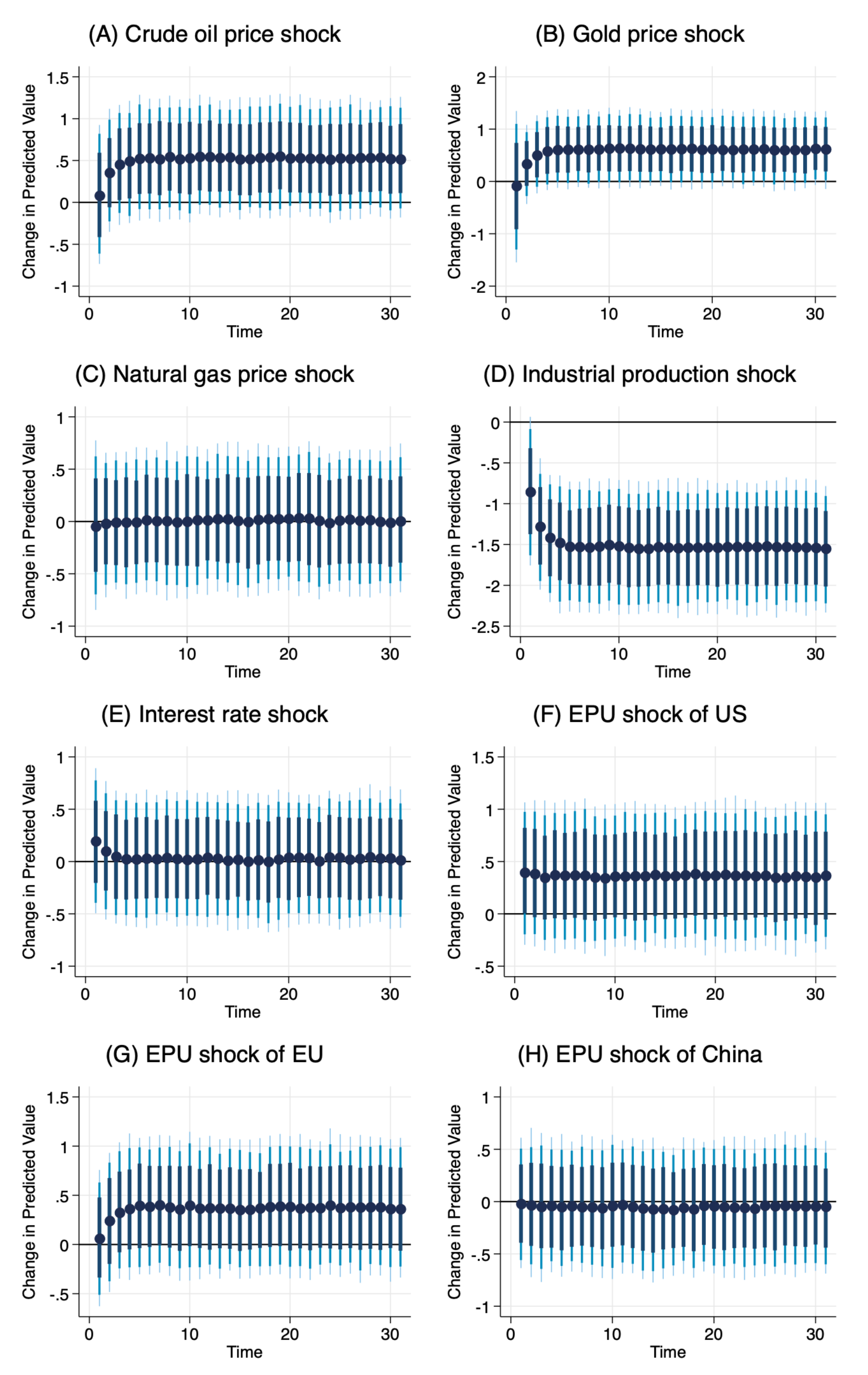
Figure 1A–H depicts the response of Indian economic policy uncertainty to a +1 shock (change) in commodity prices (crude oil, gold, and natural gas prices), industrial production, interest rates, and economic policy uncertainty series (Indian, US, European, and Chinese EPUs) over a 40-month period. Figure 1A, C show that a positive shock to crude oil prices and gold prices, respectively, increases the Indian EPU. This implies that, when there is an increase in crude oil and gold prices, probably due to supply or demand shock, the economic policy uncertainty of India rises significantly. Notably, the effect of gold price changes on the Indian EPU is greater than the effect of crude oil price changes.

Figure 1C indicates that the Indian EPU shows almost no response to shocks in natural gas prices. Conversely, a positive shock to industrial production reduces the Indian EPU throughout the scenario period without reverting to zero. This is demonstrated in Figure 1D. Similarly, as Figure 1E shows, the effect of the interest rate shocks on the Indian EPU is positive but stabilizes in two months’ time. As Figure 1F,G demonstrate, positive shocks in the US and European economic policy uncertainty positively and significantly spillover to Indian economic policy uncertainty, while there is a small but negative spillover from the Chinese economic policy uncertainty, which is displayed in Figure 1H.

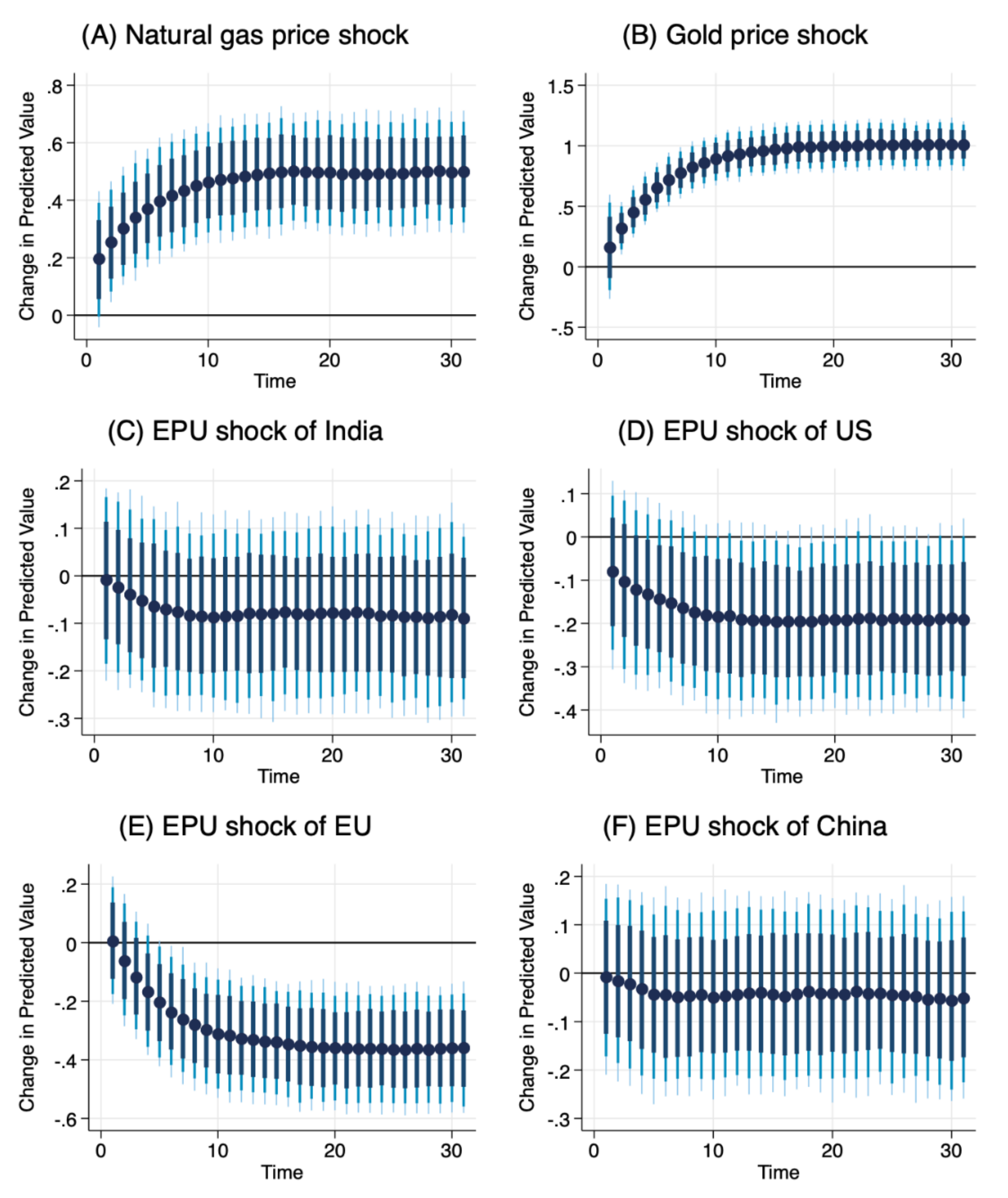
Moreover, Figure 2A–F displays the response of crude oil prices to a positive unit shock (change) on natural gas prices (A), gold prices (B), Indian EPU (C), US EPU (D), European EPU (D), and Chinese EPU (F) for a forty-month scenario period. The plots show that crude oil prices respond positively to a positive shock in natural gas and gold prices. Crude oil prices respond negatively to all EPU shocks. However, the effect of gold is enormous. This confirms the results of the dynamic simulated ARDL presented in Table 4.

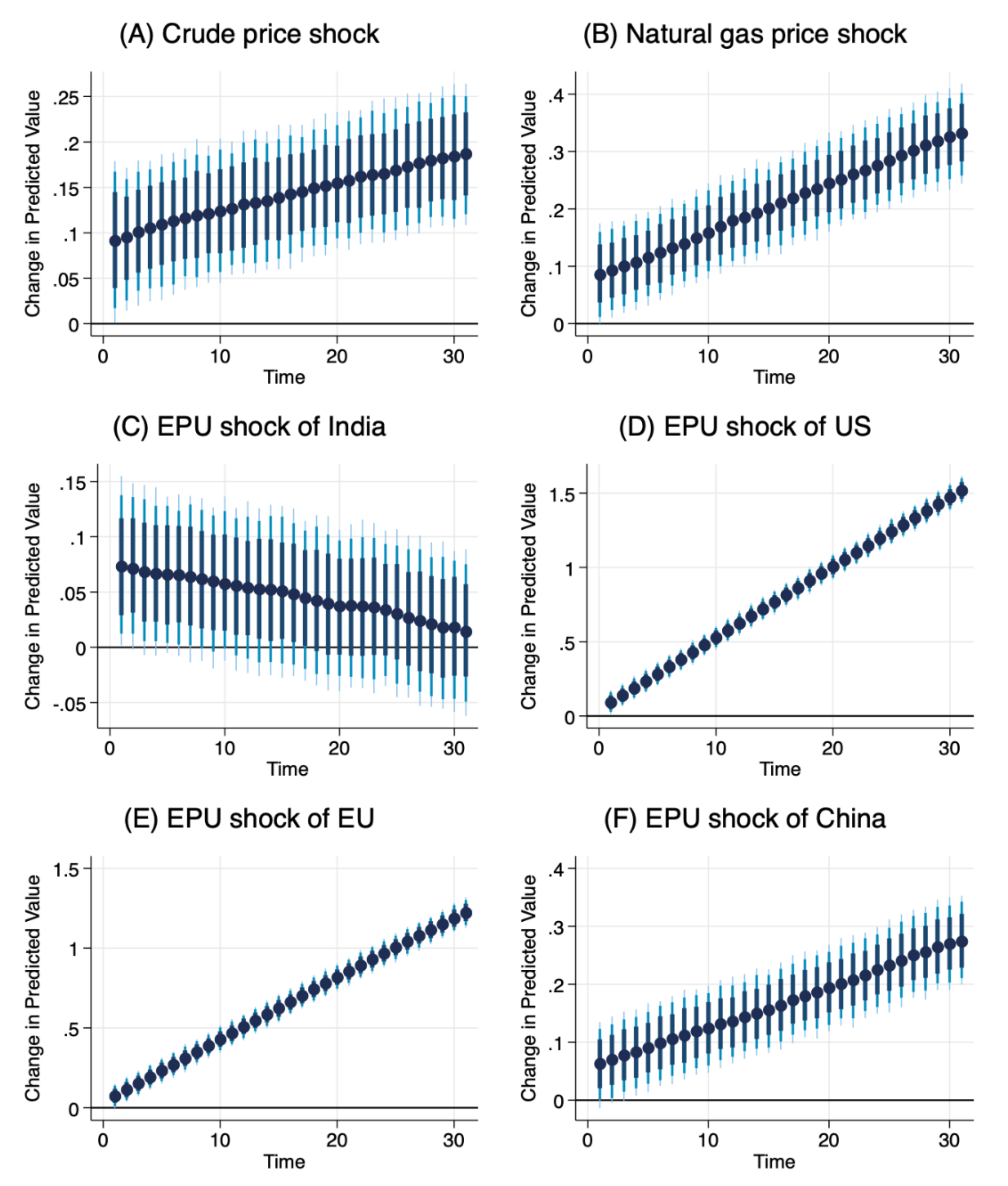
Figure 3A–F depicts the graphical plot for the impulse response representing Model 3 with the gold price as the dependent variable. The plots display the instability (non-convergence) of the model, as indicated by the negative but very close to zero speed of adjustment coefficient estimate in the third column of Table 4. It demonstrates that gold price responds positively and explosively to all positive shocks on all the variables except positive shock on the Indian EPU for which the response dies out slowly. However, the result of the entire model is statistically insignificant, and the graphical exposition is unreliable. This only shows the exogeneity of the gold price in the model.

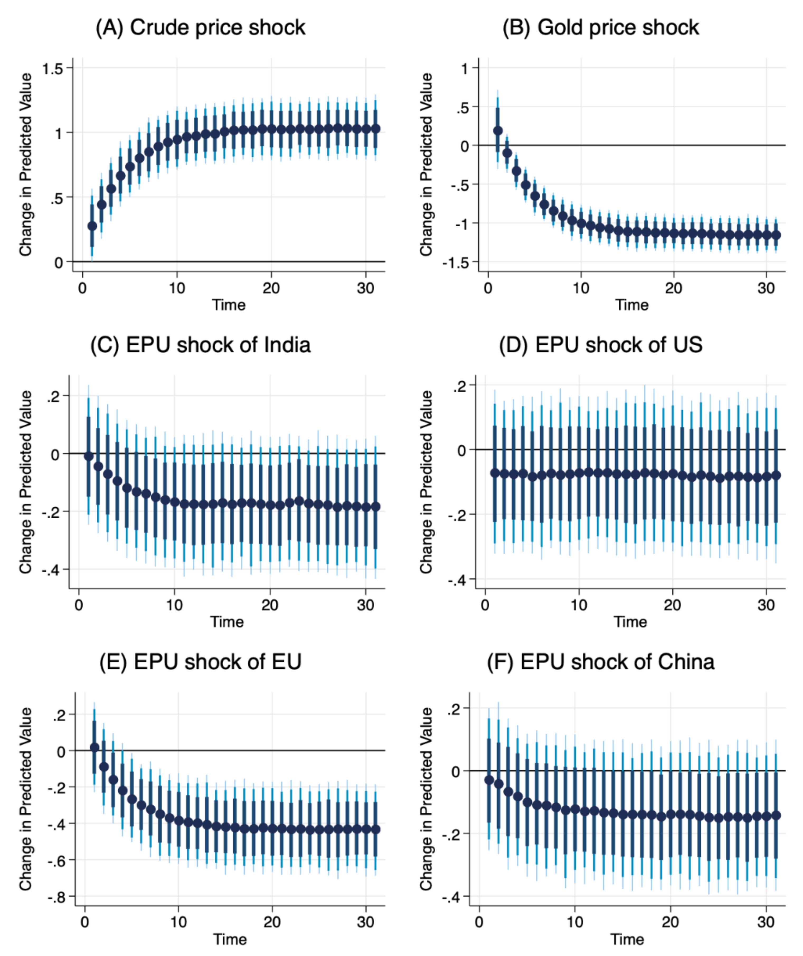
Lastly, Figure 4A–F displays the impulse-response plots of Model 4 in which natural gas price is the dependent variable. The graph displays the response of the natural gas price to counterfactual changes in the EPU series, crude oil prices, and gold prices. It shows that positive shocks to gold prices and EPUs have negative effects on natural gas prices. The response of the natural gas price to a positive shock in crude oil prices is positive, implying that both of these energy prices are driven by the same factors. The effects of the gold and oil price shocks are enormous, while natural gas prices respond negligibly to EPU shocks. Natural gas prices respond positively to positive shocks in crude oil prices. This occurs because of the interconnectedness of the supply of crude oil and natural gas across the world. A supply glut or shortage in crude oil most often leads to the same in natural gas supply. Hence, the prices move concurrently.

5. Conclusions

India is the third largest crude oil consumer, the fourth largest importer of gold, and the fourteenth largest importer of natural gas in the world. Consequently, the high levels of economic policy uncertainty in India might not be unconnected with the instabilities in the prices of these commodities. Hence, examining the interconnections between these variables, as done in this study, is essential for the formulation and implementation of viable economic policies in India. The Indian economy is one of the fastest growing major consumers of all three commodities, and economic policy uncertainty has been a major focus of researchers, investors, and policymakers across the world in recent years. As India is well integrated into the world, economic policy uncertainty shocks in the major world economies might spillover to Indian economic uncertainty. Thus, this study examines the dynamic association between Indian economic policy uncertainty, commodity prices (gold, crude oil, and natural gas), and the economic policy uncertainties of the major world economies (US, Europe, and China) using dynamic simulated ARDL models. Although several studies examined the nexus between economic policy uncertainty and many macroeconomic variables, none considered the interconnections between Indian economic policy uncertainty and the prices of commodities such as crude oil, gold, and natural gas. In particular, none of the studies (also deleted) considered the interaction of the Indian EPU in combination with commodity prices and economic policy uncertainty of the major world economies.

The current study shows that, in the short run, only the industrial production economic policy uncertainty of the US matters for the fluctuations of the Indian economic policy uncertainty. In the long run, crude oil prices, gold prices, industrial production, the US EPU, and European EPU have a significant impact on the Indian EPU. The probable reason for the effect of gold could be the fact that India is a major (4th world largest) consumer of gold, which investors often use as a safe haven to store value during economic turmoil. So, when the price of gold is higher, investors might not be able to buy it, and it loses its hedging or safe haven role. This escalates the economic policy uncertainty in the country. The only saving grace would be an increase in industrial production, which mitigates the effects of the Indian economic policy uncertainty. We also find a significant positive interconnection between gold prices and crude oil prices. The significant positive impact of natural gas prices on crude oil prices manifests both in the short run and the long run. Moreover, changes in crude oil and gold prices significantly affect natural gas prices. Higher crude oil prices are associated with higher natural gas prices and vice versa. On the other hand, higher gold prices significantly reduce the natural gas price and vice versa. The Indian EPU does not have a significant impact on the dynamics of global commodity prices. India is an importer of the commodities and thus has less market power because the effects of supply shocks outweigh the effects of demand shocks in the global market for the commodities. We find significant effects from the US and European economic policy uncertainty on the Indian economic policy uncertainty. The graphical plots further display a great deal of dynamics among the variables. Therefore, the major findings of this study show that, although complex dynamic relationships exist between the Indian macroeconomic variables, crude oil prices, gold prices, industrial production, and the EPUs of the US and Europe are the main channels through which economic policy uncertainty can be influenced in India. Put differently, crude oil prices, gold prices, industrial production, and the EPUs of the US and Europe are the fundamental drivers of Indian economic policy uncertainty. Policymakers in India should consider these factors in shaping the country’s macroeconomic policy. The Indian economic policy uncertainty does not respond to interest rate changes, a major monetary policy tool. Thus, the Central Bank of India’s policy rate changes were not an effective means of controlling the economic policy uncertainty in the country. Policymakers should develop appropriate counter-effective policy tools that have the ability to offset the effects of external forces such as the changes in crude oil prices, gold prices, and the EPUs of the US and Europe.