Two-Level Monitoring System for Preventing Academic Failure, Based on Predictive Models and SHAP Analysis

Abstract

Student dropout remains a critical challenge in higher education, requiring early detection and targeted intervention. This study aims to develop an interpretable two-level monitoring framework for identifying at-risk students—those with academic debts but not yet dismissed—across successive stages of the academic debt lifecycle. Using digital profile data and LMS digital footprints from a large public university (18,192 records covering the years 2022–2024), we trained CatBoost, XGBoost, LightGBM, and Random Forest for each of two stages: initial retakes and final commission retakes. SHapley Additive exPlanations (SHAP) were applied for post hoc interpretation. SHAP analysis identified key indicators of initial retake failure: semester, year of study, number of academic debts, GPA in the previous semester, and LMS activity in the previous and current semesters. The strongest indicator of success on commissions was the presence of a digital footprint at the beginning of the current semester, which eliminated dropout risk regardless of prior academic history. Dismissal risk increases for junior-year students and those with higher debt counts. These findings enabled student profiling into Red, Yellow, and Green risk categories for optimized allocation of administrative and tutoring resources. Utilizing the proposed framework, educators can streamline pedagogical support and enhance student retention.

1. Introduction

Student dropout remains one of the most pressing challenges for higher education institutions worldwide, driving growing research interest in identifying indicators associated with an elevated risk of attrition. Early detection of at-risk students is crucial, since timely and targeted support from university academic and administrative staff can significantly reduce the costs associated with non-completion (Carballo-Mendívil et al., 2025; Chung & Lee, 2019). The drivers of student dropout are heterogeneous, encompassing academic performance, financial difficulties, digital engagement, as well as psychosocial aspects; this complexity often complicates the identification of such students and the organization of effective support.

To address the challenge of detecting at-risk students, machine learning methods are increasingly employed within the field of Learning Analytics (LA). A substantial body of research is dedicated to developing predictive models of academic performance across diverse learning environments, supported by comprehensive systematic reviews such as those by Batool et al. (2023), Namoun and Alshanqiti (2020), and Sghir et al. (2023).

One of the prominent tools of LA exploring predictive models is Early Warning Systems, which leverage student data and predictive modeling to identify learners at risk of failure (Abouelnour et al., 2024; Bañeres et al., 2020). These systems are most frequently built upon complex, often “black-box” predictive models due to their superior predictive accuracy. Ensemble methods, such as Random Forest and XGBoost, demonstrate robust predictive performance in various institutional contexts, often achieving AUC-ROC above 0.90 and accuracy exceeding 90% (Pérez et al., 2025; Bettahi et al., 2025). These models utilize heterogeneous data sources including pre-enrollment characteristics, for example, demographic data and academic indicators from prior education levels, academic records from the current stage of study, behavioral data from digital learning environments, and socio-economic indicators (Dahiya et al., 2025; Borges et al., 2025; Krueger et al., 2023).

Despite advances in LA for solving the dropout prediction task, a significant limitation persists regarding model interpretability. High-performing black-box models, such as neural networks and gradient boosting, provide dropout risk assessment without revealing the underlining factors driving individual predictions. This opacity undermines trust among educators and limits the practical utility of these findings for educational decision-making (Kemper et al., 2020). Achieving a balance between predictive accuracy and explanatory power remains an open challenge. Furthermore, binary risk classification alone is often insufficient to capture the heterogeneous nature of student struggles, necessitating approaches that can uncover underlying patterns of engagement and performance (Wang & He, 2025; Kim et al., 2023).

Many studies employ clustering methods to identify patterns of engagement in the educational process, strategies for interacting with electronic learning resources, and learning styles, as well as the relationship of these patterns with academic success (Le Quy et al., 2023; Palani et al., 2021; Mohamed Nafuri et al., 2022). As an unsupervised technique, clustering eliminates the need for pre-labeled data, enabling immediate pedagogical intervention with current students rather than future cohorts. However, most algorithms—particularly when applied to high-dimensional data—often function as “black boxes”, complicating the interpretability of specific cluster assignments.

Explainable Artificial Intelligence (XAI) addresses the interpretability gap common to both clustering and complex supervised learning models. A typical XAI workflow involves training various predictive models, followed by the application of post hoc explanation methods such as Local Interpretable Model-agnostic Explanations (LIME), Shapley Additive exPlanations (SHAP), or Counterfactual Explanations.

LIME (Ribeiro et al., 2016) focuses on local interpretability, explaining individual predictions by approximating a complex model with simpler, interpretable one in the neighborhood of a specific instance. Conversely, SHAP (Lundberg & Lee, 2017) explains both individual predictions and the overall model behavior, aggregating local contributions into feature importance metrics and summary plots. In LA research these techniques are often used independently—for example, Chen et al. (2022), Sghir et al. (2023), and Pei and Xing (2022) employ LIME to focus on local attribution for specific student outcomes, while Ujkani et al. (2024) and Jang et al. (2022) apply SHAP to identify the primary drivers factors of academic failure. Studies such as da Conceicão Silva et al. (2025), Swamy et al. (2022), Alwarthan et al. (2022), Li et al. (2024) utilize both techniques, allowing for comparison of explanations and assessment of their consistency.

Diverse Counterfactual Explanations (DiCE) (Mothilal et al., 2020) describe the smallest possible change to the initial instance required to yield a different model prediction. Swamy et al. (2022), Afrin et al. (2023), and Buñay-Guisñan et al. (2025) apply DiCE to explain student success prediction models and generate individual or group counterfactuals. Based on these counterfactuals actionable plans can be developed to help at-risk students transition from predicted failure to academic success.

Notably, most research focuses on predicting dropout or course failure (i.e., the initial occurrence of academic debts). However, between the initial failure of an exam and final dismissal, a student traverses several distinct stages (e.g., retake attempts). These stages represent critical windows where the most intensive and personalized pedagogical intervention should be implemented, meaning that predictive analytics of students’ performance and engagement during these specific phases hold significant promise. Despite this, insufficient attention has been paid to this in LA literature to date.

In this study, we utilize educational data from a large Russian university—Siberian Federal University (SibFU)—and focus primarily on at-risk students: those who have accrued academic debts but have not yet been dismissed.

The objectives of this research are as follows:

RA1: To develop a framework for monitoring at-risk students that accounts for the distinct stages of the academic cycle, based on a combination of predictive analytics and XAI.

RA2: To develop and evaluate predictive models for the stage-by-stage forecasting of academic failure among at-risk students at SibFU.

RA3: To establish a set of interpretable indicators of academic failure, and to profile student groups with varying risk levels based on XAI analysis results.

2. Materials and Methods

2.1. Dismissal Regulations

In accordance with Federal Law No. 273-FZ “On Education in the Russian Federation” (Russian Federation, 2012), two types of termination of educational relations are distinguished: successful completion of studies and early termination, i.e., dropout. Dropout occurs when a student is unable or unwilling to continue their education for various reasons. Early termination may be initiated either by the student (voluntary withdrawal) or by the educational organization—due to academic failure, non-payment of tuition, violation of the organization’s charter, and other grounds. In the context of this study, “dropout” refers specifically to academic dropout—early termination initiated by the organization due to academic failure. This specific type follows a formalized administrative trajectory, making it highly suitable for predictive modeling.

In accordance with the Law (Russian Federation, 2012), students who receive unsatisfactory results during an intermediate assessment are granted the opportunity to rectify their academic debt. The educational institution is prohibited from dismissing a student immediately after the occurrence of academic debt; instead, the student is granted no more than two retake attempts within one year. The specific deadlines and procedural details for these retakes are governed by the university’s internal regulatory acts.

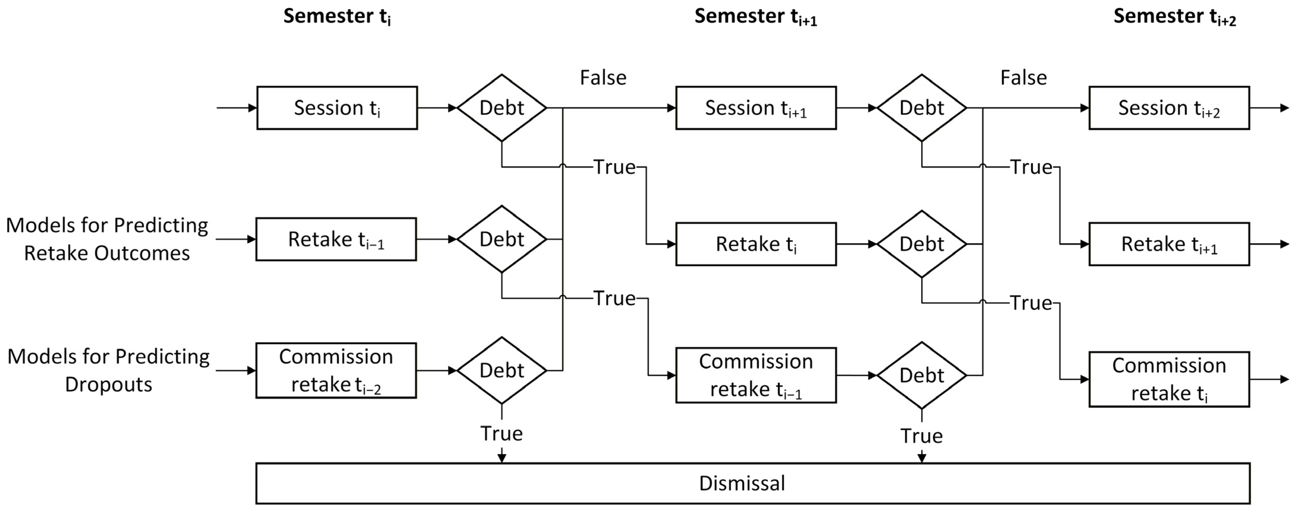
At SibFU, the following regulations are applied (Figure 1): when academic debt occurs in semester $t_i$, the student is granted the right to a first retake during semester $t_{i+1}$. Following an unsuccessful attempt, a final commission retake is scheduled within semester $t_{i+2}$. The commission is composed of the course examiner and two additional faculty members with relevant expertise. Students who fail to eliminate academic debt within the established timeframe are dismissed for failure to fulfill the curriculum requirements (Siberian Federal University, 2023).

To formally describe this process and formulate the machine learning task, we introduce the following notation. Let $S=\left\{s_1,s_2,\dots ,s_N\right\}$ be the set of students, $D=\left\{d_1,d_2,\dots ,d_M\right\}$ be the set of disciplines in the curriculum, and $T=\left\{t_1,t_2,\dots ,\right\}$ be a discrete timeline of semesters, where $t_i$ denotes the $i$-th semester of study. For a student $s\in S$ in semester $t_i$, we define $L\left(s,t_i\right)\subseteq D$ as the set of disciplines for which the student $s$ has academic debt at the end of semester $t_i$.

$$L\left(s,t_{i+1}\right)=\left(L\left(s,t_i\right)\backslash C\left(s,t_i\right)\right)\cup F\left(s,t_i\right),$$

where $C\left(s,t_i\right)\subseteq L\left(s,t_i\right)$ is the set of debts eliminated in semester $t_i$, and $F\left(s,t_i\right)\subseteq D$ is the set of disciplines failed in the final assessment of semester $t_i$.

Student $s$ is dismissed for academic failure in semester $t_{i+2}$ if after two retake attempts (initial retake and commission retake), they fail to eliminate at least one academic debt incurred in the $i$-th semester:

$$\exists d\in D:d\in F\left(s,t_i\right)\wedge d\notin C\left(s,t_{i+1}\right)\wedge d\notin C\left(s,t_{i+2}\right).$$

Thus, the maximum number of attempts to pass discipline $d$ is three: the primary examination session in semester $t_i$, an initial retake in semester $t_{i+1}$, and a final commission retake in semester $t_{i+2}$. Students who fail the third attempt are subject to dismissal.

Based on this procedure, a two-level academic failure monitoring system was developed at the university. The system architecture and characteristics of the models employed are presented in

Table 1. Characteristics of the predictive models for academic failure monitoring system.

Model	Semester	Features	Target	$\mathit{F}1$-Score
Models for Predicting Retake Outcomes	$t_{i+1}$	$X_{risk}\left(s,t_{i+1}\right)$	Retake Failure	0.75
Models for Predicting Dropouts	$t_{i+2}$	$X_{risk}\left(s,t_{i+2}\right)$	Dropout	0.85

.

In Table 1, $X_{risk}\left(s,t_{i+1}\right)$ and $X_{risk}\left(s,t_{i+2}\right)$ are aggregated student digital footprint and digital profile data associated with retake outcomes, collected up to and including the $t_{i+1}$ ($t_{i+2}$) semester, respectively.

The Level-1 Model is designed to predict the outcome of the first retake in semester $t_{i+1}$. The target variable for this model is a binary feature: “unsuccessful attempt to eliminate academic debts from semester examination session $t_i$”. This level serves as an early intervention point, enabling preventive support before the student reaches the final commission retake stage.

The Level-2 Model is the dropout prediction model, activated at the commission retake stage in semester $t_{i+2}$. The target variable corresponds to the failure to eliminate academic debts within the established timeframe which, according to institutional regulations, triggers the dismissal procedure. This level provides high-stakes decision support for retention interventions.

To ensure interpretability of predictions at both levels—which represent critical decision points for student retention—the XAI method SHAP is employed. The use of SHAP facilitates the analysis of “black box” model predictions by identifying essential risk factors and behavioral patterns affecting the probability of the unsuccessful retake or dropout, thereby enabling tutors and administrators to apply targeted preventive measures.

2.2. Educational Data

In this study, we utilize two types of educational data: student digital profiles and digital footprints from Learning Management System (LMS). In previous research (Kustitskaya et al., 2023, 2025), based on data extracted from various university electronic services between the 2018 and 2024 academic years, we formed two datasets and described them in detail—the Digital Profile Dataset and the Digital Footprint Dataset.

The Digital Profile Dataset provides a digital personal portrait of students and their prior educational history. This includes demographic data, information on their current curriculum and degree programs, a history of academic status changes (transfers between academic programs, academic leaves, academic dropout, and reinstatements), and student grade book data.

The Digital Footprint Dataset comprises data on students’ educational behavior and performance extracted weekly from the university’s Moodle-based e-learning platform, “e-Courses”. It includes detailed information on students’ interactions with e-course materials and their corresponding scores within the e-course gradebooks.

Both datasets were utilized to develop models predicting academic success at the conclusion of the semester. Success is defined as passing all curriculum courses within the semester, while failure is defined as failing at least one course, resulting in one or more academic debts. These models were originally presented in Kustitskaya et al. (2024) and are currently embedded into the academic performance forecasting service, Pythia (https://services-sfu.ru/pifiya, accessed on 15 April 2026).

However, these datasets also contain data that can provide valuable insights into the specific characteristics of a student’s subsequent educational behavior following the occurrence of academic debt. Furthermore, they highlight features within student educational profiles that are associated with an increased risk of repeated failure and academic dropout.

To analyze the preconditions for failure to eliminate academic debts, we extracted information from both the Digital Profile Dataset and the Digital Footprint Dataset for students who incurred at least one debt following an examination session. From this group, we specifically identified individuals for whom LMS digital footprint data was available both for the semester in which the debt originated and for the subsequent semester during which retakes occurred.

As a result, we obtained a dataset comprising educational profile and LMS digital footprint data for students with academic debts. The dataset covers the 2022–2023 and the 2023–2024 academic years and contains 18,192 records. The anonymized data is available at [https://github.com/TaK-analytics/XAI-for-academic-failure-prediction (accessed on 5 April 2026)].

The majority of students successfully passed their initial retakes. Consequently, the task of identifying the preconditions for dropout was focused exclusively on the subset of students who failed the first retake attempts. Accordingly, the dataset was filtered to 6387 records for this specific task.

2.3. Level-1 Models—Models for Predicting Retake Outcomes

To examine the relationship between the characteristics of students’ educational profiles, their digital learning behavior, and the risk of failing the first retake, a binary classification task was performed. The binary response variable, Retake Failure, was set to ‘1’ if a student retained at least one unresolved academic debt after the initial retake period, and ‘0’ otherwise.

2.3.1. Algorithm Selection and Model Complexity Calibration

Prior to the main modeling phase, a systematic pilot screening was conducted to identify the most suitable algorithms for the educational dataset. A broad pool of models—including single decision trees, LASSO-regularized logistic regression, Random Forest, XGBoost, CatBoost, LightGBM, and various neural network architectures—was evaluated. The dataset was split into training and test subsets in a 70:30 ratio. For the initial baseline assessment, tree-based ensembles, linear models, and single decision trees were fitted using 5-fold cross-validation on the training set. All models were implemented with default hyperparameters using scikit-learn 1.7.2, XGBoost 3.0.1, CatBoost 1.2.8, and LightGBM 4.6.0. These defaults represent well-established, robust starting points that balance computational efficiency and generalization across benchmark datasets, making them suitable for rapid initial screening. Models falling below a predefined baseline threshold (F1-score < 0.70) in this phase were excluded from further development. Consequently, the single decision tree and LASSO-regularized logistic regression were discarded due to their subpar predictive performance (average F1-score = 0.65 and average F1-score = 0.64, respectively).

The remaining tree-based ensembles and neural networks proceeded to hyperparameter optimization via 5-fold cross-validation. For neural networks, we evaluated both fully connected architectures and architectures incorporating one-dimensional convolutional blocks to capture temporal patterns in digital footprint sequences. Approximately 1000 configurations were tested, varying network depth, batch size, optimizer, learning rate, focal loss weighting, oversampling strategy, and decision thresholds. The best-performing neural network achieved an F1-score of 0.69 on the test set, which remained below the performance of the tuned tree ensembles. Therefore, the subsequent analysis and SHAP-based interpretation focused exclusively on Random Forest, XGBoost, CatBoost, and LightGBM.

As significant overfitting was observed for these models despite hyperparameter tuning, we implemented a procedure to identify the specific complexity thresholds beyond which model generalization begins to degrade. Guided by CatBoost Documentation (n.d.), XGBoost Documentation (n.d.), LightGBM Documentation (n.d.), and Scikit-Learn Documentation (n.d.), we identified the specific hyperparameters governing model complexity.

To establish empirical limits for these parameters, we isolated each hyperparameter for investigation (denoted as H) while exploring the remaining parameters via a GridSearch procedure. For each unique combination of the remaining hyperparameters, we iterated through a range of values for H. At each step, we utilized 5-fold cross-validation to compute the average F1-score across training folds, the average F1-score across test folds, and the resulting gap between them. For each specific hyperparameter H, we identified the value at which the first significant increase in the gap size occurred, signaling the onset of overfitting. After traversing the entire search grid for H, we collected these identified points and calculated their median value. We defined this median as the threshold for H beyond which the model would incur a penalty for excessive complexity in our subsequent optimization framework. We obtained the following thresholds:

• for CatBoost: “iterations” larger than 800, “max_depth” larger than 8, “learning_rate” larger than 0.1, “l2_leaf_reg” less than 5, “border_count” less than 64, “random_strength” less than 1.5;
• for XGBoost: “n_estimators” larger than 500, “max_depth” larger than 5, “learning_rate” larger than 0.1, “reg_lamda” less than 5, “reg_alpha” less than 1, “subsample” less than 0.8, “colsample_bytree” less than 0.8, “gamma” less than 1;
• for RandomForest: “n_estimators” larger than 200, “max_depth” larger than 10, “min_samples_split” less than 5, “min_samples_leaf” less than 3, “max_samples” less than 0.8;
• for LightGBM: “n_estimators” larger than 1000, “max_depth” larger than 6, “learning_rate” larger than 0.1, “reg_lambda” and “reg_alpha” less than 1, “num_leaves” larger than 50, “subsample” less than 0.8, “colsample_bytree” less than 0.8.

The primary limitation of this empirical approach is that it evaluates complexity-controlling hyperparameters in isolation. As a result, univariate median thresholds may not fully capture regions where multiple parameters interact to cause overfitting. However, these thresholds are not used to restrict the search space, but rather to introduce a penalty term into the objective function during the selection process described below.

2.3.2. Integrated Model Optimization and Feature Selection

At the next stage of the modeling process, we performed simultaneous hyperparameter optimization and feature selection for all remaining models using a 5-fold nested cross-validation procedure. This approach was designed to achieve several key objectives:

• feature space reduction to select a more compact subset of predictors and enhance model interpretability;
• overfitting mitigation;
• performance maximization to the greatest extent possible while maintaining model parsimony.

In each iteration of the inner loop of the nested cross-validation, the tuning of the optimal hyperparameters was performed utilizing the Bayesian optimization technique (specifically, the Tree of Parzen Estimators algorithm). The objective function for minimization was the following:

$$\mathrm{L}\left(\mathrm{h}\mathrm{y}\mathrm{p}\mathrm{e}\mathrm{r}\mathrm{p}\mathrm{a}\mathrm{r}\mathrm{a}\mathrm{m}\mathrm{s}\right)=1-\mathrm{F}1\mathrm{s}\mathrm{c}\mathrm{o}\mathrm{r}\mathrm{e}\left(\mathrm{h}\mathrm{y}\mathrm{p}\mathrm{e}\mathrm{r}\mathrm{p}\mathrm{a}\mathrm{r}\mathrm{a}\mathrm{m}\mathrm{s}\right)+\mathrm{p}\mathrm{e}\mathrm{n}\mathrm{a}\mathrm{l}\mathrm{t}\mathrm{y}\left(\mathrm{h}\mathrm{y}\mathrm{p}\mathrm{e}\mathrm{r}\mathrm{p}\mathrm{a}\mathrm{r}\mathrm{a}\mathrm{m}\mathrm{s}\right),$$

where penalty(hyperparams) penalizes model complexity using the thresholds described in Section 2.3.1.

Within each iteration of the Bayesian optimization process, stepwise forward feature selection was conducted based on an Akaike Information Criterion-like (AIC-like) penalty:

$${\mathrm{A}\mathrm{I}\mathrm{C}\text{-}\mathrm{l}\mathrm{i}\mathrm{k}\mathrm{e}=2\mathrm{k}+2\mathrm{N}}_{\mathrm{t}\mathrm{r}\mathrm{a}\mathrm{i}\mathrm{n}}·\mathrm{L}\mathrm{o}\mathrm{g}\hspace{0.17em}\mathrm{L}\mathrm{o}\mathrm{s}\mathrm{s}\left(\mathrm{t}\mathrm{r}\mathrm{a}\mathrm{i}\mathrm{n}\right),$$

where k refers to the number of predictors, ${\mathrm{N}}_{\mathrm{t}\mathrm{r}\mathrm{a}\mathrm{i}\mathrm{n}}$ is the size of the training fold, and Log Loss(train) is the binary classification metric Log Loss computed on the training fold.

In the outer loop of the nested cross-validation, the resulting model for each iteration was evaluated on the respective test fold.

Table 2. Comparative performance and complexity of classification models for predicting retake outcomes: baseline vs. optimized configurations (the best-performing model is highlighted).

Before the integrated hyperparameter tuning and feature selection
	Accuracy, precision, recall, F1-score
	CatBoost	XGBoost	LightGBM	Random Forest
on the train dataset	0.872, 0.845, 0.804, 0.824	0.900, 0.796, 0.985, 0.880	0.850, 0.819, 0.767, 0.792	0.922, 0.915, 0.871, 0.893
on the test dataset	0.822, 0.773, 0.738, 0.755	0.756, 0.678, 0.860, 0.758	0.819, 0.772, 0.729, 0.750	0.814, 0.759, 0.733, 0.746
number of predictors	58	58	58	58
After the integrated hyperparameter tuning and feature selection
on the train dataset	0.834, 0.806, 0.787, 0.796	0.824, 0.762, 0.773, 0.767	0.854, 0.829, 0.814, 0.821	0.839, 0.800, 0.812, 0.806
on the test dataset	0.820, 0.760, 0.759, 0.759	0.816, 0.754, 0.755, 0.754	0.816, 0.751, 0.758, 0.755	0.808, 0.732, 0.767, 0.749
number of predictors	20	21	27	24

presents a comparative analysis of model performance on the training and held-out test datasets, both before and after the integrated optimization and feature selection process. While the best-performing model is highlighted, it should be noted that all four models demonstrate comparable performance levels.

It is evident that while the predictive quality on the test dataset remains virtually unchanged, the resulting models are substantially more compact in terms of the number of predictors.

In our study, we employed the integrated design with an AIC-like criterion to directly balance model fit and parsimony. However, alternative strategies for feature space reduction in tree-based ensembles, including permutation importance, recursive feature elimination, and SHAP-based selection, are well-established options that could also be considered for this task.

Table 3. Comparative analysis of predictor sets and their feature importance in optimized models for retake outcomes prediction (the highest importance scores for each model are highlighted).

Predictors	Feature Importance for Models
	CatBoost	XGBoost	LightGBM	Random Forest
Number of academic debts in previous semester	0.181	0.184	0.189	0.213
Semester_Spring	0.175	0.166	0.204	0.152
Year_2023	0.063	0.069	0.049	0.075
Number of active clicks at week 18 of the previous semester (z-scaled)	0.013	-	0.037	0.003
Number of academic debts after first retakes (two semesters prior)	0.010	0.007	0.012	0.005
GPA after second retakes (two semesters prior)	0.008	-	-	0.011
School_13	0.008	0.008	0.007	0.004
Average grade for all e-courses at week 18 of the previous semester (z-scaled)	0.007	0.008	0.003	0.001
Year of study	0.007	0.015	0.017	0.002
School_16	0.006	0.007	0.007	0.005
Number of academic debts from two semesters prior	0.005	0.008	0.006	0.002
GPA in the previous semester	0.004	0.003	0.007	0.002
Average grade for all e-courses at week 7 of the current semester (z-scaled)	0.004	-	0.005	-
Number of active clicks at week 7 of the current semester (z-scaled)	0.004	0.005	0.002	0.001
School_4	0.004	0.001	0.002	-
Age	0.002	-	0.002	0.001
Downtime at week 4 of the current semester	0.002	0.002	0.002	0.001
Downtime at week 7 of the current semester	0.002	-	-	-
School_1	0.001	0.000	0.001	0.003
Number of effective clicks at week 18 of the previous semester (z-scaled)	0.001	-	-	0.001
Number of active clicks at week 10 of the previous semester (z-scaled)	-	0.003	-	-
Level of academic program_Specialist	-	0.003	0.004	-
School_7	-	0.003	0.004	-
School_3	-	0.001	-	-
School_18	-	0.000	-	-
School_23	-	0.000	-	-
School_22	-	0.000	-	-
Number of active clicks at week 4 of the current semester (z-scaled)	-	-	0.007	0.002
Average grade for all e-courses at week 7 of the current semester (z-scaled)	-	-	0.005	0.001
Number of effective clicks at week 4 of the current semester (z-scaled)	-	-	0.002	-
Average grade for all e-courses at week 10 of the previous semester (z-scaled)	-	-	0.005	0.000
Number of active clicks at week 10 of the previous semester (z-scaled)	-	-	0.004	-
Number of effective clicks at week 7 of the current semester (z-scaled)	-	-	0.004	0.002
School_10	-	-	0.002	-
Average grade for all e-courses at week 4 of the current semester (z-scaled)	-	-	0.008	0.000
Number of academic debts for graded exams in previous semester	-	-	-	0.001
School_9	-	-	-	0.001

presents the predictor subsets retained after the feature selection process, alongside the feature importance for each predictor. The five features with the highest importance scores for each model are highlighted.

In Table 3, feature importance is calculated via permutation importance on the test dataset using the F1-score as the scoring metric. Notably, the three most influential indicators across all models are Number of academic debts in the previous semester, Semester_Spring, and Year_2023.

Although the presented integrated design was employed for model optimization, alternative strategies for feature space reduction in tree-based ensembles are available, among which permutation importance, recursive feature elimination, and SHAP-based selection represent well-established options that could substitute for the AIC-like criterion used in this study.

2.4. Level-2 Models—Models for Predicting Dropouts

To predict the probability of academic dropout, we utilized the same datasets (the Digital Profile Dataset and the Digital Footprint Dataset), excluding variables that are unavailable at the start of the commission retake period. For instance, when predicting initial retake failure, we employed predictors such as the average grade and the total number of active clicks across all e-courses at week 7 of the current semester. This is feasible because retakes for academic debts from the preceding examination session typically occur after week 8. In contrast, for the dropout prediction task, these predictors cannot be used, because commission retakes for debts from two semesters prior—and the subsequent dropouts—commence as early as week 5 of the semester, a point at which these predictors have not yet become available.

The binary target variable, Dropout, was set to ‘1’ for students who were dismissed following the commission retakes of academic debts incurred two semesters prior, and ‘0’ otherwise.

The approach to classifier selection and training was analogous to that described in Section 2.3, with a minor modification to the integrated model optimization and feature selection procedure. Due to the class imbalance in the dataset (Class 1–17%, Class 0–83%), RandomOverSampler from the “imblearn” library was employed. This oversampling strategy was selected because the feature space consists of 12 ordinal, 32 binary, and 21 continuous features; consequently, 68% of predictors are not continuous. Therefore, the Synthetic Minority Over-sampling Technique (SMOTE) is not suitable in this context. Furthermore, SMOTE-NC, which is designed for mixed datasets, was rejected for methodological reasons. While RandomOverSampler duplicates existing observations—thereby guaranteeing that all feature combinations in the training set remain authentic and logically consistent—SMOTE-NC generates synthetic samples via interpolation. In the educational context, this interpolation can produce synthetic student profiles that represent average patterns rather than actual behavioral patterns, potentially undermining the reliability of subsequent SHAP explanations.

The “sampling_strategy” parameter of RandomOverSampler was optimized within the inner loop of the nested cross-validation framework alongside the model hyperparameters. The parameter was tuned within the range bounded by the original minority ratio (corresponding to no resampling) and 1.0 (corresponding to a balanced 50:50 distribution). The following optimal values were obtained: 0.3 for CatBoost and LightGBM (resulting in a 23.1% minority class share within the training fold), 0.275 for XGBoost (21.6%), and 0.4 for Random Forest (28.6%).

The resulting four models for academic dropout prediction demonstrated superior predictive performance compared to the previously described Level-1 models for retake failure prediction. At the same time, they are more compact, as they utilize a smaller subset of predictors.

Table 4. Comparative performance and complexity of classification models for predicting dropouts: baseline vs. optimized configurations (the best-performing model is highlighted).

Before the integrated hyperparameter tuning, oversampling and feature selection
	Accuracy, precision, recall, F1-score
	CatBoost	XGBoost	LightGBM	Random Forest
on the train dataset	0.997, 0.984, 0.897, 0.939	0.997, 0.962, 0.933, 0.947	0.996, 0.950, 0.895, 0.922	0.996, 0.972, 0.877, 0.922
on the test dataset	0.992, 0.886, 0.793, 0.837	0.992, 0.880, 0.784, 0.829	0.991, 0.880, 0.770, 0.821	0.990, 0.856, 0.746, 0.797
number of predictors	65	65	65	65
After the integrated hyperparameter tuning, oversampling and feature selection
on the train dataset	0.969, 0.922, 0.947, 0.935	0.963, 0.905, 0.926, 0.916	0.963, 0.906, 0.936, 0.921	0.963, 0.920, 0.954, 0.937
on the test dataset	0.961, 0.874, 0.896, 0.885	0.952, 0.836, 0.884, 0.859	0.950, 0.830, 0.877, 0.853	0.946, 0.815, 0.874, 0.844
number of predictors	16	19	15	13

and

Table 5. Comparative analysis of predictor sets and their feature importance in optimized models for dropout prediction (the highest importance scores for each model are highlighted).

Predictors	Feature Importance for Models
	CatBoost	XGBoost	LightGBM	Random Forest
Predictors of the Models and Their Feature Importance
Downtime at week 4 of the current semester	0.410	0.447	0.490	0.505
Number of active clicks at week 4 of the current semester	0.177	-	-	0.000
Number of academic debts in previous semester	0.143	0.081	0.107	0.218
Downtime at week 18 of the previous semester	0.087	0.030	0.021	0.079
Semester_Spring	0.128	0.129	0.130	0.139
Year of study	0.051	0.034	0.029	0.051
Average grade for all e-courses at week 4 of the current semester	0.035	0.053	-	0.000
School_17	0.030	0.029	0.024	0.008
School_2	0.026	0.008	0.005	-
Number of active clicks at week 10 of the previous semester	0.023	0.013	-	-
Year_2023	0.022	-	-	-
Number of effective clicks at week 4 of the current semester	0.019	-	-	0.000
Year_2024	0.018	0.030	0.022	0.023
School_14	0.015	0.016	0.007	-
Number of effective clicks at week 10 of the current semester	0.015	-	-	0.007
School_13	0.012	-	-	-
Funding type_tuition-paying	-	0.017	0.018	0.009
Downtime at week 10 of the previous semester	-	0.017	0.015	-
Number of active clicks at week 18 of the previous semester	-	0.005	0.011	-
Average grade for all e-courses at week 18 of the previous semester	-	0.002	0.003	-
GPA in the previous semester	-	0.002	-	-
Number of academic debts from two semesters prior	-	0.000	0.000	-
School_6	-	0.000	-	-
School_10	-	0.000	-	-
Age	-	-	0.004	-
Number of academic leaves	-	-	-	0.002

present the outcomes of the integrated optimization, oversampling and feature selection processes for the dropout forecasting models.

The CatBoost model demonstrated the best performance, achieving precision = 0.87, recall = 0.90, and an F1-score = 0.89 on the test set. It is also worth noting that the sets of predictors differ considerably across the models, although two predictors—Downtime at week 4 of the current semester, Number of academic debts in the previous semester and Semester_Spring—are consistently ranked among the top five most important features for all four models.

While a single predictive model incorporating time-aware features could theoretically be constructed, we deliberately structured the monitoring system into two sequential levels for three interrelated reasons. First, the institutional retention workflow comprises two distinct decision milestones—initial retakes and commission retakes—each governed by different protocols and intervention timelines. Second, standard tabular machine learning algorithms require a fixed feature matrix; integrating temporally staggered variables into one model would necessitate extensive imputation or dynamic masking, risking temporal leakage and undermining operational transparency. Third, separating the levels preserves stage-specific SHAP interpretability, enabling precise, pedagogically meaningful risk attribution at each decision point without conflating feature contributions across disparate academic phases.

2.5. Explainable AI for Exploring Feature Contributions to Predictions of Machine Learning Models

One of the tools in XAI that allows for the estimation of a variable’s contribution to a machine learning model’s prediction is based on Shapley values. A Shapley value (Shapley, 1953) is a method for allocating payoffs to players depending on their contribution to the total payout.

In a machine learning (ML) context, each predictor is treated as a “player”, and the Shapley values assess its individual contribution to the model’s predicted outcome.

Let f be a prediction model and f(x) be a prediction obtained for a single instance x. Let F be the complete set of all features, and S ⊆ F be a subset of F. To evaluate the impact of including feature j in the model on the model’s prediction, two models are compared: $f_{S\cup \left\{j\right\}}$ which is trained with the feature present, and $f_S$ which is trained with the feature withheld. The Shapley value for feature j is calculated using the formula:

$${\phi }_j=\sum _{S\subseteq F\backslash \left\{j\right\}}{\displaystyle \frac{\left|S\right|!\left(\left|F\right|-\left|S\right|-1\right)!}{\left|F\right|!}}\left(f_{S\cup \left\{j\right\}}(x)-f_S(x)\right).$$

SHAP, introduced in Lundberg and Lee (2017), is a method for explaining individual predictions using SHAP values—specific approximations of Shapley values designed for ML models.

Consider a specific instance x from a background dataset X. Using SHAP values, the model’s prediction f(x) for the instance x can be represented as follows:

$$f\left(x\right)=E\left[f\left(x\right)\right]+\sum _{j\in F}{SHAP}_j,$$

where $E\left[f\left(x\right)\right]$ is the average prediction of the model over dataset X, known as the base value.

As the predictive models used in this case are tree-based, we calculate the SHAP values using TreeSHAP (Lundberg et al., 2020)—an estimator specifically designed for tree-based ML models. To compute SHAP values and visualize their distributions, we utilize the SHAP library (version 0.46.0) for Python (version 3.12.3) (Lundberg & Lee, 2017).

For binary classification tasks the explainers within the SHAP package return SHAP values in log-odds space. To facilitate an intuitive interpretation of predictor effects on the probability of failure (or dropout), we mapped the SHAP values to the probability scale using the sigmoid transformation for specific visualizations.

The contribution of the most significant model variables to the predictions warrants particular attention. To assess the strength of a feature’s influence on the model’s prediction—rather than on tree construction—we employ SHAP feature importance to identify the most influential predictors. For a given feature, this metric is computed as the mean of the absolute SHAP values across the entire sample under analysis.

Although the SHAP analysis could be limited to the best-performing model, we examine all four models to assess the robustness of predictor–prediction relationships across algorithms. Specifically, we seek to determine whether these identified relationships exhibit similar patterns regardless of the underlying model. Accordingly, for each distinct predictive task, we compute, visualize, and analyze the SHAP values for all four models: Random Forest, XGBoost, CatBoost, and LightGBM.

3. Results

3.1. SHAP Analysis for Models Predicting Retake Failures

The analysis of the contributions of various digital profile and digital footprint characteristics to the prediction of retake failure was conducted for all four Level-1 Models presented in Section 2.3. In this subsection, we briefly describe the results obtained. However, the visual SHAP analysis is presented only for the CatBoost model, as it demonstrated slightly higher prediction accuracy than the other models. We first examine the contribution of various predictor variable values to the model’s predictions.

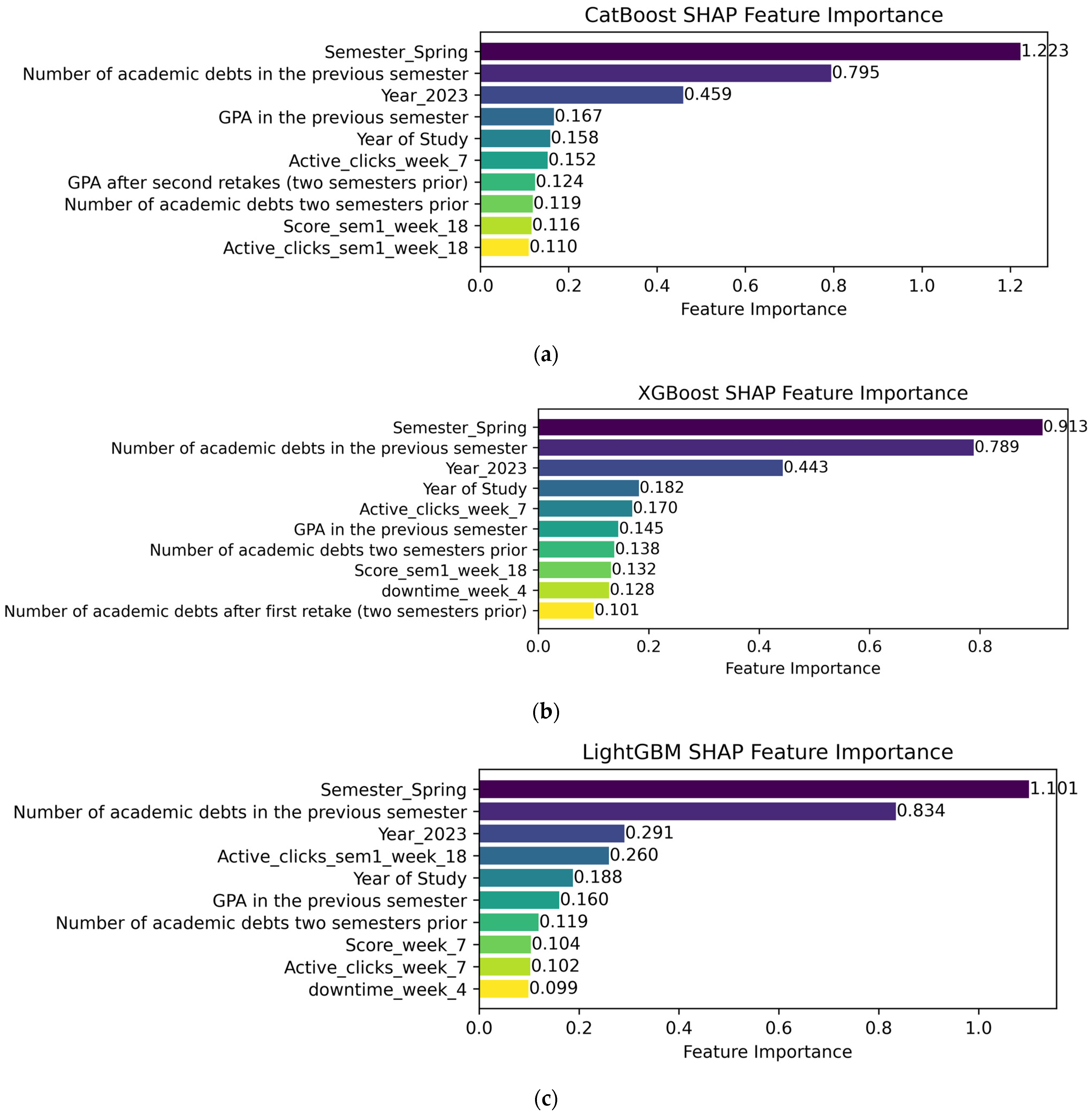
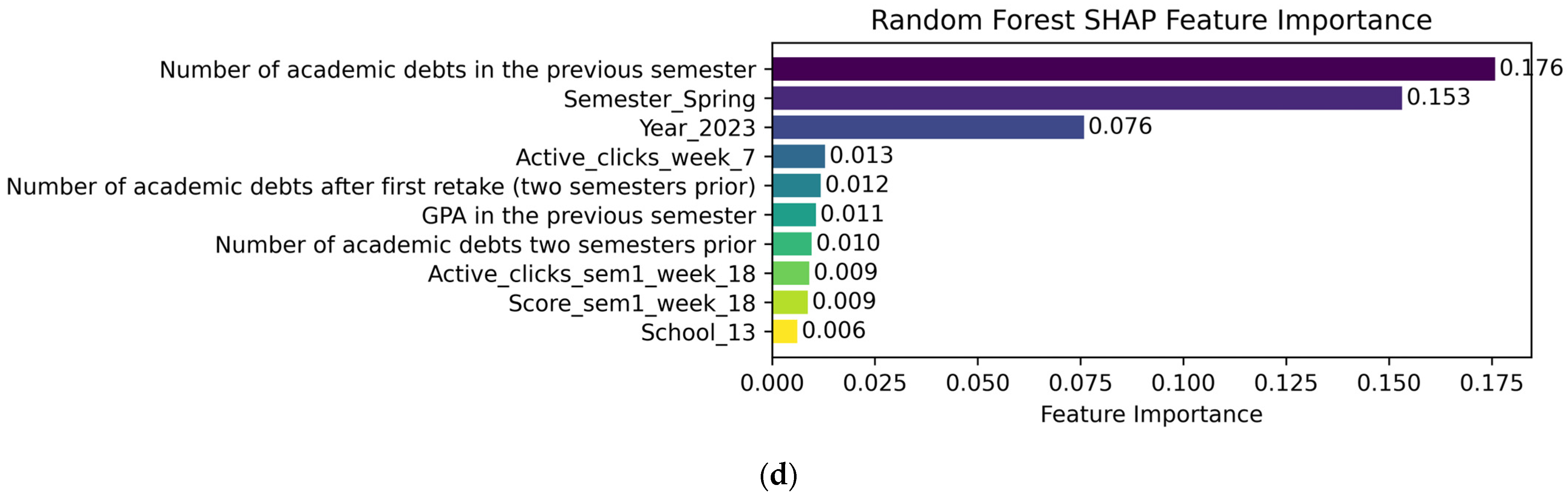
Figure 2 presents a comparative analysis of SHAP feature importances across the four models used to predict retake failures.

We subsequently analyzed the features with the highest SHAP feature importance (as identified in Figure 2) for all four models: Semester_Spring, Year_2023, Number of academic debts in the previous semester, Year of Study, Number of active clicks at week 7 of the current semester, GPA in the previous semester, and Number of active clicks at week 18 of the previous semester.

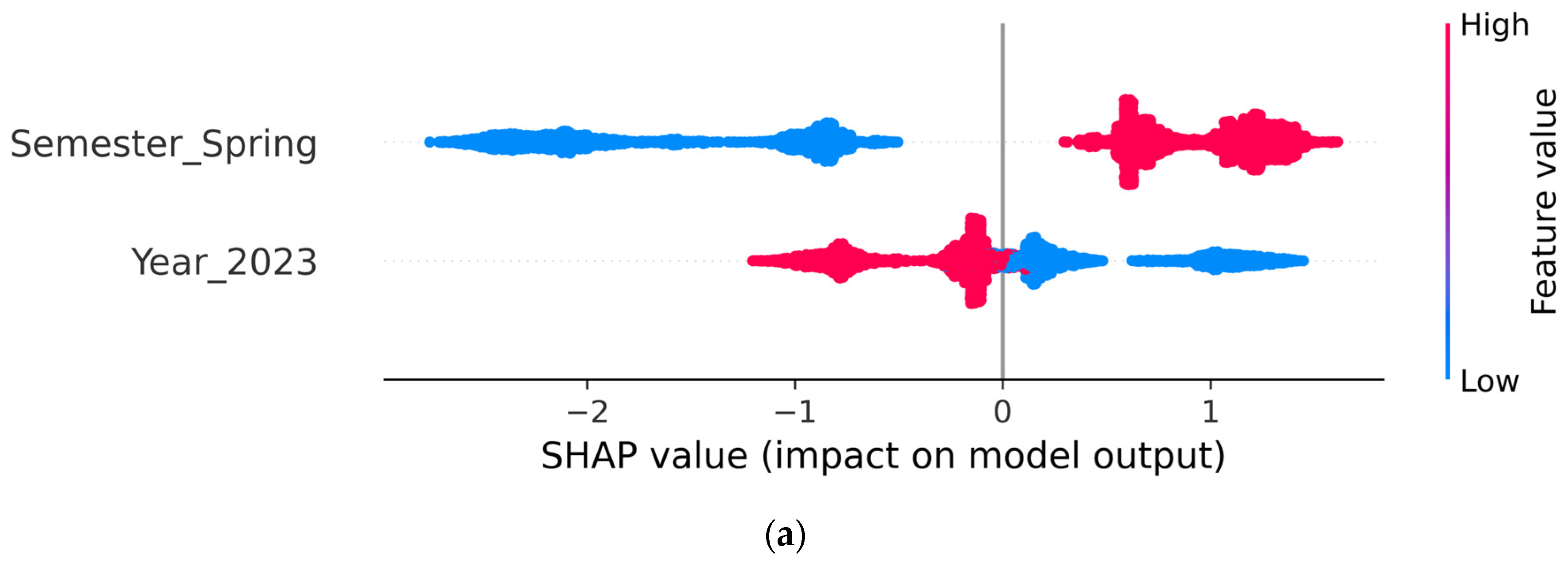
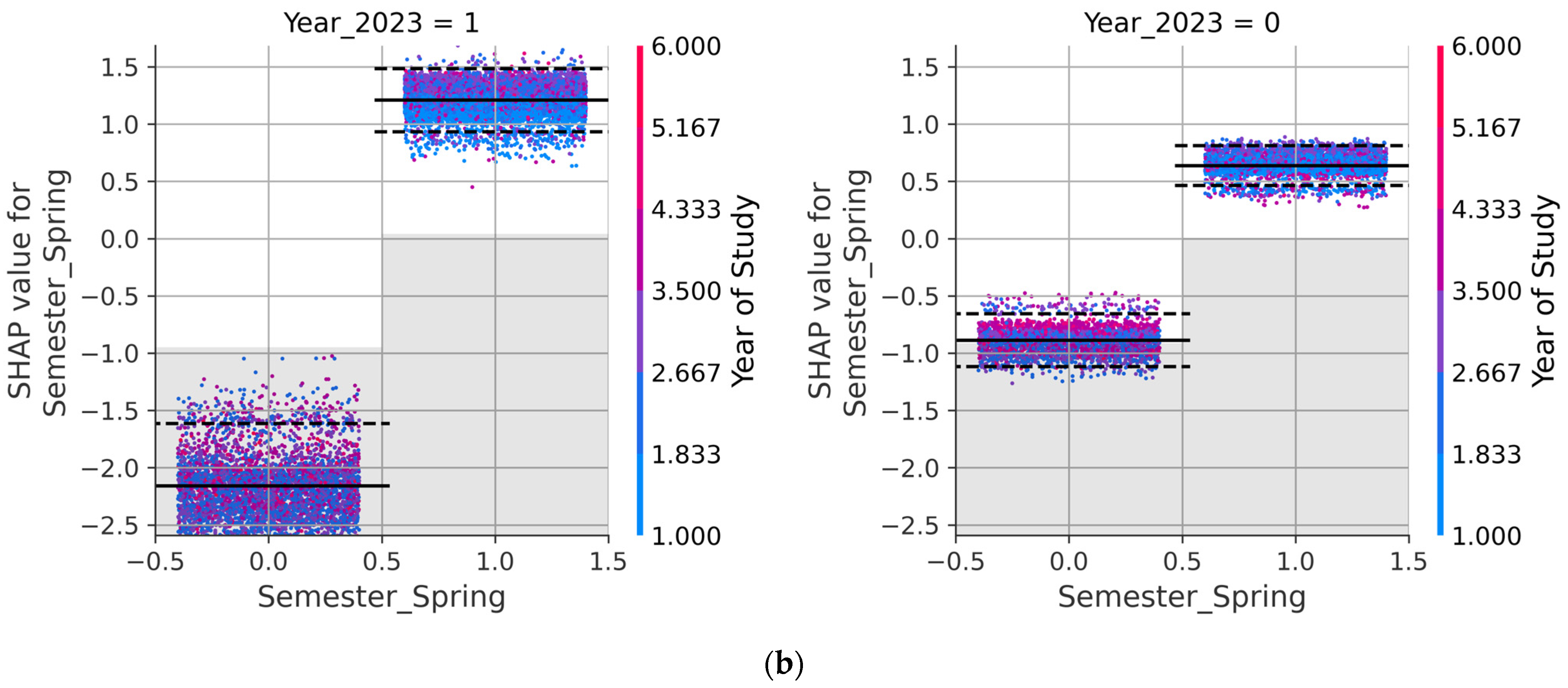
The variables Semester_Spring and Year_2023 rank among the top three most significant features across all studied models according to the SHAP feature importance metric. Figure 3a reveals that retaking exams from the previous Fall semester during the subsequent Spring semester increases the likelihood of failing retakes. Conversely, retaking exams in the Fall semester markedly reduces this probability.

Regarding Year_2023, the CatBoost model indicates higher retake success rates in 2023 compared to 2022.

Figure 3b shows that whether the academic year was 2023 or not strongly influenced retake outcome predictions:

• Retaking a debt from the Spring semester of 2022 in the Fall semester of 2023 reduced the probability of failure less than it would have in another academic year.
• Retaking a debt from the Fall semester of 2023 in the Spring semester of 2023 increased the probability of failure less than it would have in another academic year.

The XGBoost, LightGBM, and Random Forest models exhibit a similar pattern regarding the contribution of the Semester_Spring and Year_2023 features: retaking exams from the Fall semester increases the failure probability by 7–40%, whereas retaking exams from the Spring semester markedly decreases this probability (by 7% to 65%).

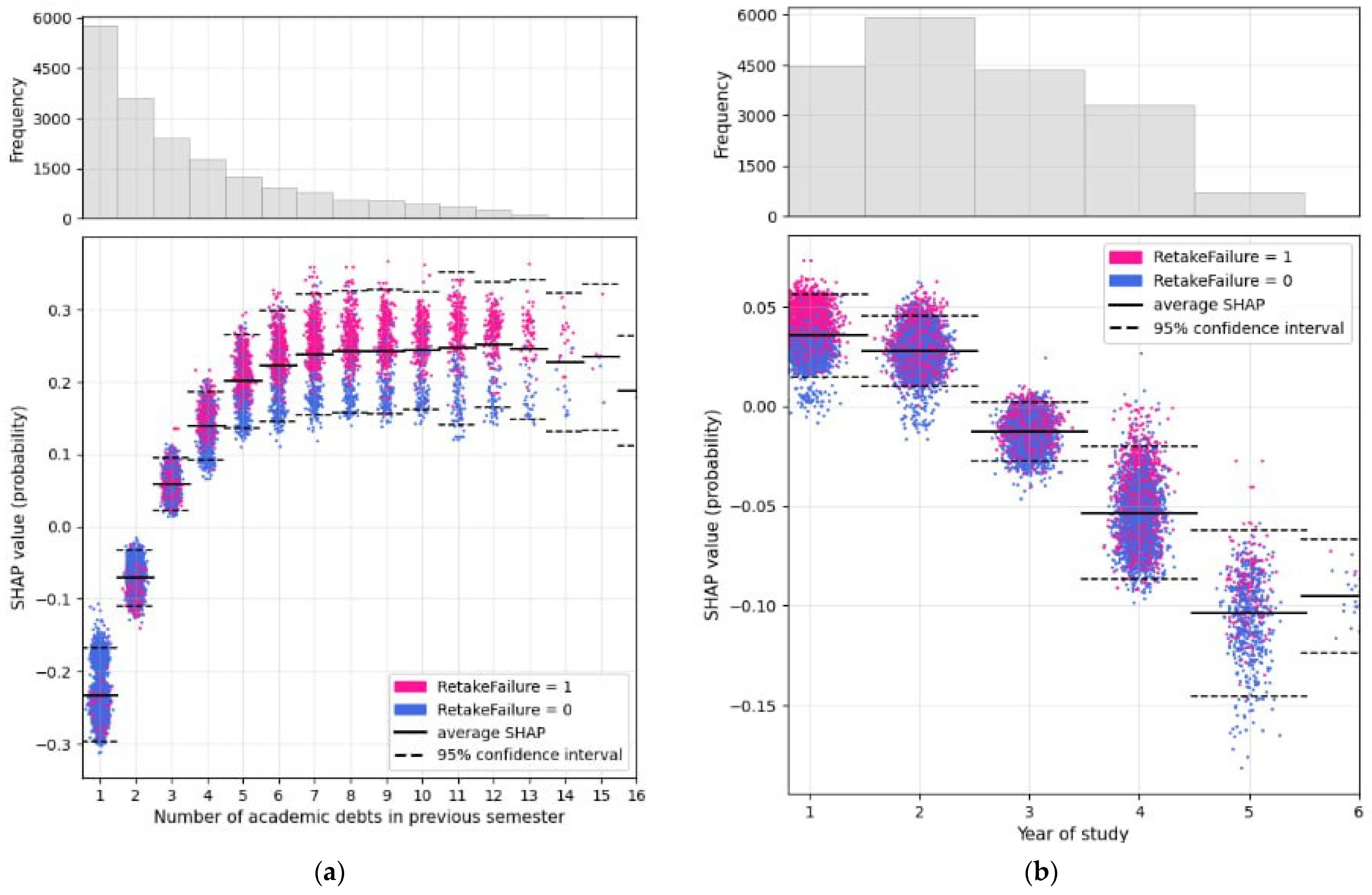
Figure 4 presents the distributions of SHAP values for the discrete variables—Number of academic debts in the previous semester and Year of Study.

Figure 4a reveals the following:

• The presence of one debt noticeably reduces the SHAP value (on average, the probability of failing the retake decreases by 24%).
• The presence of two debts also lowers the SHAP value (on average, the probability of failing decreases by 7%).
• The presence of three debts slightly increases the SHAP value (the probability of failing the retake increases by an average of 6.5%).
• For more than three debts, the 95% confidence intervals for the mean SHAP values overlap, and the average increase in SHAP ranges from 14% to 25% in terms of probability.

The other models exhibit a similar pattern regarding the effect of the number of previous-session debts on the likelihood of retake failure, with the exception of the Random Forest model, where the confidence interval for the mean SHAP values slightly extends into positive values.

As shown in Figure 4b

• Being a first- or a second-year student increases the probability of failing a retake for the CatBoost model, with an average increase of 3% and 2.5%, respectively.
• Being in the third year or higher consistently decreases the likelihood of failing retakes.

The other models exhibit a nearly identical pattern regarding the impact of second-year enrollment or above on the likelihood of retake failure. However, for the XGBoost and LightGBM models, being a first-year student is associated with an average increase in this probability of 6.75% and 6.5%, respectively.

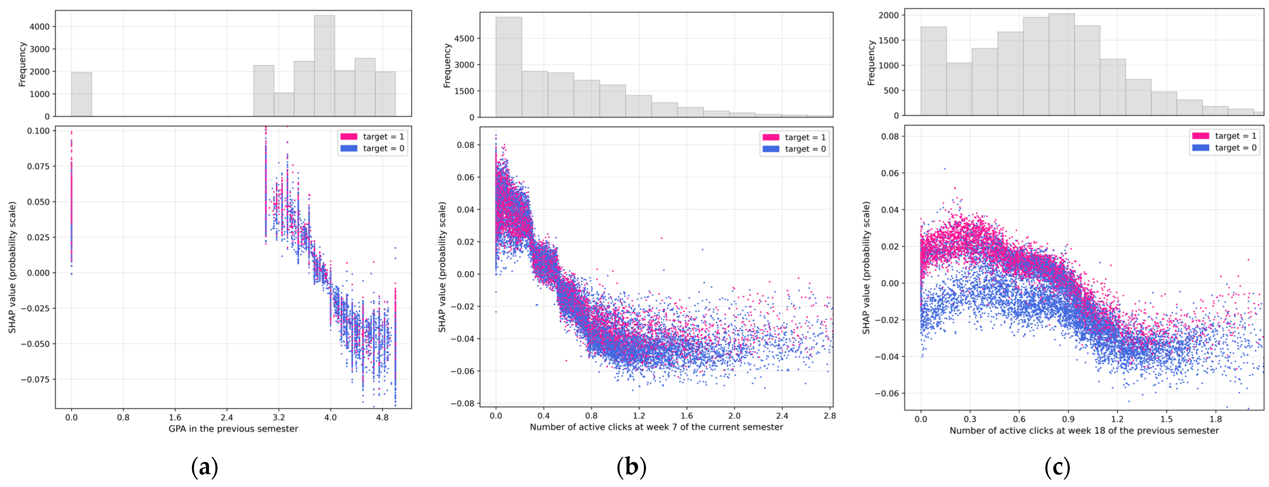
Figure 5 presents the SHAP distributions for three continuous predictors used in the forecasting models. Figure 5a displays the SHAP values for the variable GPA in the previous semester. It can be observed that a considerable number of students (1949 out of 18192) have a GPA of 0. This corresponds to situations where a student failed to pass any exams during the examination session. For the CatBoost model, a zero value for this variable consistently increases the probability of failing retakes (by 0–10%). GPA values ranging from 3 to 3.5 are associated with an increased probability of failing retakes, whereas a GPA of 4 or higher decreases this probability. This pattern holds for the other three models as well.

Figure 5b demonstrates the influence of the variable Number of active clicks at week 7 of the current semester on the model’s predictions. The value of this variable for a given student is calculated as follows: the number of active clicks they made is divided by the average number of active clicks in their study group (AVG_7_current). Thus, a value of this variable greater than one indicates that the student made more active clicks than the group average, while a value less than one indicates fewer clicks than the average.

As seen from the figure, for the CatBoost model, the SHAP values for Number of active clicks at week 7 decrease as the variable increases. Specifically, making fewer than 0.3·AVG_7_current clicks increases the probability of failing retakes (by an amount ranging from 0 to 8%), whereas making 0.5·AVG_7_current clicks decreases this probability (by 0 to 7%).

Regarding the other models, Random Forest demonstrates a similar pattern in how the Number of Active Clicks variable influences predictions, except that the reduction in the probability of failing retakes occurs after 0.7·AVG_7_current. In contrast, for the LightGBM and XGBoost models, no clear association was observed between specific values of Number of Active Clicks and an increased or decreased likelihood of failing retakes.

Figure 5c indicates that values of Number of active clicks at week 18 of the previous semester greater than 1.1·AVG_18_previous decrease the risk of failing retakes. Below this threshold, no clear pattern emerges. AVG_18_previous represents the average number of active clicks in a study group at week 18 of the previous semester.

Both the XGBoost and LightGBM models associate the Number of active clicks at week 18 greater than 0.85·AVG_18_previous with a 3–13% decrease in probability of failing retakes, whereas Random Forest reduces this probability by 0.1–0.8% for values of Number of active clicks at week 18 exceeding 0.9·AVG_18_previous.

Among predictors not in the top five by SHAP feature importance, consistent influences on model predictions are observed for two variables: Average grade for all e-courses at week 18 of the previous semester and School_16.

The variable Average grade for all e-courses at week 18 for a given student is calculated as the student’s average grade for e-courses in which they were enrolled at week 18 of the previous semester, divided by the average of this characteristic within their study group (AVG_grade_18_previous). According to all four models, the probability of a student failing retakes decreases by 0–9% when their Average grade for all e-courses at week 18 is greater than or equal to 1.05·AVG_grade_18_previous.

The variable School_16 equals 1 if the student is enrolled at the university’s branch—the Lesosibirsk Polytechnic School—and 0 otherwise. According to all models, the probability of a student failing retakes is substantially reduced if they are studying at the Lesosibirsk Polytechnic School (by an amount ranging from 20% to 80%). Moreover, we found that out of the 152 students from this school included in our dataset, only three failed to clear their academic debts during retakes.

3.2. Identifying Student Risk Groups for Retakes Based on SHAP Analysis Findings

Having identified the most influential predictors and characterized their impact on model forecasts, we applied the SHAP analysis results to determine which combinations of these predictor values can reliably stratify students into distinct risk categories before retakes. This will be beneficial for providing targeted pedagogical support to students.

To ensure generalizability, we excluded predictors reflecting institution-specific characteristics (e.g., School_16) or temporary cohort effects (e.g., Year_2023). Instead, we concentrate on stable, generalizable student-level metrics and curriculum-structural features that can be reliably and consistently monitored across future academic years.

For each year of study and both academic semesters, we will identify the following risk groups among the students:

• Red group—very high risk, characterized by an unsuccessful retake rate of 90% or higher;
• Yellow group—high risk, with an unsuccessful retake rate between 75% and 90%;
• Green group—low risk, with an unsuccessful retake rate of no more than 5%.

We will characterize these groups using models’ features that demonstrated consistent influence on models’ predictions in Section 3.1.

The profiles of the selected groups for Spring semesters are presented in

Table 6. Profiles of Student Risk Groups for Retakes in Spring Semesters.

Year of Study, Number of Students/Percent Failing Retakes	Feature	Red	Yellow	Green
First, 4460/53%	Number of academic debts in previous semester	≥2	≥2	1
	GPA in the Previous Semester	≤4	≤4	>4.75
	Average grade for all e-courses at week 18 of the previous semester	any	any	≥1
	Number of active clicks at week 18 of the previous semester	<0.1	<1	≥0.8
	Number of active clicks at week 7	<0.1	any	any
Number of Students/Percent Failing Retakes		333/90%	1926/76%	64/5%
Second, 3024/56%	Number of academic debts in previous semester	>3	≥2	1
	GPA in the Previous Semester	<3.6	<3.7	≥4.3
	Average grade for all e-courses at week 18 of the previous semester	<0.9	any	>0.95
	Number of active clicks at week 18 of the previous semester	<0.75	any	>0.95
	Number of active clicks at week 7	<0.3 *	any	any
Number of Students/Percent Failing Retakes		219/90%	1168/79%	150/5%
Third, 2246/57%	Number of academic debts in previous semester	>3	≥2	1
	GPA in the Previous Semester	<3.2	<3.6	≥4.3
	Average grade for all e-courses at week 18 of the previous semester	<0.75	any	>1
	Number of active clicks at week 18 of the previous semester	<0.9	any	>1.1
	Number of active clicks at week 7	<0.2 *	any	any
Number of Students/Percent Failing Retakes		97/91%	758/78%	63/5%
Fourth, 1534/43%	Number of academic debts in previous semester	>3	≥2	1
	GPA in the Previous Semester	<3.2	<3.5	≥4.4
	Average grade for all e-courses at week 18 of the previous semester	<0.75	any	>1
	Number of active clicks at week 18 of the previous semester	<0.9	<0.9	>0.9
	Number of active clicks at week 7	<0.2 *	any	any
Number of Students/Percent Failing Retakes		52/92%	250/78%	66/5%
Fifth, Sixth 251/35%	Number of academic debts in previous semester	>3	≥3	1
	GPA in the Previous Semester	<3.2	<3.4	≥4.4
	Average grade for all e-courses at week 18 of the previous semester	any	<0.3	any
	Number of active clicks at week 18 of the previous semester	any	any	any
	Number of active clicks at week 7	<0.3 *	any	any
Number of Students/Percent Failing Retakes		10/90%	17/76%	19/5%

* and ≠0.

.

In summary, Table 6 demonstrates that monitoring a small set of indicators—two from the digital educational profile and three from the digital footprint—allows for the effective stratification of students into distinct risk categories for retake failure in Spring semesters. The thresholds for inclusion in high-risk groups are lower for students in earlier years. While the presence of two or more academic debts from the previous semester serves as a primary risk signal, first-year students were classified into the Yellow group if their prior semester GPA was ≤4 and their active clicks by the end of that semester were below the group average. In contrast, more advanced students required a more pronounced academic decline to be considered at-risk: for example, a third-year student with two or more debts was assigned to the Yellow group only if their prior semester GPA fell below 3.6.

Notably, LMS engagement metrics proved valuable for identifying both high- and low-risk student groups. Following the Fall semester examination period, data on active clicks and e-course scores—combined with GPA and prior academic debts—were sufficient to assign students to the Yellow and Green risk categories. Moreover, extremely low engagement in the electronic environment by the seventh week of the subsequent semester was associated with a sharply increased risk of retake failure, reclassifying students from the Yellow to the Red group and signaling the need for heightened attention and targeted support measures.

Retakes occurring in the Fall semester were associated with a substantially lower probability of failure, as previously shown in Figure 3a. The empirical failure rates for Fall-semester retakes were 17% for 2908 second-year students, 19% for 2112 third-year students, 28% for 1768 fourth-year students, and 17% for 499 fifth- and sixth-year students. Consequently, it was not feasible to establish Red and Yellow risk groups for the Fall semesters. The Green groups, however, were notably large for each cohort and consisted of students who satisfied the following criteria:

• Second-year students (1028 students, 2% of them failed retakes): Number of academic debts in previous semester ≤ 3, GPA in the Previous Semester > 3, Average grade for all e-courses at week 18 of the previous semester > 0, Number of active clicks at week 18 of the previous semester > 0.
• Third-year student (776 students, 2% of them failed retakes): Number of academic debts in previous semester ≤ 5, GPA in the Previous Semester ≥ 3, Average grade for all e-courses at week 18 of the previous semester > 0, Number of active clicks at week 18 of the previous semester > 0.
• Fourth-year students (600 students, 4% of them failed retakes): Average grade for all e-courses at week 18 of the previous semester > 0.
• Fifth- and sixth-year students (600 students, 0% of them failed retakes): Average grade for all e-courses at week 18 of the previous semester > 0.

In summary, it was found that fourth-year students and above who exhibited any activity in the electronic environment during the prior Spring semester were almost certain to succeed in their retakes. For junior students, however, the criteria for Green group classification were more restrictive, incorporating additional thresholds for number of academic debts and GPA—with requirements being less stringent for third-year students and more stringent for second-year students.

Using first-year students as an example, we will consider one possible way to apply the identified risk group profiles for the pedagogical support of students in order to reduce the percentage of unsuccessful retakes. Table 4 shows that the number of first-year students with outstanding academic debts from the previous (Fall) semester is quite large—4460 students over the 2022–2024 academic years. Therefore, it would, first, be advisable to identify students with a high risk of failure on retakes immediately after the examination period, based on their exam results, digital profile, and digital footprint from the previous semester, in order to begin intensified support work with them right away. Second, to reduce the workload of instructors and tutors, it would be useful to identify students with a low risk level, who are likely to successfully manage their retakes without pedagogical assistance.

Pedagogical support will be provided to students in the Yellow group, which consists of 1926 students, while the 64 students in the Green group can be left without intervention. For the remaining students—those classified as neither Green nor Red—we will simply monitor their learning progress from the beginning of the next semester. By the seventh week of the following semester (approximately one to two weeks before the start of the retake period), data on their current educational behavior become available. The variable Number of active clicks at week 7 essentially serves as a marker of the extent to which a student is engaged in the ongoing learning process. Knowledge of its values allows us to identify students in the Red group—in our case, it consists of 333 students. For these students the intensity of pedagogical support needs to be increased, potentially including new forms of assistance that were not provided to students in the Yellow group.

3.3. SHAP Analysis for Models Predicting Dropouts

To effectively monitor students at the subsequent stage—between an unsuccessful initial retake and potential dropout following a failed commission retake—it is essential to understand which aspects of the academic trajectory the Level-2 Models rely upon.

A comparative analysis of four machine learning algorithms—CatBoost, LightGBM, XGBoost, and Random Forest—revealed comparable prediction quality on the test sample (F1 ≈ 0.85); however, analysis of feature ranking revealed fundamental differences in their focus, with some models relying on behavioral metrics from the digital footprint and others on static characteristics of the students’ academic profile. The feature space of the models comprised three variable categories:

• Behavioral digital footprint metrics: Inactivity periods (Downtime_week_4, Downtime_sem1_week_10, Downtime_sem1_week_18), active clicks (Number of active clicks at week 4, Number of active clicks at sem1 week 10, Number of active clicks at sem1 week 18), effective clicks, and LMS performance measured at the specific weeks of the semester.
• Academic profile characteristics: Year of Study, Semester, academic year, institute affiliation.
• Academic indicators: Number of academic debts after first session, Number of academic debts after second retake, Funding type.

Analysis of the top-10 features by importance in the CatBoost model revealed the dominance of behavioral digital footprint metrics. The top three positions are occupied exclusively by LMS activity features from the fourth week of the current semester: Downtime_week_4, Number of active clicks at week 4, and Number of effective clicks at week 4. The academic indicator Number of academic debts after first session occupies only the fourth position, while profile characteristics appear in the top-10 with importance values several times lower than the leading behavioral features. CatBoost interprets dropout risk primarily through the lens of the student’s current interaction with the digital educational environment.

In contrast to CatBoost, LightGBM demonstrates a shift toward static characteristics of the academic profile. The feature Downtime_week_4 retains the leading position; however, the second and third positions are occupied by academic indicators and profile characteristics: Number of academic debts after first session and Semester_Fall. Year of Study appears in the top-5, and Number of academic debts after second retake enters the top-10, indicating increased model attention to the students’ history of academic difficulties.

The XGBoost model demonstrates the most balanced feature importance structure, where behavioral digital footprint metrics and academic profile characteristics appear in the top 10 with comparable values. The model forms predictions based on an integral representation of the student, combining current LMS behavior, academic history, contextual factors, and institutional affiliation.

By comparison, Random Forest relies almost exclusively on academic profile characteristics and academic indicators.

The most significant feature group by SHAP values across all models comprises current-semester behavioral features in the electronic environment. These indicators were specifically selected for model training because commission retakes typically occur within the first month of the semester. They reflect a hierarchical structure of LMS interaction: baseline engagement and authorization (Downtime, Number of active clicks), quality of interaction through result-oriented actions (Number of effective clicks), and academic performance in a course (Score).

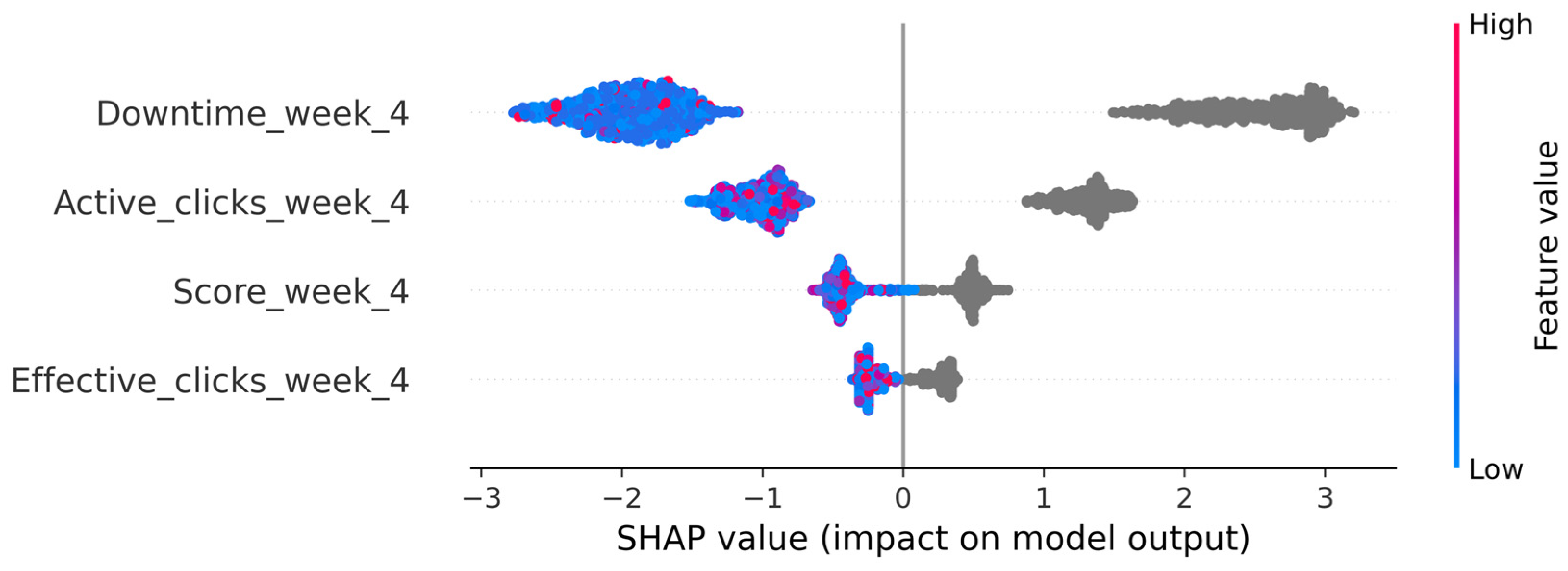
Figure 6 presents SHAP summary plots for these behavioral features. The visualizations reveal that Downtime_week_4 is the most influential feature across all models. Importantly, it functions as a threshold indicator: any value indicating activity reduces the probability of dropout. A similar protective pattern is observed for Number of active clicks at week 4, Number of effective clicks at week 4 and Score_week_4.

The gray points in Figure 6 represent students who had no recorded interaction with the LMS by week 4 of the semester. This absence of a digital footprint constitutes a distinct behavioral pattern indicating complete disengagement from the electronic learning environment during the critical post-retake period.

Analysis of digital footprint trajectories at weeks 4 and 10 reveals three distinct student groups (

Table 7. Distribution of students by digital footprint patterns at weeks 4 and 10 of the semester (n = 1916).

Student Group	Count	Share of Group with Missing Data at Week 4	Dropout Rate
Persistent absence (missing data at weeks 4 and 10)	573	82.7%	55.5%
Late emergence (missing data at week 4, data present at week 10)	120	17.3%	0%
Stable presence (data present at weeks 4 and 10)	1223	0%	0%

).

The high correlation between the absence of digital footprint at week 4 and week 10 (r = 0.868, p < 0.001), combined with the dominance of the persistent absence group (82.7% of cases), confirms that this represents a stable behavioral pattern of prolonged disengagement. Furthermore, the strong internal correlation among the Week 4 metrics (e.g., r = 0.994, p < 0.001 between Downtime_week_4 and Number of active clicks at week 4) reflects the logical structure of LMS interaction: absence of a system login precludes all derived activity metrics.

The absence of a digital footprint emerges as a critical behavioral predictor of dropout. In the studied cohort, all 318 dropout cases occurred exclusively among students without recorded LMS interaction by week 4 (n = 693). Conversely, students with any documented activity in the system (n = 1223) exhibited a 0.0% dropout rate, regardless of their academic history. This finding establishes the presence/absence of a digital footprint at week 4 as a robust, pedagogically meaningful indicator. Consequently, the monitoring system should treat LMS non-interaction as a primary behavioral signal requiring immediate intervention.

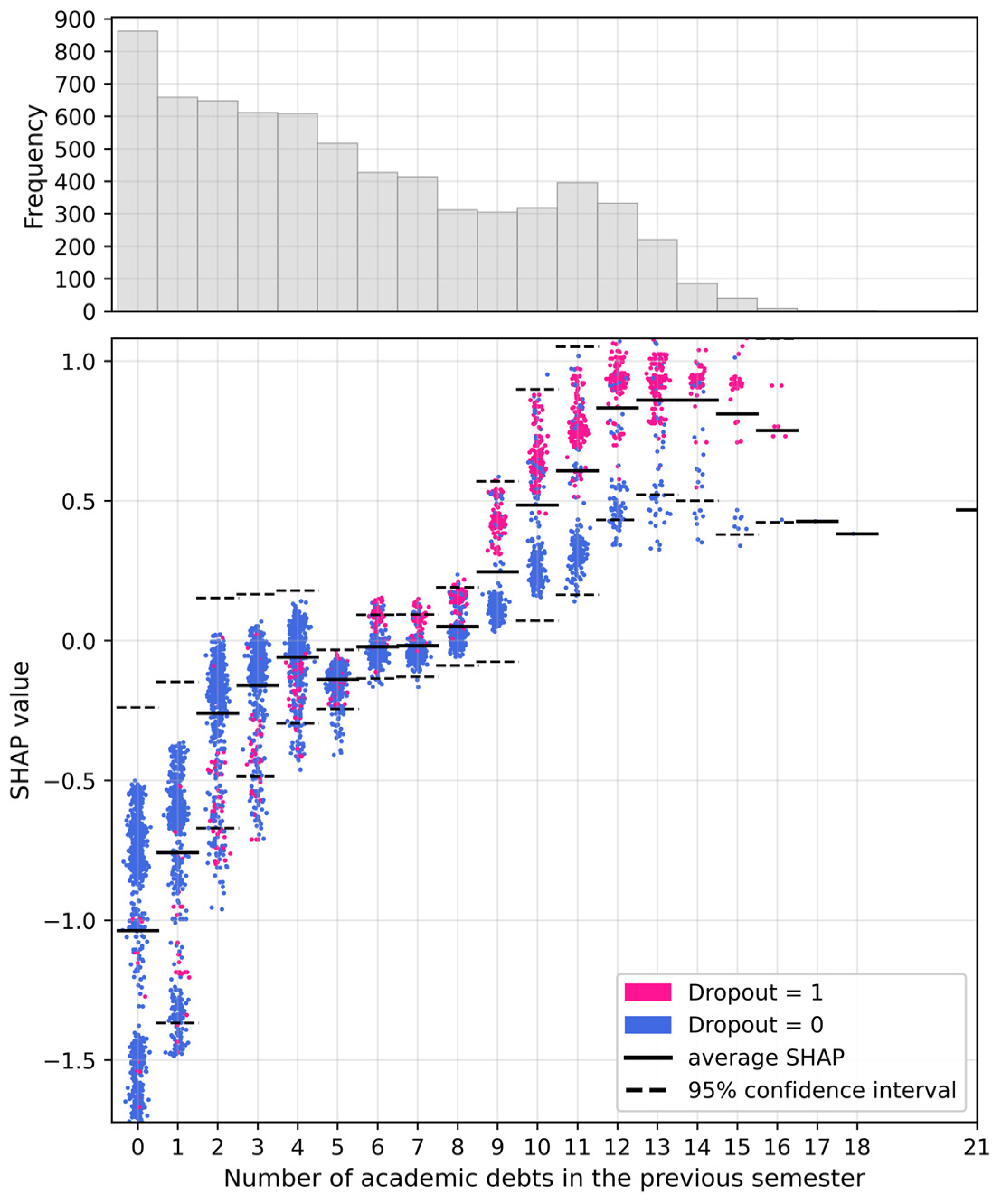
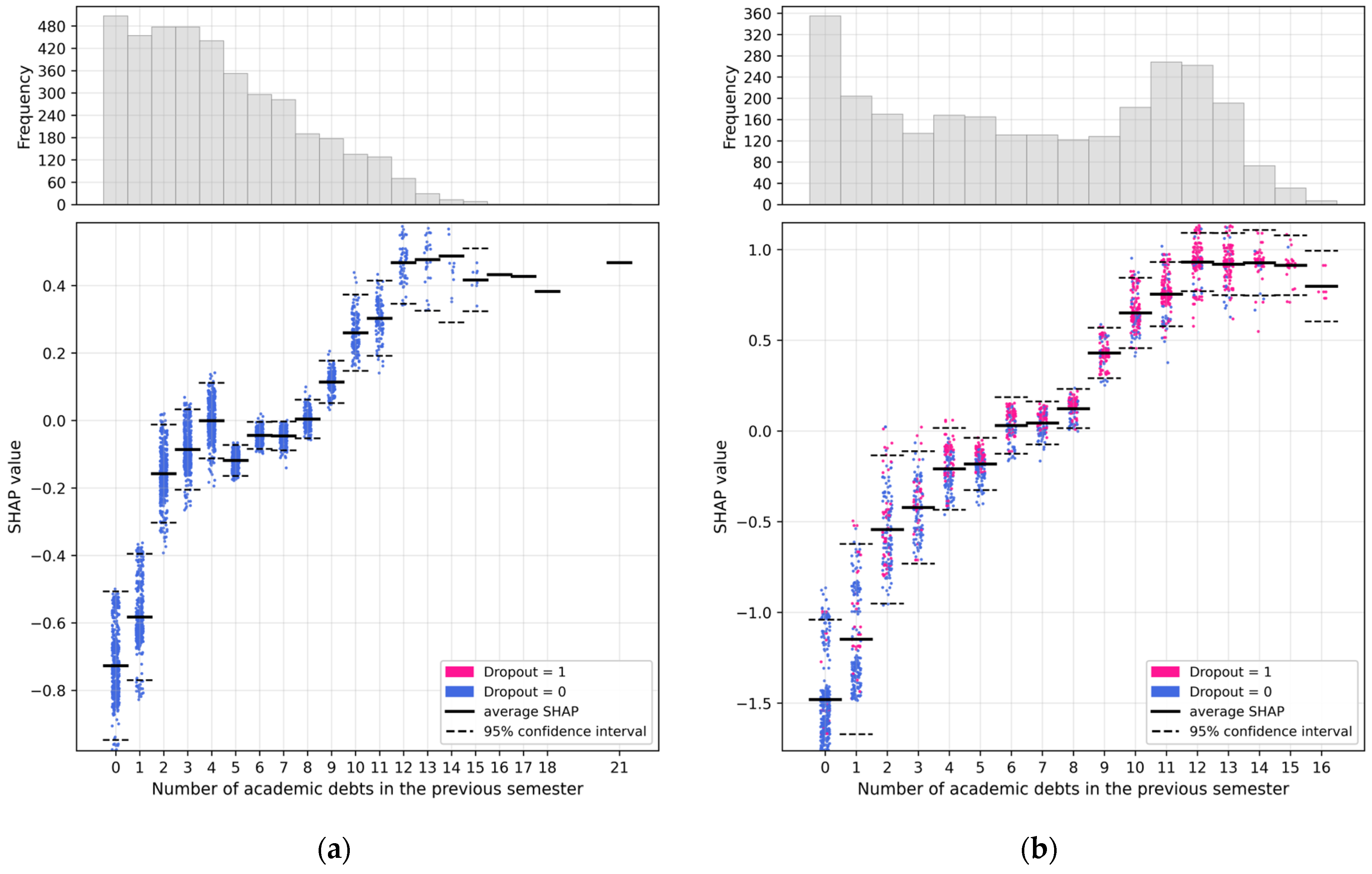
The feature Number of academic debts in previous semester occupies high positions in the global importance ranking across all models. Analysis of local SHAP values revealed a non-linear dependence of risk on the number of debts, with a critical threshold at 8–9 debts (Figure 7).

Across all models, a sharp transition is observed from negative or near-zero SHAP values at 0–8 debts to pronounced positive values at ≥9 debts. For the CatBoost model, the mean SHAP value is −0.485 ± 0.482 at 0–2 debts, −0.319 ± 0.139 at 3–5 debts, −0.081 ± 0.386 at 6–8 debts, followed by a sharp rise to 1.237 ± 0.397 at ≥9 debts. The LightGBM model demonstrates a smoother transition: from −0.596 ± 0.474 at 0–2 debts to 0.695 ± 0.256 at ≥9 debts, with monotonic growth in intermediate ranges (Figure 7). For the XGBoost model, the mean SHAP value increases from 0.158 ± 0.175 in the 6–8 academic debts category to 0.935 ± 0.229 for students with ≥9 debts, indicating a stronger positive contribution to dropout risk at higher debt levels. The Random Forest model exhibits a gradual monotonic increase from −0.105 ± 0.084 in the 0–2 debts category to 0.125 ± 0.060 for students with ≥9 debts, with consistently smaller SHAP value magnitudes indicating more conservative feature contributions to dropout risk prediction”.

Analysis of the interaction Number of academic debts in previous semester × Presence of digital footprint in Figure 8 showed that the presence of minimal interaction with the electronic learning environment at week 4 of the semester is strongly associated with a near-zero observed dropout rate, regardless of the accumulated number of debts. Among students with a digital footprint, the dropout rate is 0.0% across all debt load ranges, including the critical threshold ≥ 9 debts. In contrast, among students without a digital footprint, dropout risk monotonically increases with debt load: from 13.0% (0–2 debts) to 33.6% (3–5 debts), 46.9% (6–8 debts), and reaches 77.0% at ≥9 debts.

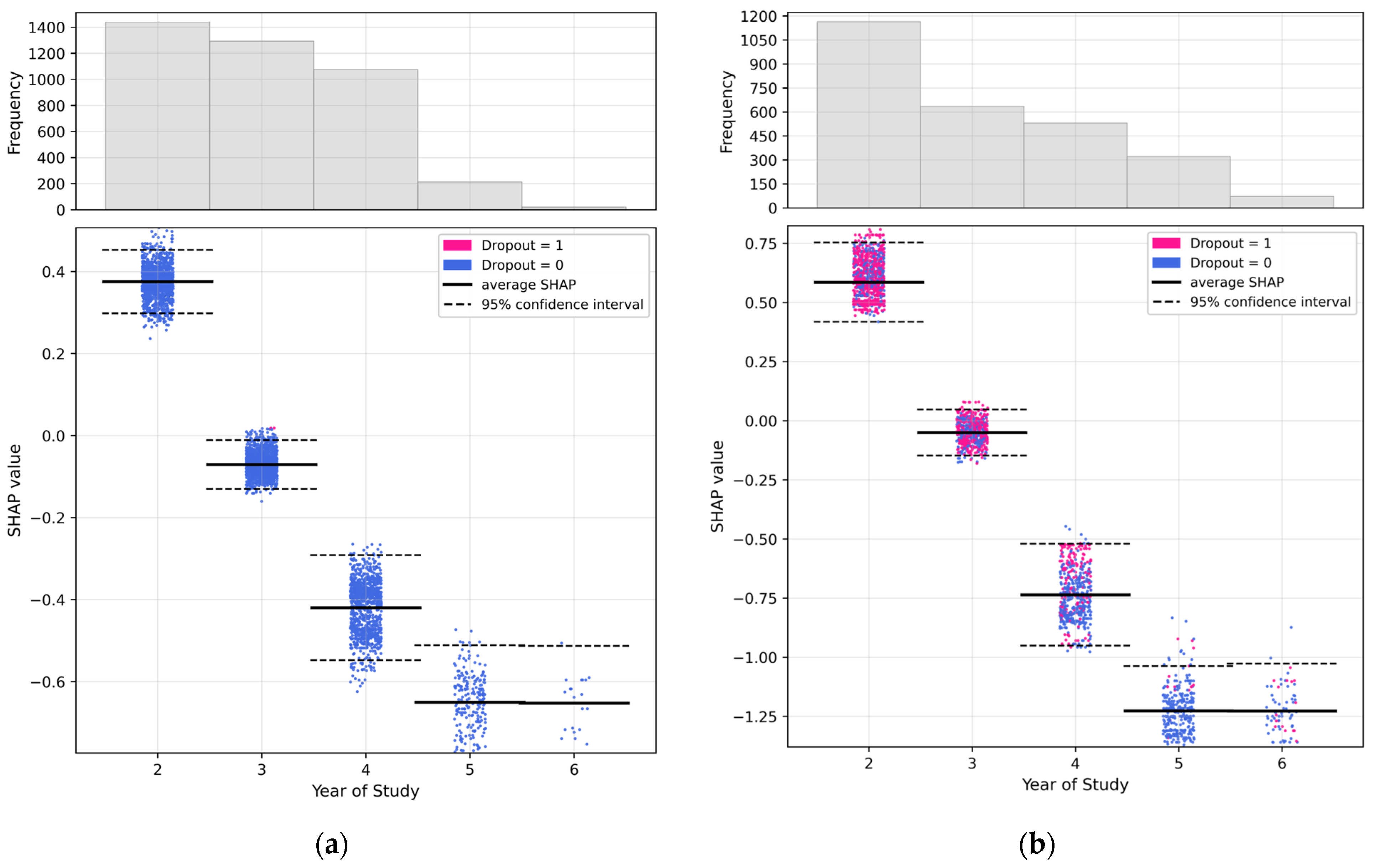
Year of Study exhibits a pronounced monotonic relationship: dropout risk decreases progressively from the second to the fifth year. For the LightGBM model, the mean SHAP value is 0.469 ± 0.123 in the second year, −0.064 ± 0.039 in the third year, −0.524 ± 0.17 in the fourth year, and −0.997 ± 0.296 in the fifth year. The dropout rate decreases from 33.4% in the second year to 19% in the third year, 10.5% in the fourth year, and 2.6% in the fifth year. In the second year, students first face the threat of dropout due to academic debts after completing the adaptive first year, creating a peak of vulnerability in the academic trajectory.

Among students without a digital footprint at week 4 of the second year, the mean SHAP value reaches 0.586 with a dropout rate of 74.7%, whereas among students with a digital footprint, the mean SHAP value decreases to 0.375 with a dropout rate of 0.0%. A similar pattern is observed in the fourth year: the absence of a footprint is associated with a dropout risk of 31.8%, whereas the presence of a footprint is associated with zero risk. The presence of student interaction with the LMS is consistently associated with substantially lower observed dropout rates across all years of study (Figure 9).

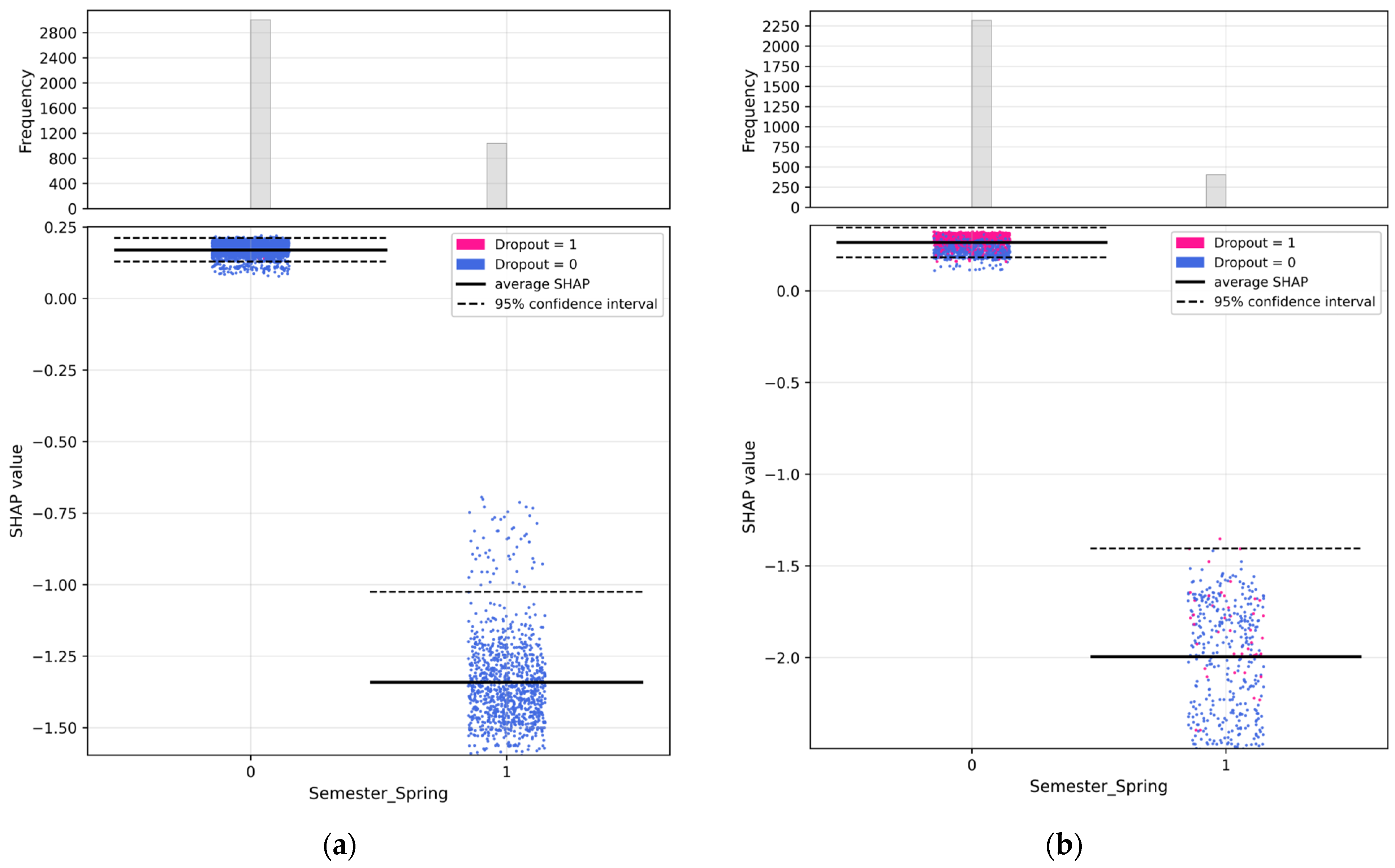
The feature Semester shows that the Fall semester is associated with an increased dropout risk (26.1%), whereas the Spring semester is associated with the minimal risk (3.1%). For the LightGBM model, the mean SHAP value is 0.211 ± 0.056 for the Fall semester and −1.525 ± 0.361 for the Spring semester.

Among students in the Fall semester without a digital footprint, the dropout rate reaches 59.9% with the mean SHAP value of 0.263, whereas among students with a digital footprint, the dropout rate is 0.1% with the mean SHAP value of 0.170 (Figure 10).

3.4. Identifying Student Risk Groups for Dropouts Based on SHAP Analysis Findings

Based on the conducted analysis of global feature importance and local explanations using the SHAP method, key factors determining the risk of student dropout following an unsuccessful retake were identified. For the practical application of modeling results within the academic failure monitoring system, we define three student risk categories based on the empirical dropout rate within subgroups formed by combinations of key feature values. In contrast to the task of predicting unsuccessful retakes, more conservative boundaries were established for the dropout prediction task: a Red group with a risk greater than 75%, a Yellow group with a risk from 50% to 75%, and a Green group with a risk up to 5%. This reflects the critical and irreversible nature of dropout; even moderate risk in the Yellow group requires active pedagogical intervention.

The profiles of the identified groups based on the most important features are presented in

Table 8. Profiles of Student Risk Groups for Dropout in Fall Semesters.

Year of Study, Number of Students/Percent of Dropout	Feature	Red	Yellow	Green
Second, 554/33%	Downtime at week 4 of the current semester	NaN	NaN	any
	Number of academic debts in previous semester	≥9	≤5	≤2
	Average grade for all e-courses at week 4	-	-	>1
	Number of active clicks at week 4 of the current semester	-	-	>0.8
Number of Students/Percent of Dropout		166/87%	51/65%	314/0%
Third, 412/19%	Downtime at week 4 of the current semester	NaN	NaN	any
	Number of academic debts in previous semester	≥9	≤5	≤2
	Average grade for all e-courses at week 4	-	-	>0.6
	Number of active clicks at week 4 of the current semester	-	-	>0.6
Number of Students/Percent of Dropout		54/76%	74/60%	286/0%
Fourth, 341/9%	Downtime at week 4 of the current semester	-	NaN	any
	Number of academic debts in previous semester	-	≥9	≤2
	Average grade for all e-courses at week 4	-	-	>0.7
	Number of active clicks at week 4 of the current semester	-	-	>0.6
Number of Students/Percent of Dropout		-	28/54%	241/0%
Fifth, Sixth, 140/4%	Downtime at week 4 of the current semester	NaN	-	NaN or any
	Number of academic debts in previous semester	≥6	-	≤2
	Average grade for all e-courses at week 4	-	-	>0.6
	Number of active clicks at week 4 of the current semester	-	-	>0.5
Number of Students/Percent of Dropout		6/83%	-	134/0%

. The table includes only those features that demonstrated a stable influence on the predictions of all four models and possessed an interpretable pedagogical meaning.

Table 8 demonstrates that monitoring a small set of indicators allows for effective stratification of students into separate dropout risk categories in the Fall semester. Having nine or more academic debts after the previous retake serves as the primary risk signal for second- and third-year students; for senior students, the critical threshold decreases to six debts.

Engagement metrics in the electronic educational environment proved valuable for identifying both high- and low-risk groups. The presence of minimal interaction with the learning environment, combined with a low debt load (≤2 debts) and moderate activity (>0.5–0.8 click share relative to the average student in the group), corresponds to a Green risk profile with an observed dropout rate of 0.0% across all years of study. Conversely, a complete absence of a digital footprint combined with a debt load above the critical threshold is associated with a dropout risk of 76–87%, requiring intensive pedagogical intervention.

The Fall semester is associated with a higher probability of dropout compared to the Spring semester. Empirical dropout rates constitute 33% for 554 second-year students, 19% for 412 third-year students, 9% for 341 fourth-year students, and 4% for 140 fifth- and sixth-year students. For the fourth year and above, it was not possible to identify a Red risk group due to the absence of subgroups with a risk ≥ 75%.

Senior students having any activity in the electronic environment in the fourth week of the semester are practically guaranteed to avoid dropout. For junior courses, the criteria for belonging to the Green group are stricter and include additional thresholds for the number of debts and the level of activity in the electronic environment.

The Spring semester demonstrates a different dropout risk pattern compared to the Fall semester. Empirical dropout rates in the Spring period are extremely low: 6% for 163 second-year students, 4% for 115 third-year students, 1% for 140 fourth-year students, and 0% for 26 fifth-year students.

Due to the low baseline risk level in the Spring semester, it is not possible to identify Red and Yellow risk groups: all students with a low debt load of less than 2 debts and minimal academic activity form a single Green group with zero dropout risk.

Identifying these risk groups allows for the optimization of resource allocation for curators, tutors, and academic staff by concentrating active interventions on students with critical and high dropout risk, while maintaining minimal monitoring for low-risk students. Analysis of student distribution across risk groups in the Fall semester shows that the Green group constitutes 64.4% of the entire sample, with almost zero dropout risk. In contrast, the empirical dropout rate within the Red group is 84.5%, while the Yellow group shows a dropout rate of 60.5%. This uneven risk distribution allows for reducing the workload on curators by excluding active monitoring of the Green group, which matters given limited university resources. At the same time, focusing attention on students in the Red and Yellow groups allows covering 92% of all potential dropout cases, ensuring maximum efficiency of pedagogical support with minimal resource expenditure.

Using the example of second-year students in the Fall semester (554 students), we suggest a possible way to apply the identified risk group profiles for pedagogical support aimed at reducing the dropout rate. It is advisable to identify students with a critical dropout risk immediately after the completion of the Spring semester session, based on their debt load and the digital profile from the previous semester, to begin intensive work with them as early as possible. To reduce the workload on curators and tutors, low-risk students should be identified. These students can successfully pass the commission retake without active intervention, owing to their digital footprint, low debt load, and moderate activity in the electronic environment. Students in the Yellow group require preventive support and weekly monitoring of the digital footprint.

For the Red group, early outreach aimed at understanding barriers to LMS engagement may serve as a strategic initial step. However, such engagement should be interpreted as a prognostic trigger for allocating intensive support, rather than a direct causal lever for retention.

4. Discussion

4.1. Scalability and Operational Efficiency of the SHAP-Based Approach for Monitoring At-Risk Students

The two-level monitoring system for at-risk students, based on predictive models and SHAP analysis as proposed in this article, can be scaled to varying degrees across diverse educational contexts.

Broadly, the proposed approach for identifying significant indicators of academic failure can be adopted by universities operating under diverse academic debt management policies.

The implementation framework can be structured as follows:

• Develop separate models for each stage of an underperforming student’s educational trajectory to predict academic failure, using the educational data available for collection and analysis at that particular university.
• Identify a pool of best-performing models for each stage.
• Conduct SHAP analysis on all predictors—or at least the most significant ones—within these predictive models. This analysis can be supplemented by an examination of the consistency in the patterns of dependence between these predictors and the models’ forecasts. If a particular pattern is observed in most of the predictive models, this suggests that the relationship between the corresponding predictors and the model forecasts is robust and consistent.
• Build the set of monitoring indicators for educational behavior and academic performance based on the predictors that demonstrated significant and consistent relationships with student failure in the previous step.
• Use these indicators to construct student risk profiles that correspond to varying degrees of risk for future academic failure, enabling the effective scaling of pedagogical response.

The findings of our study regarding the most significant indicators of disengagement and future academic failure may also be applied to educational institutions with similar learning conditions and grading policies.

In particular, most universities maintain databases of examination session results and educational profile indicators, from which important variable indicators such as previous semester debts and GPA can be obtained. Furthermore, e-learning is often conducted through Moodle or similar LMS platforms, which allow access to the same types of indicators used in our study—specifically, active clicks, effective clicks, downtime and the average score in e-courses during different weeks of instruction.

If such similarity in learning conditions and policies is indeed present, the significant predictors of student failure identified in our study can be recommended for incorporation into the development of academic failure predictive models, with the set of predictors being expanded to include university-specific features.

The undeniable advantage of using SHAP explanations is their interpretability. This method isolates the specific contributions of individual risk indicators to the overall prediction, resulting in a set of simple, interpretable metrics. Moreover, this approach helps reduce ongoing operational costs associated with the extensive collection and processing of data. Once an institution has conducted this analysis using complex predictive models with a large number of features, the ongoing operation of those models can be discontinued. Instead, universities can monitor only the key indicators of academic failure identified through SHAP analysis.

4.2. Applicability of SHAP Interpretations for Models with Varying Prediction Quality

The two-level monitoring system proposed in this study sequentially applies machine learning models at distinct stages of the student academic trajectory. A limitation of this research is the difference in predictive performance between Level-1 and Level-2 Models. The retake outcome prediction models demonstrate moderate quality on the test sample (accuracy ≈ 0.81–0.82, F1-score ≈ 0.75–0.76), whereas the dropout prediction models achieve high quality (accuracy ≈ 0.95–0.96, F1-score ≈ 0.84–0.89).

The difference in model quality is attributable to both data characteristics and differences in assessment procedures for retakes and commission retakes. The retake process following an unsuccessful examination session is less formalized compared to commission retakes. Assessment during initial retakes is more subjective, given that different instructors employ varying evaluation approaches, and the retake procedure differs by discipline and institute. In contrast, commission retakes preceding dropout are conducted in a strictly regulated format: the examination commission consists of three specialists, the evaluation procedure is standardized and documented in official records, and commission decisions are made collectively. This formalization minimizes the influence of subjectivity and random factors and creates more reliable conditions for prediction, which explains the higher quality of the Level-2 Models in the system.

It is important to note that the quality limitations of the retake outcome prediction models are not critical for the functioning of the monitoring system, as after an unsuccessful first retake, the student retains the opportunity to participate in a commission retake, which mitigates the consequences of false positive or false negative predictions at Stage 1. Such errors do not lead to irreversible consequences, as recommendations are preventive in nature. At the same time, the monitoring system provides a “second chance” through the implementation of dropout prediction models at the commission retake stage. The high quality of this model ensures reliable identification of students with critical risk, which compensates for possible errors at the previous level.

It should be noted that the proposed framework includes a temporal predictor, Year_2023, which ranks highly in model feature importance. This variable may capture unmeasured institutional changes and other cohort-specific factors that could affect the direct portability of the raw predictive models to future academic years. To mitigate this, operational risk profiling explicitly excludes calendar-based and cohort-specific indicators, relying instead on stable student-level metrics and curriculum-structural features. Institutions adopting this framework should implement annual model retraining while preserving the SHAP-identified stable indicators for ongoing monitoring.

4.3. Uneven Distribution of Groups with Different Risk Levels Between Spring and Fall Semesters

One interesting finding of our study is that the distribution of students across risk groups differs markedly between the Fall and Spring semesters. In the Spring semesters, the groups with high and very high risk of failing retakes are considerably larger. In contrast, during the Fall semesters, these groups are much smaller, while the majority of students Fall into the low-risk category for failing retakes. Regarding dismissal based on the outcomes of commission-supervised retakes, the pattern is reversed: a large proportion of students are in the high- and very-high-risk groups in the Fall semester, whereas in the Spring semester, the probability of dropout is very low, with most students belonging to the low-risk group.

This suggests that Fall semester courses are generally more demanding, leading to higher debt accumulation during examinations, lower success rates in Spring retakes, and poorer performance during subsequent commission retakes in autumn. Our analysis of SibFU’s curricula revealed that Fall semesters carry a heavier load of academic coursework, whereas the majority of practical training and internships occur in Spring semesters. Failure rates for practical training and internships are lower. Our hypothesis is that practical training is easier for students than coursework involving a substantial theoretical component. Testing this hypothesis requires a separate study. What is immediately relevant, however, is the demonstrated uneven distribution of academic failure risk across semesters, a finding that directly bears upon the targeted delivery of pedagogical support to students in risk groups.

4.4. Implementation Guideline for Translating SHAP-Based Risk Profiles into Institutional Practice

To translate SHAP-derived predictive analytics into institutional practice, we propose a structured guideline that aligns the two-level monitoring system with the academic calendar and stakeholder workflows. The framework follows a continuous, student-centered trajectory from debt accumulation to final retention decisions, ensuring that prognostic risk profiles trigger timely, role-specific interventions.

Level-1 Monitoring. Upon incurring at least one academic debt at the end of semester $t_i$, the student enters the first stage of monitoring. Initial risk stratification is performed immediately after the examination session using prior-semester data, enabling early support for high-risk students. Between the examination session and week 7 of semester $t_{i+1}$, the system continuously aggregates digital profile and LMS footprint data to enable dynamic reclassification based on current engagement. Level-1 models predict the probability of retake failure, and SHAP-based thresholds automatically assign the student to a risk category: Green, Yellow, or Red. These updated profiles are transmitted to academic stakeholders, initiating adaptive pedagogical support before the scheduled retake window. Upon completion of retakes, students who successfully clear all debts exit the monitoring system, while those with at least one remaining debt proceed to Level-2 monitoring.

Level-2 Monitoring. For students with remaining debts, Level-2 monitoring activates immediately after the retake session in semester $t_{i+1}$ and continues until week 4 of semester $t_{i+2}$. The system collects updated academic profile data and LMS digital footprint data to predict dropout risk following the retake. Stratification based on SHAP analysis again assigns categories Green, Yellow, or Red. Support measures are continuously adjusted based on evolving risk profiles, focused on crisis pedagogical support prior to the commission retake decision.

The predictors identified through SHAP analysis function as triggers for administrative interventions and pedagogical support, rather than as causal factors. Interventions are scaled proportionally to the assigned risk level.

Green Group. Students are placed on passive monitoring. They receive standard informational support and self-directed preparation materials.

Yellow Group. Curators and subject instructors activate preventive support. This includes mandatory individual consultations, structured debt-elimination schedules, and weekly monitoring of LMS engagement. Specifically, if the number of active clicks at week 7 drops below 0.3·AVG_7_current, the student is flagged for dynamic reclassification to the Red protocol, triggering intensified academic accompaniment.

Red Group. Intensive, multi-channel intervention is deployed. A personal tutor is assigned to provide continuous academic support. Communication extends beyond email to telephone calls or instant messaging to counteract probable disengagement. Social pedagogues and psychological counselors are engaged to address non-academic barriers. Given the high prognostic weight of Downtime_week_4 and cumulative debt load (≥9 debts), alternative trajectories (academic leave, program transfer) are formally reviewed alongside final retake preparation.

The proposed framework distributes operational tasks across various institutional roles to prevent duplication and ensure accountability. Tutors and subject instructors provide academic counseling and guidance, monitor LMS activity, and adjust pedagogical support based on risk classification. Curators and department heads coordinate discipline-specific debt resolution and manage communication channels with students in the Yellow and Red risk groups. The Dean’s Office and Academic Department allocate resources for pedagogical support, monitor risk distribution at the cohort level, and consider options for continuing academic trajectories in individual cases.

Although this implementation aligns with specific retake regulations in the Russian Federation, the core architecture can be adapted to institutions with diverse academic policies. Universities operating under alternative systems, for example, those permitting only a single retake, establishing different retake deadlines, or employing other procedural variations can map their own institutional milestones onto the proposed stage-specific modeling and monitoring pipeline. The SHAP-based predictor selection process remains transferable regardless of regulatory context, as it identifies stable behavioral and academic markers. Consequently, institutions need only adjust intervention timelines and predictor and risk thresholds in accordance with local institutional policies, while preserving the underlying two-stage logic and risk-proportional support structure.

5. Conclusions

Our study contributes to the analytical toolkit for understanding academic failure across different stages of the educational trajectory and to the identification of easily monitorable indicators of elevated risk.

We developed predictive models for academic failure across two sequential stages between failing an exam during the examination period and eventual dropout, namely for predicting the non-resolution of academic debts during retake sessions, and for predicting dismissal due to failure in commission-administered retake examinations.

Conducting SHAP analysis of the obtained models, we identified the most important indicators of academic failure, examined the nature of isolated dependencies between different values of these variables and the probability of academic failure, as well as the stability of these dependencies across different predictive models.

The results indicate that retake failure risk increases when retakes are scheduled in the Spring semester, students are in their first or second year, and their prior-semester GPA falls below 3.5 on a 5-point scale. The probability of failing a retake examination noticeably decreases when only one or two academic debts need to be resolved, whereas starting from three debts, it increases markedly. Additionally, significant predictors of retakes’ failure included several indicators of activity in the electronic learning environment: the number of active clicks made by students by the last week of instruction in the previous semester, and the number of active clicks made in the current semester prior to the start of the retake period.

The most important predictors of dismissal following commission-administered retake examinations were indicators of activity in the electronic learning environment during the early part of the current semester (prior to the commission retake period). Among these, the most significant was the number of weeks of user inactivity in the electronic environment by week 4. Additionally, an increased risk of dismissal was observed for students enrolled in junior years and with a greater number of academic debts from the previous examination period. Interestingly, however, even minimal engagement with the electronic learning environment during the first weeks of the semester is sufficient to eliminate dropout risk—regardless of how many debts the student has accumulated. This suggests that students demonstrating at least minimal engagement in the current academic process have substantially higher chances of remaining enrolled.

The identified dependencies between the values of academic failure indicators and their contribution to model predictions enabled the profiling of at-risk students according to varying risk levels. In our case, we found an uneven distribution of groups with different risk levels between Spring and Fall semesters, which is most likely attributable to the specific features of the university’s academic curricula.

The integration of such profiling results into the allocation of administrative resources for student support systems and the design of intervention measures offers universities an opportunity to enhance the effectiveness of efforts aimed at improving student retention.