Article

In Pursuit of the Emergence Point: Extracting Phase Transitions in Multi-Agent Communication

School of Translational Information Technologies, ITMO University, 197101 St. Petersburg, Russia
*
Author to whom correspondence should be addressed.
Technologies 2026, 14(7), 432; https://doi.org/10.3390/technologies14070432
Submission received: 30 April 2026 / Revised: 25 June 2026 / Accepted: 6 July 2026 / Published: 14 July 2026
(This article belongs to the Section Information and Communication Technologies)

Abstract

Modern multi-agent deep reinforcement learning algorithms have demonstrated empirical success in communication games, yet their black box nature precludes the analytical identification of the transition from random babbling to coordinated signalling. This study introduces an explicitly parameterised, interpretable surrogate model of belief evolution in Lewis signalling games. The proposed ordinary differential equation retains the strategic structure of cheap talk while permitting the closed-form computation of the Jacobian spectrum at the uniform babbling equilibrium. It was proven that the onset of communication corresponded to a supercritical pitchfork bifurcation with a critical threshold determined by the dissipation and sensitivity parameters. Consequently, the leading eigenvalue of the dynamics serves as a detector of the emergence point. The analytical predictions were validated through iterative simulations of Lewis signalling games, illustrating how the critical threshold dictates the consistent and stable transition from stochastic babbling to separating equilibrium. Moreover, a phenomenological experiment demonstrates a possible path toward extending spectral diagnostics to policies parameterised by neural networks in a low-dimensional setting, serving as a bridge towards potential method adaptation for general deep reinforcement learning policies, without fully validating the theoretical framework.

1. Introduction

Multi-agent systems (MASs) employ information exchange to learn how to establish cooperation when multiple agents interact in a shared environment [1]. Moreover, resource and time latency limitations require agents to rely solely on their egocentric observations when acting in the environment. This results in agents referring to external communication protocols, including agent modelling [2] or explicit communication [3]. Standard approaches to emergent communication, including multi-agent reinforcement learning (MARL), tend to treat the acquisition of signalling knowledge as black box optimisation (see, for example, refs. [4,5]). Despite their empirical success, the above approaches fail to detect the critical phase transition, wherein a system’s state shifts, while communication channels start exhibiting non-zero Mutual Information. By framing this transition as a supercritical pitchfork bifurcation in a Variational Free Energy (VFE, ref. [6]) landscape, this study provides an analytically tractable model of meaning collapsing from the state of high-entropy “babbling” into stable social conventions. As the agent decision process can be non-stationary, their communication can be viewed as a constant phase transition [7]. They start with the discovery stage, where they establish signalling norms, effectively minimising epistemic uncertainty about the actions they can take to perform information exchange. Then, they attempt to exploit the above actions to achieve their goals in the environment. As the goal or its relevance can change over time, agents must adapt to the circumstances, going through the discovery and utilisation stages multiple times. Therefore, learning to communicate can be seen as a resolution of the epistemic uncertainty about other agents (or maximisation of Mutual Information between the observations of one agent and the actions of others, see [7,8]) resulting from the exploration of the system’s strategy space.
This work proposes a deliberately simplified, analytically tractable framing for the emergence of the shared meaning [9], considering the challenge of detecting the critical transition point between babbling and meaningful communication as a collective Free Energy minimisation problem. It regards the above as the evolution of an explicitly parameterised continuous nonlinear dynamical system that collapses ambiguity into meaning. Therefore, the emerging communication point is not perceived as an inherent property of the system but as a signalling equilibrium [10] equivalent to agents resolving the uncertainty of each other’s belief states. Moreover, finding the emergence point can serve as a knowledge extraction tool for developing interpretable and robust machine learning policies.
From the perspective of discovering the emergence of communicative meaning in multi-agent systems, this study’s contribution is an analytical spectral detector for an interpretable low-dimensional surrogate rather than a competing neural architecture and can be written as follows.
  • Classic Lewis signalling games [11] are approached as a model of cheap talk describing the evolution of their players as a nonlinear model of multi-agent belief adaptation. Based on Bizyaeva et al. [12], this work models the evolution of the agent beliefs as a trajectory toward reduced entropy. In the model, the transition from high uncertainty (corresponding to the babbling state) to coordinated signalling can be described as a pitchfork bifurcation. The equivalence is formulated and proved that the minimisation of the joint VFE in a signalling game is equivalent to the maximisation of Mutual Information between action and observation terms, and the exact decomposition of the residual terms is derived.
  • Analysing the system parameters and their critical thresholds, it is revealed when the zero-information state becomes unstable, forcing the system to break symmetry [13] and commit to a signalling convention. Furthermore, the state of emergence is quantified by tracking the Mutual Information and causal influence of communication [14] between environmental world-states ( W ) and agent messages ( M ), showing that the system’s objective is to reach a state of minimal joint uncertainty. Overall, the evolution of agent beliefs as a continuous nonlinear dynamical system governed by a VFE Lyapunov potential is formalised, and it is proven that the emergence of a signalling convention corresponds to a pitchfork bifurcation at the babbling equilibrium.
  • Employing the sensitivity analysis toolkit from [12] stability zones of the system are determined and the role of nonlinearity in the emerging communication is investigated. It was shown that the leading eigenvalue of the system Jacobian serves as a real-time, model-based detector for the transition point, and the spectral predictor was validated through simulations of Lewis signalling games. Additionally, we propose a phenomenological experiment that proves a possible way to partially apply spectral diagnostics to low-dimensional-NN policies.

2. Related Work

Table 1 summarises the key differences between our approach and existing neural communication architectures, mapping each method against the properties of explicit belief state, bifurcation guarantee, and spectral detector.
The literature review is organised around four themes that directly inform our framework.
  • Emergent communication and its probing;
  • Active inference and uncertainty minimisation as a foundation for communication;
  • Nonlinear dynamics of multi-agent systems, spanning replicator dynamics, control-theoretic protocols, and evolutionary methods;
  • Neural architectures for learned protocols.

2.1. Emergent Communication Diagnostics

The empirical study of emergent communication has been driven by two domains: deep multi-agent reinforcement learning (MARL) [5,15] and natural language processing (NLP)  [16,22]. Agents can develop protocols to address coordination tasks, including Lewis signalling games [11]. Standard approaches such as DIAL [5] and CommNet [15] treat communication as a latent vector optimised with stochastic gradient methods, while EGG [16] and OBL [7] frame the problem through a Lagrangian of the Mutual Information objective. These methods empirically demonstrate that communication can emerge; however, they provide no formal guarantees of the stability of the resulting conventions, nor do they identify the critical parameters that trigger the transition from noise to meaning. Post hoc probing, for example, measuring Mutual Information (MI) curves or causal influence of communication (CIC) [14] or trying to look through the lens of environment transition causal influence [23,24], is the dominant diagnostic, but it does not reveal when or why the transition occurs. This study complements previous empirical successes by providing an analytical, real-time detector for the emergence point.

2.2. Active Inference and Uncertainty Minimisation

Viewing communication as uncertainty minimisation is rooted in the information bottleneck [25,26], the evolution of meaning [27] and active inference [6,28]. In active inference, agents minimise Variational Free Energy (VFE) [28], using surprise minimisation as a direct learning objective. While prior work treats uncertainty minimisation as an auxiliary objective, this study shifts the focus toward the dynamical collapse of entropy; the transition from babbling to coordinated signalling is framed as a descent down a VFE potential landscape [29]. This perspective bridges the optimisation view (VFE minimisation) with the dynamical-systems view (phase transitions), making the emergence point analytically tractable, rather than merely empirically observable.

2.3. Nonlinear Dynamics of Multi-Agent Systems

The nonlinear dynamics of multi-agent systems have been represented by regularised economic models [30], Q-learning [31], and replicator dynamics [17,27]. Replicator dynamics is the most widely accepted baseline in evolutionary game theory. It describes how signalling strategies evolve based on their relative fitness and converge to an evolutionarily stable equilibrium (ES). However, it is limited to two-player zero-sum settings and lacks an explicit belief state whose Jacobian spectrum can be tracked. At the strategic layer, algebraic characterisations of symmetric games reveal the minimal equations that define symmetric payoff structures [32], yet they remain silent on the dynamical process by which symmetry is broken. Finite-time formation controllers enable swarms to achieve geometric consensus while avoiding obstacles [19], and event-triggered tracking methods prescribe efficient communication schedules for epistemically uncertain nonlinear systems [20]. Both treat the communicative protocol as given, optimising bandwidth rather than meaning. This work is situated at the intersection of these perspectives; modelling the emergence of a signalling convention as a bifurcation in the belief dynamics of Bizyaeva [33], whose Jacobian spectrum is computable because the game structure is symmetric.

2.4. Neural Communication Architectures

Neural approaches to emergent communication parameterise policies using high-dimensional networks. DIAL [5] and CommNet [15] use neural networks with task-reward objectives, achieving empirical convergence, but offering only post hoc probing. EGG [16] and OBL [7] employ neural networks with information bottleneck Lagrangians, producing empirical MI curves for the study. Neural Replicator Dynamics [21] bridge evolutionary game theory with deep learning, but still lack an explicit low-dimensional belief state Z whose Jacobian spectrum can be computed in closed form.
Table 1 clarifies this scope by mapping each approach against the properties targeted in this study. The proposed framework does not require a competing deep learning architecture. Unlike the other approaches, it operates within an explicit belief state of an explicitly parameterised, analytically tractable surrogate of belief dynamics organised by a bifurcation, providing a spectral detector for the emergence point.

3. Background

3.1. Signalling Games

This study adopts the Lewis signalling game as a testing suite for three reasons. First, it is the canonical minimal model of cheap talk. In other words, it isolates the problem of establishing a convention from confounding factors such as physical dynamics or partial observability. Second, it is the standard benchmark in the emergent communication literature, used in both deep MARL studies [4,5,22] and evolutionary game theory [12,33], which enables direct conceptual comparison. Finally, its finite state, message, and action spaces permit closed-form computation of Mutual Information and dynamical metrics of the acting policies.
Formally, the problem of continuous message exchange is studied and formalised as a decentralised signalling game [10] with a set of world states W , a vocabulary of messages M , and a finite set of actions A . Two agents, referred to as the sender and receiver, interact with each other. The sender’s state is represented by its belief matrix Z s R | W | × | M | , where each entry z i j encodes the strength of the association between the state w i W and the message m j M . The receiver’s state is set up similarly to the sender’s; however, the agent does not have any direct access to the environment’s state, but only to the sender’s messages. Therefore, the receiver’s belief matrix Z r R | M | × | A | relates the incoming messages to the agent’s actions. Each agent acts based on its beliefs and policies.
π s ( m j | w i ) : W M = σ ( Z i j s ) , π r ( a j | m i ) : M A = σ ( Z i j r ) ,
where σ ( x i j ) = e x i j k e x i k is a differentiable soft-arg max (softmax) function that converts a tuple of N real numbers (logits) into a probability distribution over N outcomes. The joint success of the agents is determined by a utility function U : W × A R . The above process describes a symmetric general-sum game. Notably, it has the Markov property; the functional dependence graph of such a game can be written as W M A . This paper considers lossless communication, where the message selection step does not have any direct impact on the agents’ utility.
In the strategic interaction between the sender and receiver, the goal of the game is to find a signalling equilibrium. This is a state in which the communication protocol becomes self-enforcing. Formally, given a sender strategy π s ( m | w ) and a receiver strategy π r ( a | m ) , the equilibrium is such that a pair ( π s , π r ) exists such that neither agent can improve its expected utility by unilaterally deviating. From the perspective of emergent communication, these equilibria typically fall into two categories.
  • Separating signalling equilibrium: The sender adopts a one-to-one mapping from world states to messages, and the receiver maps messages to actions one-to-one. This is a successful convention that achieves perfect coordination.
  • Pooling equilibrium: The sender transmits the same message regardless of the world state; the receiver ignores the signal. This corresponds to the babbling state with zero Mutual Information and high entropy.
A successful convention is always described as a separating signalling equilibrium. A pooling equilibrium is synonymous with the babbling state.

3.2. Nonlinear Opinion Dynamics

This study uses the nonlinear ordinary differential equation (ODE) [33] integrating physical dissipation, cognitive commitment, and environmental feedback to model how agents develop the ability to communicate over time. From the perspective of a signalling game, it considers the belief matrices as the integrated variables that act as the strength of commitment to a specific state–message or message–action mapping. To summarise, for each agent’s belief matrix, the problem can be written as follows:
z ˙ i j = γ z i j dissipation + β k j A i k ψ f ( z i k ) + ε social interaction / inference + b i j bias ,
where:
  • γ > 0 is the damping (forgetting) rate, representing the natural decay of information or a preference for the high-entropy (uncommitted) state;
  • β > 0 is the sensitivity (gain), determining how aggressively the agent reacts to evidence or game feedback;
  • A i k is the interaction matrix representing the topology of the system;
  • ψ ( · ) is a nonlinear saturation function (typically sigmoidal, e.g., tanh), which captures the nonlinear “collapse" into a committed state;
  • f ( z i k ) is the feedback signal from the k-th alternative for input i;
  • ε is a small symmetry-breaking bias preventing the system from being perfectly trapped at the origin;
  • b i j is an external bias.
For a more profound description of the system, see [12,33].
The framework is an explicitly parameterised model of a multi-agent system with structured preferences. Its primary analytical advantage is that the emergent properties of the system are modelled through the stability analysis of its fixed (equilibrium) points. The stability of the babbling state corresponds to Z = 0 or its uniform distribution; otherwise, the state is considered opinionated ( Z > 0 ). The stability of the state is determined by the real part of the leading eigenvalue of the system’s Jacobian matrix with the critical condition to be met [33] as follows:
max { R e ( λ ) ( A ) } · β < γ .
If the sensitivity parameter β is low relative to the decay γ , the agents will never coordinate, and the behaviour of the system will be dominated by the damping term. However, as Bizyaeva [33] proves, increasing β beyond the critical threshold β c = γ max { R e ( λ ) ( A ) } forces the leading eigenvalues to be positive. At this point, the agent’s beliefs undergo a pitchfork bifurcation. The babbling state becomes unstable, and the system is forced into one of several stable behavioural branches that could be regarded as ”symmetry breaks” of signalling conventions. Within the continuous nonlinear transition process, this study interprets the process of communication as self-organisation in Georgiev et al. [9], Heylighen [34], akin to those in artificial life and computational biology by Baulin et al. [35].

3.3. Uncertainty Minimisation

Notably, the feedback that the agents receive from the game payoff is a “black box” in that it transmits the feedback itself rather than its reason, which is often referred to as the credit assignment problem [36]. To reveal the structure of the communication conventions, the most obvious solution is to maximise the joint Mutual Information of the game I ( W ; M , A ) . However, given the data processing inequality, this would lead to maximisation of only the sender’s Mutual Information (indeed, I ( W ; M , A ) = I ( W ; M ) + I ( W ; A | M ) = I ( W ; M ) because the receiver does not have access to the sender’s state). Hence, there is a focus on maximising the information from every sender’s state w making all the way to the receiver’s action; that is, I ( W ; A ) .
Considering the problem of self-organisation as that of Mutual Information (MI) maximisation I ( W ; A ) between the world state w W and the communication consequences a A , MI can be defined as follows using the notion of joint entropy H:
I ( W ; A ) = H ( W ) + H ( A ) H ( W , A ) , H ( W , A ) = H ( W ) + H ( A | W ) .
where H ( W ) is the initial uncertainty (entropy) of the world state and H ( A ) is that of the receiver’s actions. H ( A | W ) refers to equivocation, which is the uncertainty about the state after the receiver agent observes a message from the sender and commits to an action.
Alternatively, to simplify the computations, H ( W ; A ) is defined using the joint probability distribution p ( w , a ) :
H ( W , A ) = w W , a A p ( w , a ) log 2 p ( w , a ) , p ( w , a ) = p ( w ) m M π s ( m | w ) π r ( a | m ) p ( a | w ) .
In the babbling state, corresponding to high uncertainty, I ( W ; A ) 0 owing to the independent action of the receiver on the world state ( p ( w , a ) p ( a ) p ( w ) ), and the joint entropy is merely a sum of individual uncertainties H ( W ) + H ( A ) . However, in the signalling state, the conditional uncertainty H ( A | W ) 0 by the definition of equilibrium. Consequently, I ( W ; A ) = H ( A ) H ( A | W ) H ( A ) H ( W ) , reflecting the reduced uncertainty in the joint distribution owing to the deterministic dependence between the state and action.
Conversely, learning in a multi-agent system is regarded as the minimisation of Variational Free Energy (VFE) [6] to achieve perfect coordination by anticipating the expected responses. From this perspective, babbling is a high-energy, high-entropy state, and the babbling state (pooling equilibrium) corresponds to its global minimum. Therefore, self-organisation can be defined as the process of minimising the “surprise” caused by the uncertainty of the interacting agents. For the signalling game, both agents minimise their respective functionals.
Given the signal m, VFE [29], F for the agent with internal beliefs z is defined as
F = D KL [ σ ( z ) p ( w | m ) ] Inference Error log 2 p ( m ) Evidence .
Next, the connection between Variational Free Energy (VFE) and Mutual Information (MI) is derived in two stages. First, it will be shown that each agent’s individual VFE is connected to its channel MI through the expected utility (global identity). Second, the joint VFE is bounded by the end-to-end MI I ( W ; A ) plus a non-negative residual At a perfect separating equilibrium, the residual vanishes, thus, minimising joint VFE is exactly equivalent to maximising the information bottleneck.
Sender VFE. For the sender, given a message m and world state w, the VFE is
F s = D KL π s ( m w ) P ( m ) E π s log P ( m ) = E p ( w ) D KL π s ( m w ) P ( m ) .
Because P ( m ) is the marginal distribution of messages (the prior modelling the babbling state), the expectation of the KL divergence over p ( w ) is Mutual Information between world states and messages.
F s = κ E Π [ U ( w , a ) ] I ( W ; M ) .
This is a global identity, it holds for any sender policy π s , not merely near the uniform prior. For a thorough derivation, see Appendix A.1.
Receiver VFE. By the analogy, using the marginal distribution of actions P ( a ) = m p ( m ) π r ( a m ) ,
F r = κ E Π [ U ( w , a ) ] I ( M ; A ) .
Joint VFE and the end-to-end channel. The joint VFE is F tot = F s + F r . Using the Markov chain W M A and the data-processing inequalities I ( W ; A ) I ( W ; M ) and I ( W ; A ) I ( M ; A ) , The following bound can be obtained:
Lemma 1
(Joint VFE decomposition). For the sender-receiver signalling game with Markov structure W M A , the joint Variational Free Energy satisfies
min π s , π r F tot max π s , π r I ( W ; A ) κ E p ( w , a ) [ U ( w , a ) ] L ,
where F tot = κ E [ U ] I ( W ; A ) + L and the residual L = 1 2 I ( W ; M | A ) + I ( M ; A | W ) 0 .
Proof. 
See Appendix A.2. □
Tightness at the separating equilibrium. At a separating equilibrium, the sender and receiver policies are deterministic one-to-one mappings. Conditioned on the action A , the message M is fully determined; thus, I ( W ; M A ) = 0 . Conditioned on the world state W , the message is fully determined; therefore, I ( M ; A W ) = 0 . Hence, L = 0 and the bound is tight.
Proposition 1
(Tightness at separating equilibrium). At any separating equilibrium where π s ( m w ) and π r ( a m ) are deterministic one-to-one mappings, the residual vanishes, and L = 0 . Consequently, minimising the joint VFE is exactly equivalent to maximising the information bottleneck objective.
I ( W ; A ) E p ( w , a ) [ U ( w , a ) ] .
Conceptual summary. Equations (8) and (9) decompose each agent’s objective into two competing terms [6,27].
F = Complexity I ( · ; · ) Accuracy κ E [ U ] ,
where accuracy corresponds to coordination success. Higher accuracy implies that the Mutual Information of an agent is high; that is, the signal accurately predicts the state. Complexity refers to the cost of shifting from a uniform babbling state. This result is consistent with that demonstrated by Lo et al. [7].
As a result, an essential connection is formed between the nonlinear dynamics and the uncertainty minimisation; VFE could be used as a potential energy function for the system and a measure of transition between the equilibria in the game.
This connection was implicit in prior work on active inference [6] and information bottleneck [7,8]; it is made explicit and dynamic in the next section.

4. Reinforced Opinion Dynamics

The information-theoretic perspective on the emerging communication derived in Equation (6) attempts to solve the problem of channel selection. However, optimising the objective is a nontrivial task. Ref. [7] proposes a two-stage algorithm consisting of self-supervised and reinforcement learning stages. Unfortunately, this approach fails to identify how the transition between communication equilibria occurs for the following reasons. To address this challenge, the emergence of communicative conventions was framed as a topological phase transition within the VFE landscape.
The current approach utilises a continuous opinion dynamics framework to model the evolution of agent beliefs as a vector field flow that minimises collective uncertainty. Equation (2) is modified to match the signalling game definition in Section 3.3.
Z ˙ = f ( Z ) = γ Z Dissipation + tanh ( β Z + ε ) Self - commitment + κ σ ( Z ) U ( w , a ) E σ ( Z ) [ U ] Reinforcement + η L Z ϕ ( Z ) Nonlinear competition ,
where:
  • γ > 0 represents information decay (dissipation) or “forgetting”, anchoring the system to the high-entropy origin;
  • β > 0 is a sensitivity parameter that drives the agent’s commitment to their preferences.
  • κ > 0 is the coefficient of the reinforcement term inspired by the replicator equation [17] that drives the distribution of beliefs towards higher payoffs;
  • η > 0 is the coefficient of the Laplacian-based competition term that enforces “one-to-one” mappings, ensuring non-ambiguity of emergence; the projection subtracts the uniform mode, ensuring L ( Z ) has a zero mean and preserves the softmax gauge invariance.
  • ϕ ( Z ) is the competition modulator defined below.
The competition modulator  ϕ ( Z ) [ 0 , 1 ] | W | × | M | ensures that competition is active near the origin (where policies are uniform) and vanishes at separating equilibria (where policies are deterministic).
ϕ ( Z ) i j = H row ( i ) · H col ( j ) ( log 2 n ) 2 ,
where
H row ( i ) = k = 1 n σ ( Z ) i k ln σ ( Z ) i k , H col ( j ) = k = 1 n σ ( Z ) k j ln σ ( Z ) k j
and are the row and column entropies of the policy matrix, respectively. This construction satisfies
  • At the origin: σ ( 0 ) = 1 n 1 1 , so H row = H col = ln n and ϕ ( 0 ) = 1 (full competition active).
  • At a permutation matrix: Each row and column has one entry equal to 1 and the rest 0, so H row = H col = 0 and ϕ ( Z perm ) = 0 (competition vanishes).
By Lemma 1, minimising the joint VFE is equivalent to maximising an information bottleneck objective on the end-to-end channel capacity I ( W ; A ) , penalised by the residual term L > 0 . Proposition 1 shows that L = 0 in a perfect separating equilibrium. Thus, the descent into a utility-maximising basin corresponds exactly to the maximisation of Mutual Information across the communicative channel.
To fit the modified dynamics in terms of active inference (Equation (6)), a global potential function F ( z ) is defined to represent the VFE of the system. The dynamics of Equation (11) then encompass a gradient descent (Euclidean gradient flow may require additional rescaling) on F ( z ) that serves as the potential energy
z ˙ = z F ( z ) ,
where F ( z ) : R | Z | R is formally defined as
F ( z ) = γ 2 | | z | | 2 2 i j 1 β ln ( cosh ( β z i j + ε ) ) η 2 z L z E σ ( z ) [ U ]
For derivation of Equation (15) see Appendix A.3.
Notably, the Jacobian matrix of the dynamics described by Equation (11) J = f z is the same as the Negative Hessian of VFE governed by Equation (15) J = H F = 2 F z 2 .
Remark 1
(Potential function and competition modulator). The VFE potential F ( Z ) in Equation (15) omits the competition modulator ϕ ( Z ) from the Laplacian term, using η 2 Z L Z instead of the full integral. The modulator ϕ ( Z ) is introduced as a practical convergence facilitation; it ensures that the competition term vanishes at separating equilibria (where ϕ ( Z ) 0 ), preventing the Laplacian from pulling the system away from a pure permutation matrix and preserving its bifurcation points. The Jacobian of η L Z ϕ ( Z ) is not symmetric. Consequently, no scalar potential generates this term.

4.1. Role of Nonlinearity

The transition from a high-entropy “babbling” state to a coordinated signalling equilibrium is characterised by a supercritical pitchfork bifurcation. In the babbling state ( Z 0 ), the system is stuck at a stable minimum ( I ( W ; A ) 0 ). As the problem is convex, the Hessian H F | Z = 0 is positive-defined at the origin. As β increases, or as the payoff landscape U tilts, the Hessian loses its positive definiteness. The leading eigenvalue of J becomes positive. The emergence of a signalling convention (or the increase in Mutual Information I ( W ; A ) ) can thus be analysed via the Hessian of Variational Free Energy at the origin.
Two perspectives (covered in Section 3.3 and Section 4) on uncertainty minimisation are compared in Table 2. In the context of active inference, the quadratic and Laplacian terms encode the complexity cost, effectively acting as a Gaussian prior that anchors the system to a maximum-entropy (babbling) state. The accuracy drive is supplied by the expected payoff E σ ( z ) [ U ] . The logarithmic cosine term, derived from the dynamics of Equation (11) self-feedback tanh ( β z ) , acts as an internal symmetry-breaking mechanism.
Relying on the stability results in [12,33], a theorem can be formulated for the condition of communication emergence, expressed as a direct connection between the spectrum of the agent dynamics and their uncertainty.
Definition 1
(Consensus subspace). The softmax policy σ ( Z ) is invariant to a row-wise constant shift. Adding a constant to any row of Z leaves the policy unaltered. The operator L = L row + L col , defined by L Z = ( J I ) Z + Z ( J I ) with J = 1 1 , has the spectrum
spec ( L ) = ( n 2 ) ( 2 ( n 1 ) ) , 0 ( 1 ) , 2 ( ( n 1 ) 2 ) ,
where the eigenvalue ( n 2 ) corresponds to the symmetry-breaking subspace, 0 to the gauge-redundant uniform mode, and 2 to the competitive subspace, respectively.
Theorem 1
(Emergence via supercritical pitchfork bifurcation). Let a symmetric multi-agent signalling system be defined by a Markov chain W M A with joint policy Π = ( π s , π r ) and belief states Z = ( Z s , Z r ) whose evolution is described by Equation (11) with ε = 0 . Let Z * = 0 represent the “babbling” equilibrium, where policy Π ( Z * ) is uniform. Let S be the physical symmetry-breaking subspace from Definition 1, and let v S S be the corresponding eigenvector. Define the bifurcation parameter
μ β γ + ( n 2 ) η ,
where n = | W | = | M | = | A | . Assume the stability condition γ > ( n 2 ) η . Then:
  • Gauge redundancy. The softmax policy σ ( Z ) is invariant to row-wise constant shifts. The gauge-redundant uniform mode spans a one-dimensional subspace G ¯ R | Z | . On G , the Jacobian eigenvalue is λ G ( J 0 ) = β γ + 2 ( n 1 ) η .
  • Bifurcation condition. In the physical subspace S , the Jacobian eigenvalue is λ S ( J 0 ) = μ . When μ < 0 (i.e., β < β c ), the origin is a locally asymptotically stable sink on the gauge-invariant quotient space, and the babbling persists. When μ > 0 (i.e., β > β c ), the origin loses stability in the symmetry-breaking direction, and the system undergoes a supercritical pitchfork bifurcation along v S . The critical threshold is β c γ ( n 2 ) η .
  • Stability of the convention. At any separating equilibrium Z 0 , the commitment nonlinearity saturates and the reinforcement term vanishes. On the gauge-invariant quotient space, the spectrum satisfies Re λ max ( J ) = γ < 0 . Thus, the separating signalling convention is locally asymptotically stable.
Proof. 
Jacobian at the origin. By evaluating the dynamics (11) at Z = 0 , the policy σ ( 0 ) is uniform, and the expected payoff equals the unconditional mean. Consequently, the reinforcement term vanishes.
κ σ ( 0 ) U E σ ( 0 ) [ U ] = 0 .
The competition modulator satisfies ϕ ( 0 ) = 1 ; thus, the Laplacian term is η L 0 = 0 . The cubic commitment term linearising to β Z β Z = 0 at the leading order (the cubic term is O ( Z 3 ) ). The Jacobian evaluated at Z = 0 is, therefore,
J 0 = γ I + β I + η L + κ H U = ( β γ ) I + η L + κ H U ,
where H U : = Z 2 E σ ( Z ) [ U ] | Z = 0 is the Hessian of the expected utility.
The softmax gauge symmetry implies H U v g = 0 for any gauge-redundant vector v g G . The operator L has spectrum { 2 ( n 1 ) , n 2 , 2 } . In the gauge-redundant uniform subspace G , the eigenvalue is 2 ( n 1 ) ; in the physical symmetry-breaking subspace S , it is n 2 ; and in the competitive subspace, it is 2 . Consequently, the Jacobian eigenvalues on the gauge-invariant quotient space are
  • Consensus mode: λ S ( J 0 ) = β γ + ( n 2 ) η = μ ,
  • Competitive modes: λ comp ( J 0 ) = β γ 2 η = μ n η < μ (since η > 0 ).
The competitive modes are strictly more stable than the consensus mode, ensuring a spectral gap of n η . The critical eigenvalue is therefore λ c ( μ ) = μ on the one-dimensional centre manifold tangent to S .
Pitchfork bifurcation. See Appendix D.2.
Stability at the separating equilibrium. As the system descends the VFE landscape, beliefs solidify, and | Z | . At equilibrium, the The payoff gradient is zero, and the reinforcement term vanishes because the softmax gradient vanishes at the simplex vertices. The competition modulator satisfies ϕ ( Z ) = 0 because σ ( Z ) approaches a permutation matrix (one-hot rows and columns). Consequently, the Laplacian term vanishes: η L Z ϕ ( Z ) = 0 .
The equilibrium condition requires
γ Z + tanh ( β Z + ε ) + η L Z ϕ ( Z ) = 0 .
For large Z , tanh ( β Z + ε ) sign ( Z ) ; therefore, the equilibrium satisfies approximately γ Z sign ( Z ) . This nonlinear matrix equation determines the exact equilibrium. The Jacobian at equilibrium is
J = γ I + β sech 2 ( β Z + ε ) I + κ H U ,
where H U vanishes for near-deterministic policies. With sech 2 ( β Z ) 0 , the dominant term is γ I . On the gauge-invariant quotient space, the spectrum satisfies Re λ max ( J ) = γ < 0 . Thus, the separating signalling convention is locally asymptotically stable. □
Theorem 1 creates a fundamental knowledge bridge between the original objective of uncertainty minimisation (see Section 3.3) and the dynamical system view covered in this section.
Corollary 1.
The direction of the eigenvector associated with λ max > 0 is aligned with the gradient of the Mutual Information I ( W ; A ) . Consequently, the descent down the VFE landscape specified by Equation (14) is mathematically equivalent to the ascent of the information bottleneck.
Proof. 
Minimising the VFE can be shown to be equivalent to maximising the Mutual Information I ( W ; A ) . In other words, the minimisation process is strictly identical to evaluating the Natural Gradient [37] down the equivalent potential V ( π ) = F ( z ( π ) ) on the probability simplex Δ ( · ) of the corresponding agent.
First, the Taylor expansion of the Mutual Information I ( π z ; π z ) in the neighbourhood of the uniform babbling state ( Z 0 ) is made. If there is a small step δ z , the Taylor expansion of the KL divergence is (the first two terms are zero at a uniform distribution which can be checked trivially):
D KL ( π z + δ z π z ) = 1 2 δ z z 2 D KL ( π z π z ) δ z .
The Hessian of the KL divergence is positive semi-definite and proportional to the Fisher Information Matrix I ( π z ; π z ) [38].
Then, let us rewrite the policy’s Jacobian as follows:
J π ( z ) = π z = diag ( π ) π . π
Harper [39] established information geometry for the simplex Δ n defined by the Shahshahani metric g (the Fisher Information Metric in π -space, see Appendix B and [39], Theorems 3–5) with Riemann tensor written as follows: g i j ( π ) = E log π π i log π π j = 1 π i δ i j . When projected onto the tangent space of the simplex (in this case, centred to ensure d π i = 0 ), the inverse of this metric tensor is exactly the Jacobian (22): g 1 ( π ) = J π .
To find the steepest ascent of the VFE potential V ( π ) = F ( π ) on the curved probability manifold, it can be defined Natural Gradient ( ˜ π ), which scales the Euclidean gradient by the inverse metric tensor:
˜ π V ( π ) = g 1 ( π ) π V ( π ) = J π π V ( π )
By the multivariate chain rule, the Euclidean gradient of a smooth function with respect to z equals its gradient with respect to π by the transpose of the Jacobian:
z V = π z π V = J π π V
Since the Fisher Information Matrix J π is perfectly symmetric (as in the case of symmetric games, J π = J π ), there follows the fundamental identity of dual-flat manifolds:
z V = J π π V ˜ π V
This fact shows that the Euclidean gradient operator in the logit space (describing the evolution of beliefs z ) is mathematically identical to the Natural Gradient operator in the probability space ( ˜ π ). Therefore, the ODE z ˙ = z F ( z ) = z V ( z ) updates the agents’ beliefs along the natural gradient of the Mutual Information-measured manifold. This implies that an eigenvector corresponding to λ max ( J π | Z = 0 ) identifies the direction of the steepest descent on the VFE surface. As λ max > 0 , the VFE has a negative curvature in this direction, corresponding to the positive curvature of the Mutual Information of the policy updates and, consequently, increasing one of I ( W ; A ) . Therefore, the manifold of J | Z = 0 is collinear with the principal eigenvector of the Fisher Information Matrix, proving that the dynamical trajectory maximises Mutual Information. □
Remark 2
(Imperfect bifurcation). The proof above assumes ε = 0 , in which case the two emergent conventions are related by the symmetry Z Z and are equally probable. In the simulation, ε 0 was set and initialised with small normal noise ε N ( 0 , 0.01 ) . This breaks the exact symmetry and converts the pitchfork into an imperfect (perturbed) bifurcation, selecting one of the two branches and preventing the system from lingering at the now-saddle point. The critical threshold μ = 0 remains unchanged to the first order in ε.
Remark 3
(Role of the non-consensus modes). In the non-consensus modes ( k 2 ), the full Jacobian at the origin is λ k ( J 0 ) = β γ + η λ k ( L ) + κ λ k ( H U ) , where λ k ( L ) { n 2 , 2 } . The competitive modes ( λ k ( L ) = 2 ) are stabilised by the sign-flipped competition term, ensuring λ comp ( J 0 ) = β γ 2 η < μ . These modes govern the rate of convergence to the separating equilibrium and the spectral gap between competing conventions; however, they do not affect the bifurcation threshold, which is determined solely by the consensus mode ( λ c = μ = β γ + ( n 2 ) η ).
Remark 4
(Critical threshold as a real-time diagnostic). The sensitivity β and the dissipation γ are controllable parameters of the belief dynamics (analogous to a learning rate and forgetting factor). The critical threshold μ = 0 is a derived property of the spectrum and is not supplied to the agents as prior knowledge. Instead, Theorem 1 proposes the leading eigenvalue λ max ( J ) as a real-time diagnostic: the sign of λ max reveals whether the system is below or above the threshold, making the emergence point detectable without knowing β c in advance.
Remark 5
(Convention selection). The physical symmetry-breaking subspace S has dimension 2 ( n 1 ) per belief matrix (4 for n = 3 ). However, the Lewis coordination game with identity payoff U = I possesses a simultaneous permutation symmetry acting on ( W , M , A ) . This symmetry selects a one-dimensional subspace within S corresponding to the principal symmetry-breaking mode aligned with the identity convention (one-to-one state–message–action mapping). The centre manifold reduction in Appendix D.2 was performed in this convention-aligned subspace, yielding a one-dimensional pitchfork structure.

4.2. Role of Dissipation

A dynamic system that does not have any dissipative forces may become stuck in infinite cycles around an equilibrium. To better outline the problem, let us separately consider a reinforcement term from Equation (11) that is essentially,
Z ˙ i = σ ( Z ) ( U i ( Z ) U ¯ ( Z ) ) .
For some game topologies, the evolution of the belief is stuck in an infinite behavioural cycle [27,39] because the Jacobian’s eigenvalues are purely imaginary. Formally, the dynamics may exhibit conservative cycles because the eigenvalues of the Jacobian are purely imaginary, preventing asymptotic convergence.
One solution involves adding some dissipation to the system. This is supposed to transform the problem into a regularised decision problem [40]:
  • from the dynamical system perspective, adding such term guarantees that the system is not conservative any more, thus, it breaks the cycling behaviour and pushes the system’s eigenvalues to have the negative sign λ reg Re ( λ rew ) γ I < 0 , γ > 0 ;
  • from the point of view of uncertainty point, the regularisation acts as a forgetting or exploitation–exploration lock that pulls the system in a basin of stable coordination.
These conditions are presented in the following theorem.
Theorem 2
(Dissipation Enables Stable Convention Formation). Let the belief dynamics be given by Equation (11). Consider that, for γ = 0 , the system reduces to a payoff-driven flow with zero information decay (similar to replicator dynamics; ref. [17]). The Jacobian at the interior equilibria may have eigenvalues with a zero real part; the trajectories need not converge to a stable convention.
Therefore, for any γ > ( n 2 ) η , let us define the energy function of the VFE potential (14).
E ( Z ) F ( Z ) F ( 0 )
Then:
(i) 
E ( 0 ) = 0 and E ( Z ) > 0 for all Z 0 in a neighbourhood of the origin;
(ii) 
E ˙ ( Z ) = Z F ( Z ) 2 0 for all Z;
(iii) 
The set { Z : E ˙ ( Z ) = 0 } { Z : E ( Z ) c } is contained in the set of equilibria for any c > 0 .
Consequently, the origin is Lyapunov stable in the gauge-invariant quotient space, and all trajectories starting sufficiently close to the origin converge to the equilibrium set. Moreover, at any separating equilibrium Z * 0 , the Jacobian satisfies J γ I + η L with spectrum strictly in the left half-plane on the physical subspace (by the assumption γ > ( n 2 ) η ), implying that Z * is locally asymptotically stable.
These conditions imply that non-zero dissipation is necessary for guaranteed convergence to stable communicative conventions.
Proof. 
VFE as a weak Lyapunov function. From Equation (14), Z ˙ = Z F ( Z ) . The function E defined in (24) satisfies E ( 0 ) = 0 by construction. For Z 0 near the origin, the quadratic dissipation term γ 2 Z 2 dominates the higher-order terms (log-cosh is O ( Z 2 ) near zero; utility is bounded), so E ( Z ) > 0 (Near Z = 0 , Taylor expansion gives log cosh ( β z i j + ε ) = log cosh ( ε ) + β tanh ( ε ) z i j + β 2 2 sech 2 ( ε ) z i j 2 + O ( z i j 3 ) . The linear terms cancel in E ( Z ) by symmetry, leaving only quadratic part which is positive give γ , β , ε > 0 ). Thus, E is positive definite near the babbling equilibrium, proving (i).
The time derivative is
E ˙ ( Z ) = Z E · Z ˙ = Z F · ( Z F ) = Z F ( Z ) 2 0 ,
with equality if Z F ( Z ) = 0 , that is, at equilibrium. This proves (ii).
LaSalle invariance and convergence. By the radial unboundedness of F (the term γ 2 Z 2 dominates as Z ), the sublevel sets Ω c = { Z : F ( Z ) c } are compact and positively invariant for all c R . By LaSalle’s Invariance Principle (also known as Barbasin–Krasovskii invariant principle) [41,42], trajectories converge to the largest invariant subset of { E ˙ = 0 } = { Z F = 0 } , which is the set of equilibria. The non-degeneracy of the critical points (generic for γ , η > 0 ) ensures isolated equilibria; thus, the ω -limit set is a single equilibrium. This proves (iii) and the convergence.
Stability near equilibria. At Z * 0 , the nonlinear commitment term vanishes ( sech 2 ( β Z * ) 0 ), and the reinforcement term is zero at equilibrium. The Jacobian reduces to J = γ I . On the gauge-invariant quotient space, the eigenvalues satisfy Re λ max ( J ) = γ < 0 . Hence, Z * is locally asymptotically stable. □
Remark 6.
When γ = 0 , the dynamics lack a restoring force toward the origin. The energy function is no longer radially unbounded in the dissipation direction; sublevel sets need not be compact, and the trajectories may fail to converge. Thus, γ > 0 is necessary for the global convergence properties established above.

4.3. Convergence

Naturally, signalling games possess imperfect information because the receiver agent does not have direct access to the world state. However, these games have perfect recall (the policies can always be traced out of each information state); thus, exploitability serves as a reasonable proximal measure of the system’s behavioural convergence.
In smooth games, regret is the basis of NashConv (NashConv is defined as the sum of the agent’s improvements). Each player’s improvement (sometimes called deviation incentive) δ i for player i is how much a player gains by switching to their best response, assuming all other players stay fixed. Therefore, these values cannot be negative for any policy π , for all i, δ i ( π ) 0 )) is a linear approximation of the policy distance. If NashConv is locally proportional to the distance from the equilibrium, then it is dominated by the leading eigenvalue of the system’s Jacobian:
NashConv ( t ) Z ( t ) Z * C · e Re ( λ m a x ) t
To summarise the approach, maximising the joint Mutual Information of the system serves as a dual problem for VFE minimisation. While VFE focuses on the “energy” or “cost” of the internal belief states Z, Mutual Information as an uncertainty measure focuses on the “external” efficacy of those beliefs. As the agents minimise F by integrating opinion dynamics (11), they effectively push the system toward the information bottleneck limit. Finally, there arises a hypothesis that the approach could be further extended to indirect communication approaches when, for instance, the receiver agent has access to the world state w.

5. Experimental Results and Discussion

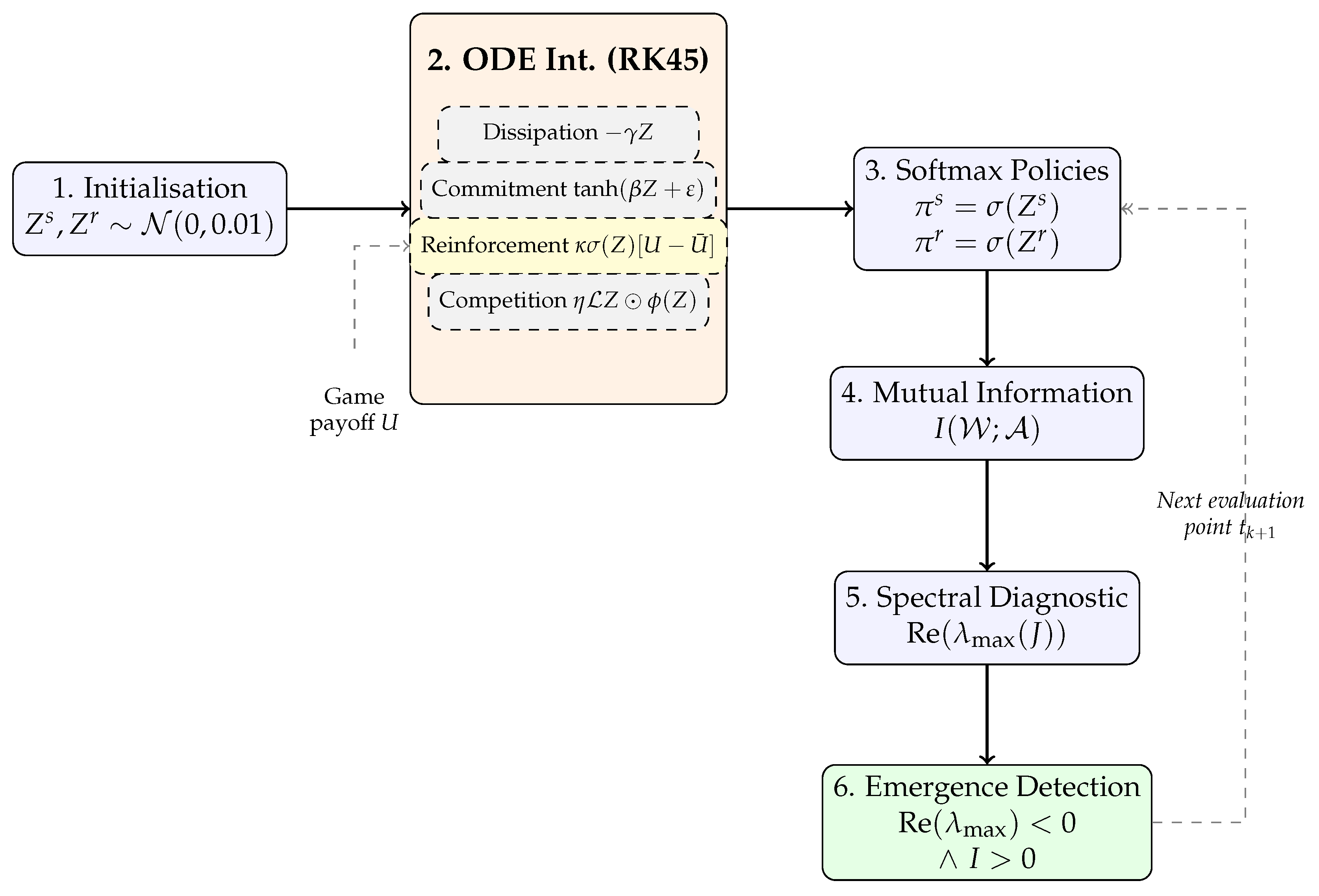
The experimental methodology follows the unified pipeline illustrated in Figure 1, which is described in Section 5.3.
All simulations are integrations (continuous in time, other than in Appendix E) of the belief dynamics (Equation (11)) on symmetric single-act Lewis signalling games. This study followed the unified pipeline illustrated in Figure 1. The following assumptions and parameters were used, unless otherwise stated.

5.1. Experimental Assumptions

Assumption 1
(Game structure). Symmetric Lewis signalling games are utilised with | W | = | M | = | A | = 3 and the payoff matrix U = I (identity), representing lossless coordination. The Markov chain structure is W M A . The The game is symmetric and general-sum; the unique optimal convention is a separating equilibrium with a one-to-one state–message–action mapping.
Assumption 2
(Laplacian structure). L row connects all logits sharing the same world-state index i (competition among messages for a given state), L col connects all logits sharing the same message index j (competition among states for a given message). This enforces unambiguous signalling conventions.
Assumption 3
(Policy parametrisation). Sender beliefs Z s R | W | × | M | and receiver beliefs Z r R | M | × | A | are initialised i.i.d. from N ( 0 , 0.01 ) to break the exact symmetry.
Assumption 4
(Dynamics parameters). The ODE (11) is integrated with the Dormand–Prince method (RK45) with absolute tolerance 10 9 and relative tolerance 10 6 over the horizon T = 100 . All parameters are listed in Table A1, which serves as a single authoritative reference.
Equation (11) is a continuous time ODE, Z ˙ = f ( Z ) . It is integrated over a fixed horizon T = 100 of continuous time. When reporting, the trajectory was sampled at uniform time intervals Δ t = 1 , giving K = T Δ t = 100 evaluation units. Each point is indexed as episode k = 0 , , K . Each evaluation point corresponds to a continuous time t = k Δ t [ 0 ; T ] . The internal adaptive step size of the integrator is independent of the reported grid.
Assumption 5
(Implementation). The curves show the mean over n = 20 independent random seeds. The shaded regions indicate ± 1 standard deviation. The leading eigenvalue Re ( λ max ) is numerically computed from the Jacobian of the full joint system at each time step.
The experiments are based on an OpenSpiel [43] implementation of Lewis’s signalling games. The goal of this study is to highlight the theoretical analysis and show its limitations. A direct comparison with neural communication architectures is not viable because of the policy-class mismatch: neural networks lack an explicit low-dimensional belief state Z whose Jacobian spectrum can be tracked.
The parameter window is chosen to satisfy the clean bifurcation regime as follows:
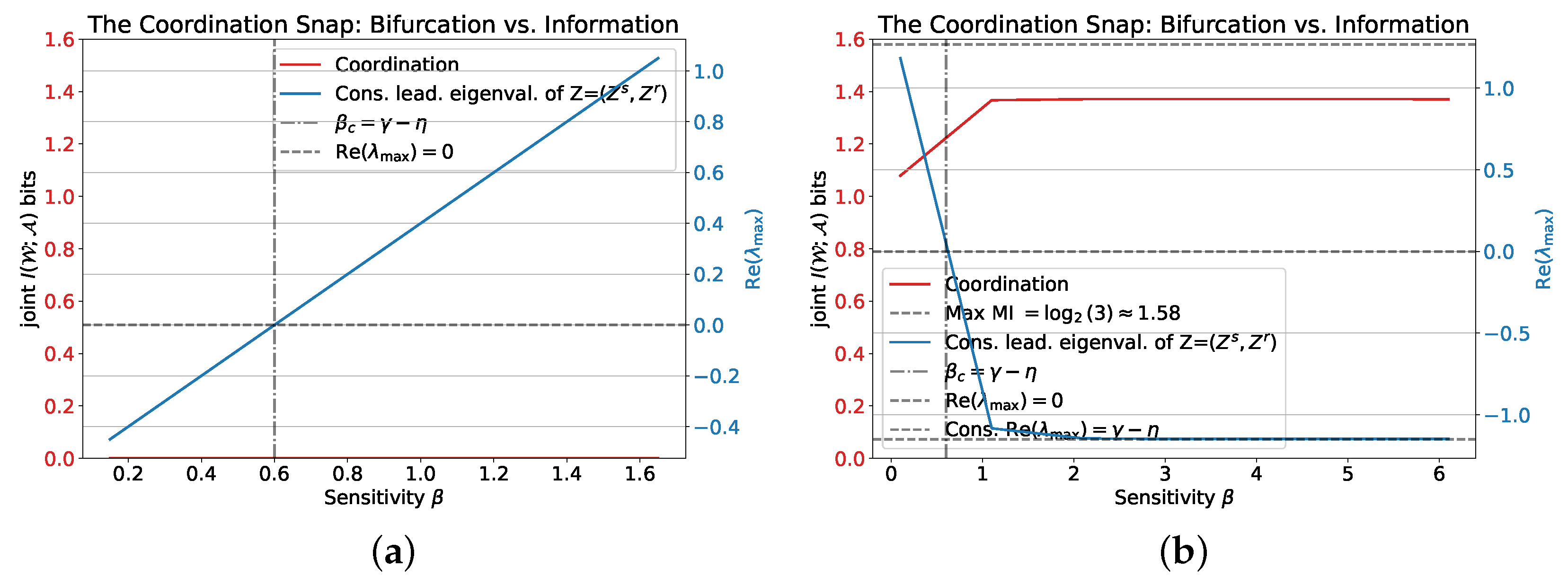
β c < β , where β c = γ ( n 2 ) η = 1.15 ( 3 2 ) 0.55 = 0.6 .
For the parameters in Table A1, β = 2.0 > β c = 0.6 , ensuring the consensus mode is unstable and the system undergoes a supercritical pitchfork bifurcation.

5.2. Simulation Metrics

All metrics are computed at each evaluation point t k = k Δ t with Δ t = 1 , k = 0 , , K and K = T / Δ t = 100 . The explicit formulas are provided below for reproducibility.
Mutual Information. The end-to-end Mutual Information I ( W ; A ) is computed from the joint distribution p ( w , a ) = m M p ( w ) π s ( m | w ) π r ( a | m ) :
I ( W ; A ) = w p ( w ) log 2 p ( w ) a p ( a ) log 2 p ( a ) + w , a p ( w , a ) log 2 p ( w , a ) .
NashConv. Following [43], NashConv is the sum of each agent’s improvement from unilateral deviation:
NashConv ( π s , π r ) = i { s , r } max π i U i ( π i , π i ) U i ( π i , π i ) ,
where U i is the expected utility for agent i and the best response is is computed by an exhaustive search over deterministic policies.
Coordination Success. The percentage of optimal actions is
Success = 1 | W | w W I arg max a π r a | arg max m π s ( m | w ) = w × 100 % .
Emergence Time. The time to reach 90% of the maximum Mutual Information:
t emerg = min t k : Re ( λ max ( t k ) ) = 0 I ( W ; A ) > 0 .
If the threshold is never reached, t emerg = NA (not applicable).
Causal Influence of Communication (CIC). Following Lowe et al. [14],
CIC = E w p ( w ) D KL π r ( a | m ) P ( a ) , P ( a ) = m p ( m ) π r ( a | m ) .
This metric can be viewed as the degree to which a speaker’s message acts as a direct driver for changes in a receiver’s belief state or subsequent actions.

5.3. Methodological Pipeline

The pipeline shown in Figure 1 comprises the following stages:
  • Initialisation. Sender and receiver belief matrices Z s R | W | × | M | and Z r R | M | × | A | are initialised i.i.d. from N ( 0 , 0.01 ) to break exact symmetry (Assumption 3).
  • ODE Integration. The belief dynamics (Equation (11)) are integrated continuously via the Dormand–Prince method (RK45) with adaptive step size ( atol = 10 9 , rtol = 10 6 ) over horizon T = 100 (Assumption 5).
  • Softmax Policies. At each evaluation point t k = k Δ t ( Δ t = 1 , k = 0 , , K , K = 100 ), the belief matrices are converted to stochastic policies via the softmax function: π s ( m | w ) = σ ( Z s ) w m and π r ( a | m ) = σ ( Z r ) m a .
  • Jacobian Computation. The Jacobian J = f / Z of the full joint system is evaluated numerically at each time step (Assumption 5).
  • Eigenvalue Diagnostic. The leading eigenvalue λ max ( J ) is extracted; its real part Re ( λ max ) serves as the real-time detector of the emergence point (Theorem 1, Remark 3).
  • Mutual Information Calculation and Emergence Detection. The end-to-end Mutual Information I ( W ; A ) is computed from the joint distribution p ( w , a ) = p ( w ) m π s ( m | w ) π r ( a | m ) (Section 5.2). Communication emergence is declared at the first episode t k where Re ( λ max ( t k ) ) < 0 and I ( W ; A ) > 0 .
This pipeline is executed identically for all parameter sweeps ( β , γ , η , κ ) and for the Lewis game (33). The neural bridge experiment (Appendix E) replaces steps 2–3 with discrete gradient descent on the VFE potential while retaining the spectral diagnostic (steps 5–6).

5.4. Discussion on the Role of Nonlinearity

Behavioural patterns are verified at the origin ( Z = 0 ) and at an equilibrium ( Z 0 ) stage specified in Theorem 1. The results are demonstrated on a classic example of a 3-state Lewis Signalling game [11] whose payoff matrix is
1 0 0 0 1 0 0 0 1 .
This game describes trivial communication channels.
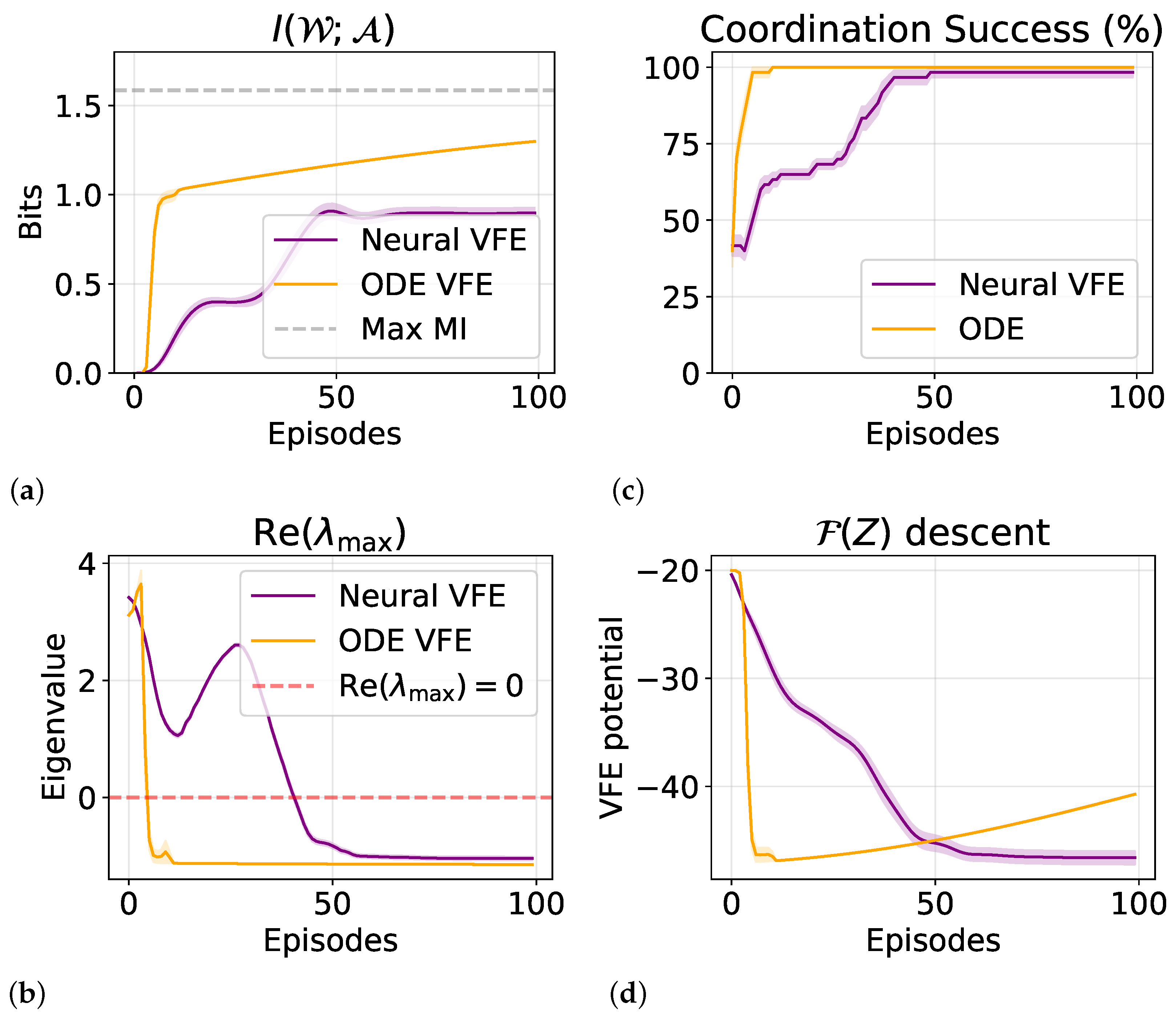
The results are shown in Figure 2. At the origin (left), the leading eigenvalues experience a discontinuous transition at β c = γ ( 3 2 ) η = 0.6 above the bifurcation. (as per Remark 4) that correspond to the switch of the system’s behavioural state from babbling. I ( W ; A ) also experiences a small snap, approximately 10 6 . Subsequently, as | Z | grows with the system evolution, the latter establishes a stable convention matching the stability conditions of the theorem: I ( W ; A ) reaches around the critical value of log 2 3 1.37 ± 0.02 bits, and Re ( λ max ) turns negative, plateauing at γ = 1.15 confirming Theorem 1. It was also found that sometimes the agents can “jump out” of the convention and return, which is not proven formally but shows the non-stationarity of the process. At equilibrium, the Mutual Information is dominated by the dissipation dictated by the coefficient γ , establishing a stable condition, whereas the leading eigenvalues exponentially converge to a stable state of imperfect communication.
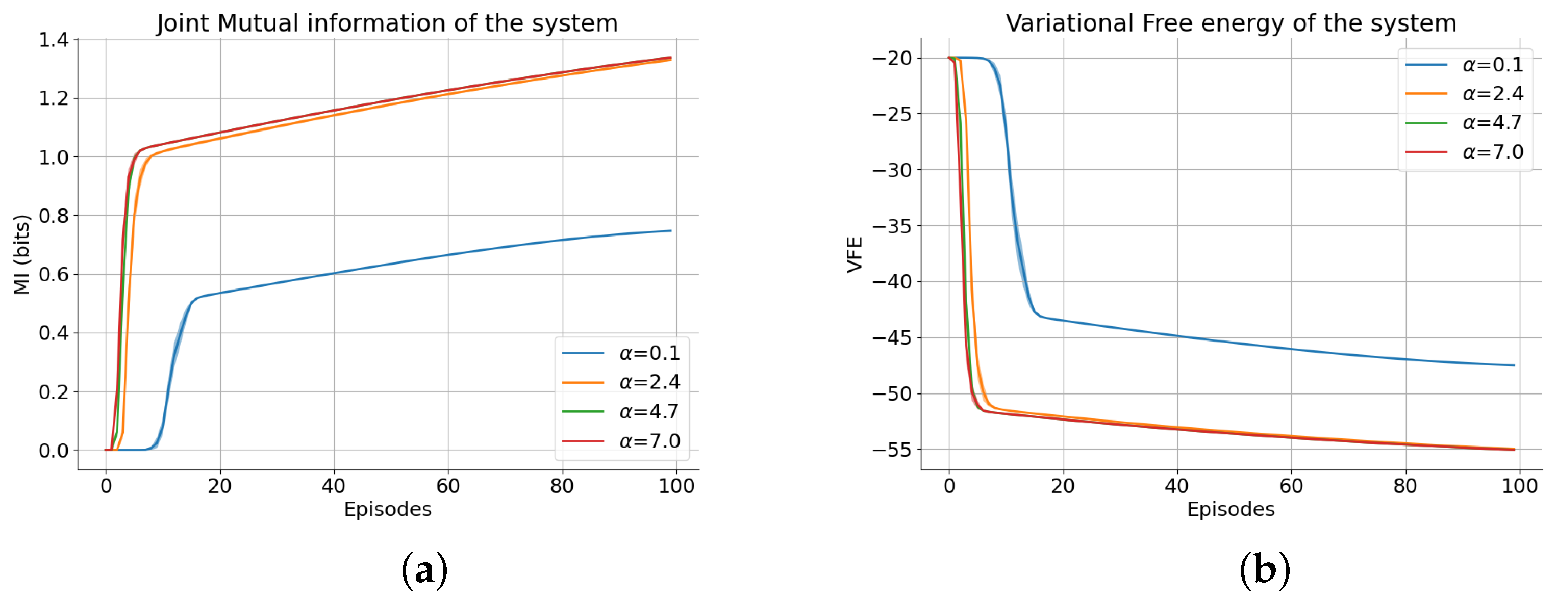
In addition, the equivalence of the two objectives considered in this study was empirically visualised. As shown in Figure 3, for different values of β , maximising I ( W ; A ) corresponds to minimising the VFE. However, in practice, it was observed that for some β that do not satisfy Theorem (iii), for instance, β = 0.1 ( β < γ ), the equivalence does not follow, and the system does not achieve high Mutual Information. For more metrics and analyses of the Lewis game, refer to Appendix C.2.
This validates the theoretical framework: the emergence of meaning in challenging environments is not merely a function of reward maximisation but a delicate balance of damping-induced stability within the VFE potential. Moreover, the nonlinear parameter dependence is instrumental in establishing emerging behavioural patterns.

5.5. Discussion on the Role of Dissipation

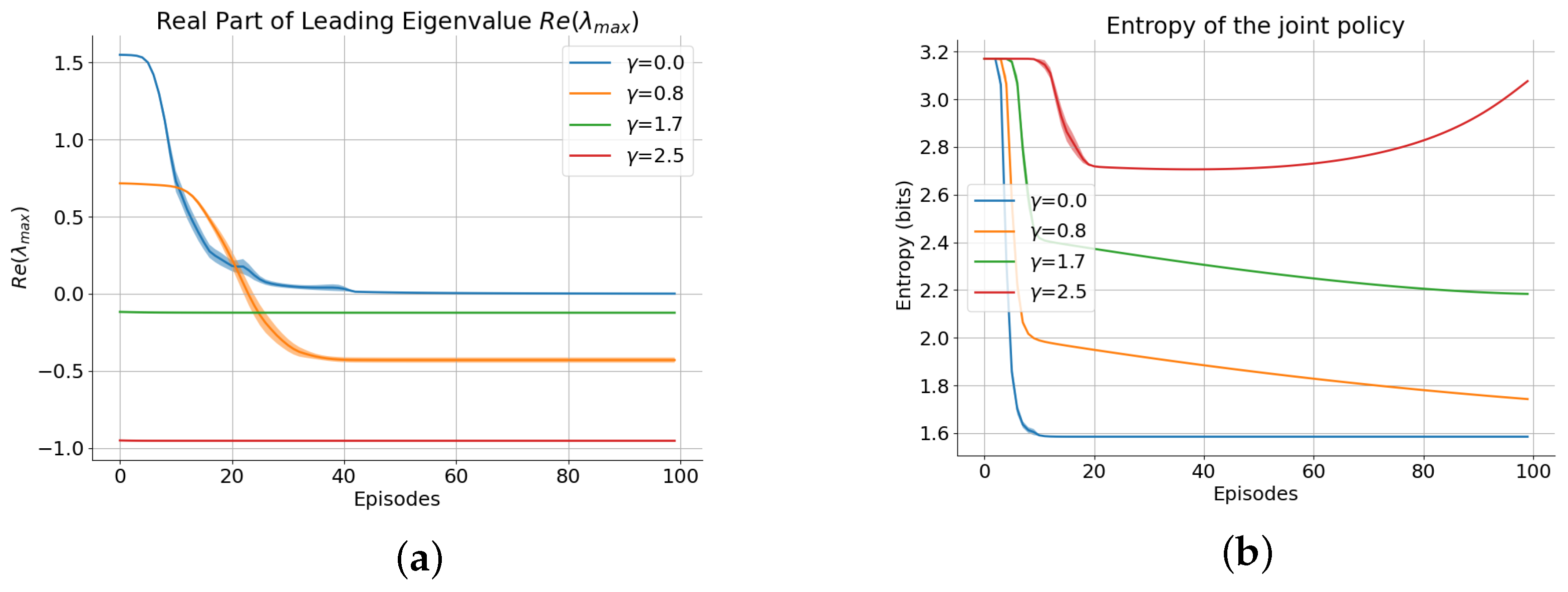
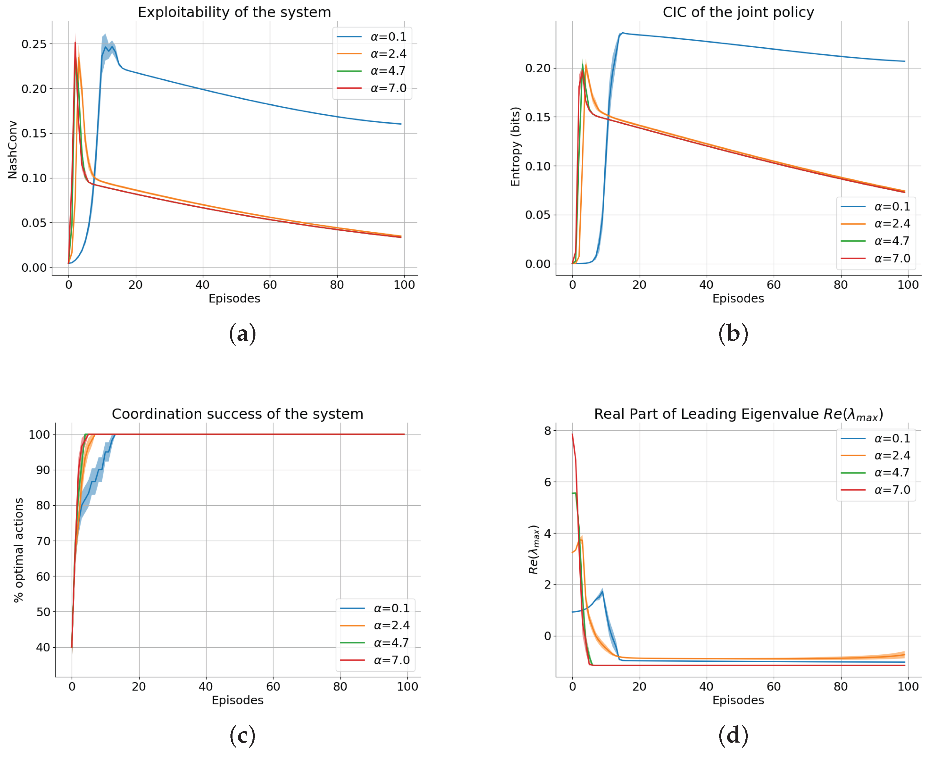
While the reinforcement and commitment terms of Equation (11) drive its evolution, the dissipation term is supposed to act like a regulariser, stabilising the model. However, the Lewis coordination game, being a potential game, allows convergence to a Nash equilibrium even without explicit dissipation. By varying γ while holding other terms fixed, it was possible to effectively interpolate between the standard absence of regularisation ( γ 0 , conservative, cycle-prone) and the full VFE descent model ( γ > 0 , convergent), as demonstrated in Figure 4.
To investigate the effect of dissipation on convergence, simulations were performed with varying γ values, while holding the other parameters fixed. The resulting convergence metrics are summarised in Table 3.
The numerical results are presented in Table 3. Over-regularised ( γ = 4.5 ) or unregularised cases do not achieve any emergent behaviour (they maintain a good level of coordination, achieving the game gradient alone, not through spectral decay) during simulation. The only value of γ that yields non-zero Mutual Information is γ = 0.8 < 2.0 = β which satisfies Theorem 1. Even in the example of the Lewis coordination game, without dissipation, the system 11 can be stuck in chaotic stable ( γ = 4.5 ) unstable ( γ = 0 ) states, keeping the eigenvalues either spiralling out of control or plateauing. Higher γ values reduce the final Mutual Information (as the system is pulled toward the high-entropy origin) while still achieving perfect coordination success.

5.6. Roles of Connectivity and Reinforcement

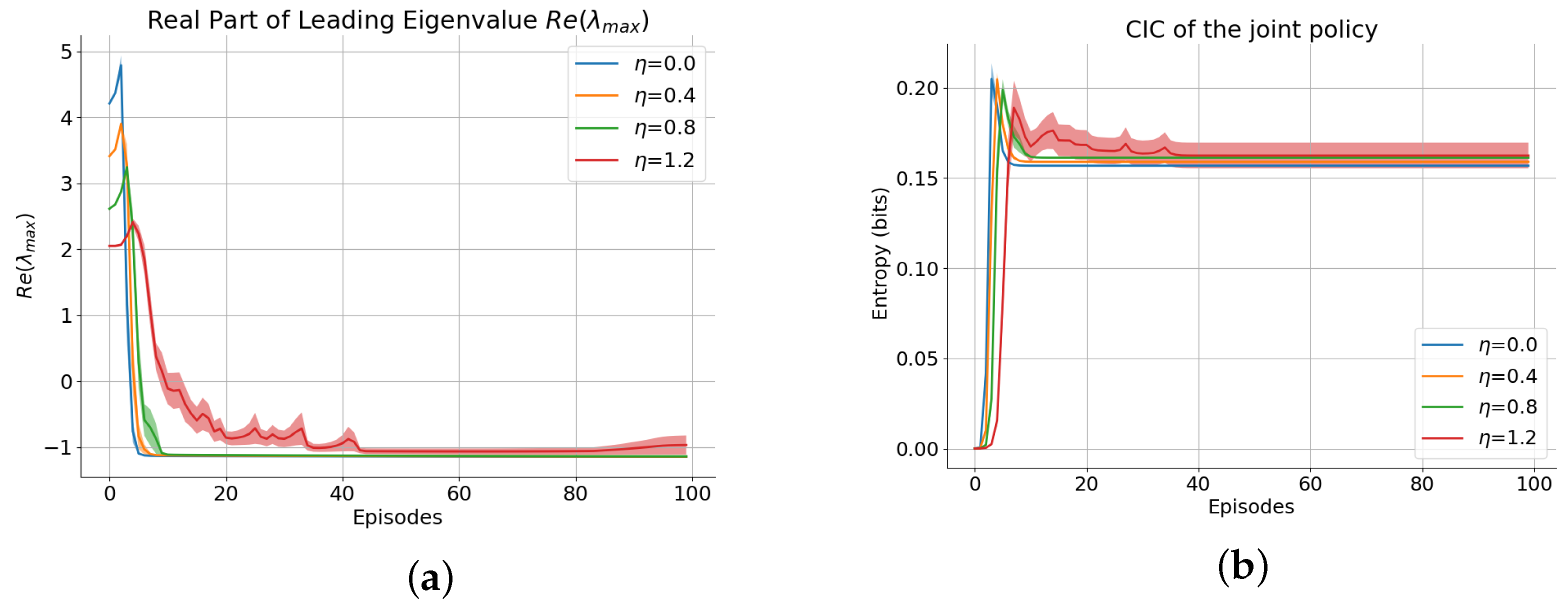
The effects of connectivity and reinforcement on the system dynamics are illustrated in Figure 5 and Figure 6, respectively. The communication topology regularisation η L Z ϕ ( Z ) was verified and was consistent with Remark 2. Across all tested values of η , the system reached a stable CIC of approximately 0.2 ± 0.03 (Figure 5, right). However, an excessively large η (e.g., 1.2 ) slows the convergence and increases the variance, as shown in Table 4.
The numerical results are presented in Table 4. The results are consistent with empirical evidence. However, the question of how the agent topology impacts regularisation remains open and is left for future research.
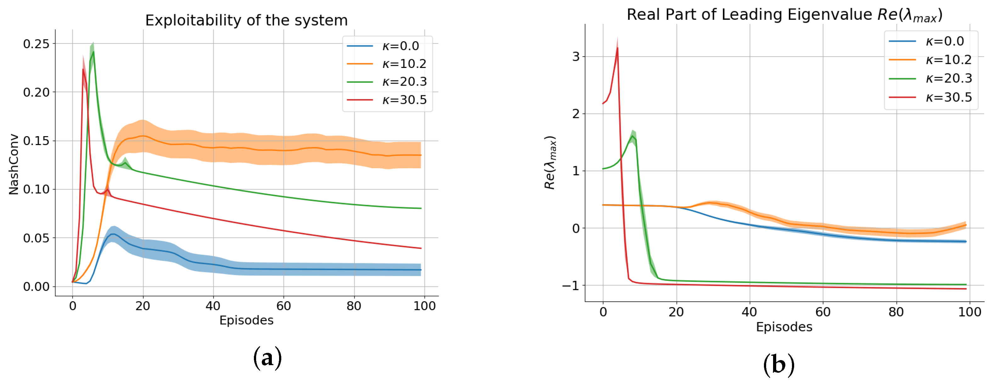
The separate influence of the reinforcement coefficient κ is shown in Figure 6.
The reinforcement coefficient κ governs the payoff-driven component of the belief dynamics. Table 5 presents the impact on the convergence metrics and coordination success.
The separate influence of the reinforcement coefficient κ on the system’s evolution can be observed in Figure 6. It helps drive cooperation in the system, steadily increasing the agent’s Mutual Information (left) and increasing the success rate of establishing communication (centre). Notably, the agents were unable to communicate successfully in 33 % of scenarios when κ = 0 and the dependency was monotone, as can be deduced from the quantitative evaluation in Table 5. This implies a clear distinction between the reinforcement and commitment terms: the latter served as the main learning force of the system, while the former provided the emergence mechanism through the bifurcation property (Theorem 1).
Remark 7
(Note on coordination success vs. communication emergence). A high coordination success can arise from degenerate or constant policies without meaningful signalling. For example, if the sender always emits the same message and the receiver always takes the same action, coordination success may be high (if the action happens to match the state), while I ( W ; A ) 0 . Therefore, coordination success alone is not a reliable indicator of communication emergence, I ( W ; A ) > 0 is the definitive diagnostic. This explains the apparent discrepancy in Table 3.

5.7. Sensitivity Analysis

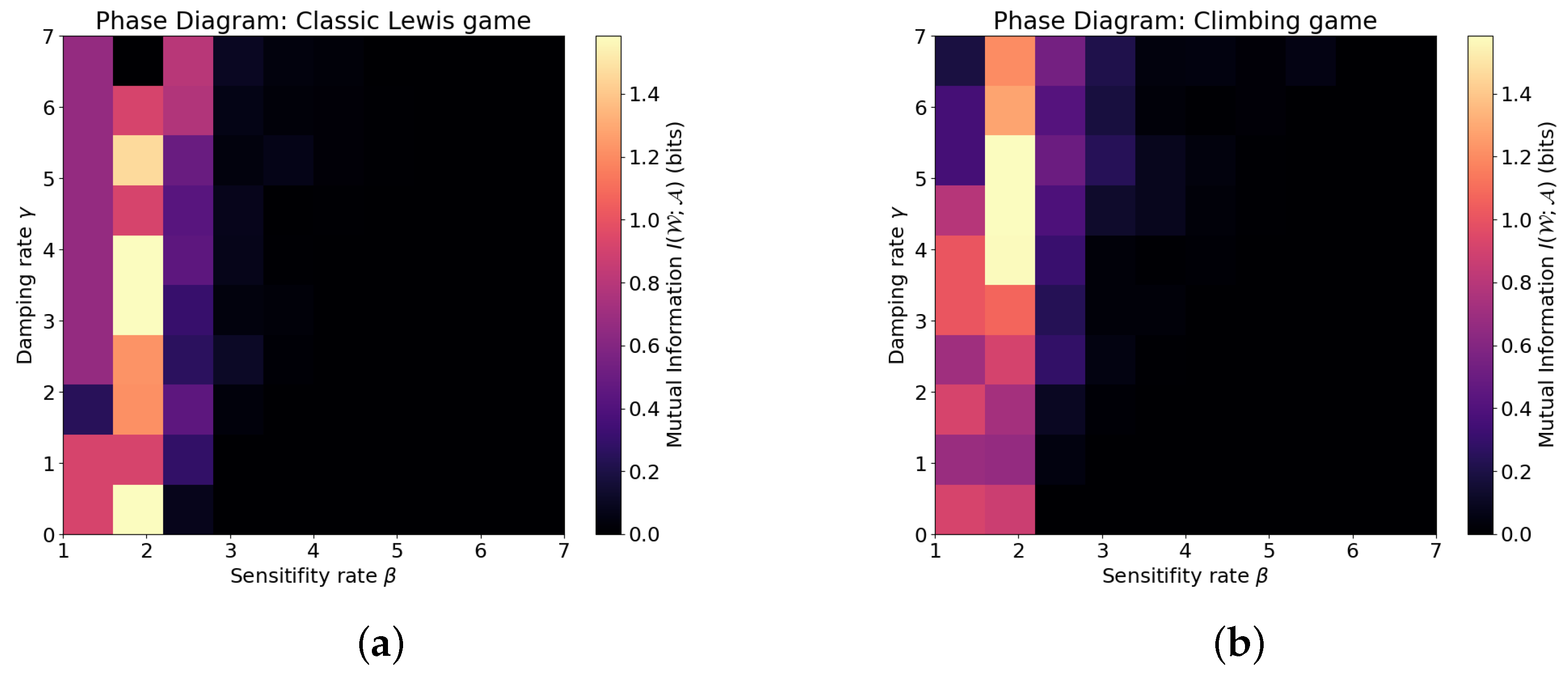
Phase analysis is performed (Figure 7) for the Lewis game (33) and the Climbing Game [44] (a 3 × 3 game characterised by a high-payoff attractor surrounded by severe penalties for miscoordination) shows that there are parameter regions that have high Mutual Information and large fields of non-useful parameter combinations in the neighbourhood of the origin, which agrees with the theoretical and empirical results obtained above. Nevertheless, this implies that even for the system (11) which has a low number of parameters, there is a need to further investigate how to derive stable parameter regions and how to scale the method to multiparametric models. The latter was chosen to be left for future work.

5.8. Bridge to Neural Networks

The spectral diagnostic of Theorem 1 requires an explicit belief matrix Z and a closed-form or numerically tractable Jacobian matrix. Generic deep multi-agent policies, parameterised by high-dimensional neural networks, do not necessarily possess such a property; thus, the exact threshold μ = 0 cannot be extracted from black box agents. However, the underlying dynamical mechanism, a supercritical pitchfork bifurcation driven by the competition between sensitivity and dissipation, predicts a universal signature; a sharp transition from near-zero Mutual Information to a stable signalling convention once an effective learning characteristic (leading eigenvalue) crosses a critical value. In Appendix E, it is verified that this signature appears even when the commitment nonlinearity is replaced by a small MLP that is updated via an algorithm conceptually aligned with Neural Replicator Dynamics [21]. The quantitative results are presented in Table 6. As the method demonstrates worse results in principle (other than the emergence time), it generally follows the established theoretical framework. While the exact spectral diagnostic requires an explicit low-dimensional belief state Z, the evaluation shows that the same sharp MI transition emerges in a neural network trained by discrete VFE descent on the Lewis signalling game. The leading eigenvalue of the ODE Jacobian, evaluated at the output logits of the network, tracks the transition without continuous-time integration, suggesting that the bifurcation mechanism is not entirely an artefact of ODE formalism.

6. Conclusions and Future Work

A recurring challenge in multi-agent reinforcement learning (MARL) is its explainability; agents fail to coordinate because they never receive the reward signal required to break the symmetry of random babbling. Conventionally, this tends to be mitigated through “trial-and-error” procedures, such as reward shaping of extensive hyperparameter tuning or post hoc methods that attempt to perform credit assignment of the policies. This study, on the other hand, provides an analytical alternative based on an explicit parameterised model of continuous nonlinear system dynamics that enables the identification of the conditions for meaning to emerge, paving the way for a dynamical analysis of agentic systems.
This study provides two results for the analysis of the topological transition point of emerging communication. First, the leading eigenvalue λ max provides a formal reasonable indicator for the moment of the emerging meaning, as shown in Theorem 1. In a signalling game, the period where λ max > 0 corresponds to a state of active negotiation. During this phase, the agents occupy an unstable manifold where the zero-information pooling equilibrium is shattered, but a stable convention has not yet been reached. The sudden drop in VFE and the spike in joint Mutual Information occur precisely when the system finds a stable communication sink ( λ max < 0 ). This negative eigenvalue serves as a stability measure, ensuring that the convention resists environmental noise. The eigenvalue serves as a measure of the signalling equilibrium convergence. Moreover, cyclic behaviour may be observed, depending on the presence of dissipation in the system for its various topologies, as demonstrated in Theorem 2. The findings were experimentally validated for different types of symmetric signalling games. Moreover, a toy neural example demonstrated that the analysis could be potentially applied to neural networks with a small number of hidden neurones.

Limitations and Future Work

The neural experiment in Appendix E is presented as a phenomenological observation in a small, low-dimensional setting. Importantly, this demonstrates that the qualitative bifurcation signature (a sharp transition from near-zero Mutual Information to stable signalling) is observable when the commitment nonlinearity is implemented by a small MLP trained by gradient descent. However, it does not validate Theorems 1 and 2 for general deep reinforcement learning policies, where the spectral diagnostic requires an explicit low-dimensional belief state Z whose Jacobian spectrum can be computed in closed form. Moreover, scalability to large vocabularies, many agents, or partial observability remains unproven.
However, this opens the door for investigating state-of-the-art deep learning models that have many more parameters and can be more robust to initialisation. They can help incorporate the spatiotemporal dynamics of the game using, for example, neural network-based ODEs or generative models based on diffusion or flow matching [45]. Even with different numbers of parameters, the spectral analysis tools introduced above can be applied. The criticality condition from [12] β · λ max ( A ) > γ implies that a communication protocol requires a constant “flow” of commitment force ( β ) caused by the agents’ strive to reach the goal while remaining stable against the natural decay of information ( γ ). This creates an opportunity to apply probabilistic methods and methods simulating decision-making, such as the evolution of a dynamic system (see, for example, ref. [46]). Their spectral sensitivity analysis, based on the Jacobian-vector product, allows for this new view of meaning emergence to challenge the static and purely empirical perspective of conventional MARL, suggesting that communication is a constant adaptive process. Additionally, it motivates the search for multiple bifurcations and, consequentially, the consideration of more stages of communication and their stability in large-scale multi-agent systems inspired by progress in self-organising systems research.

Author Contributions

Conceptualization, I.T., A.C., N.G. and A.V.; methodology, A.C.; software, A.C.; validation, I.T. and A.C.; formal analysis, I.T., A.C. and N.G.; investigation, all authors; writing—original draft preparation, A.C.; writing—review and editing, all authors; visualisation, A.C.; supervision, A.V. All authors have read and agreed to the published version of the manuscript.

Funding

This work was supported by the Ministry of Economic Development of the Russian Federation (IGK 000000C313925P4C0002), agreement No. 139-15-2025-010.

Institutional Review Board Statement

Ethical review and approval were waived for this study because it used publicly available benchmark datasets and did not involve the new collection of human or animal data by the authors.

Informed Consent Statement

Not applicable.

Data Availability Statement

The source code for all simulations, including hyperparameter manifests (YAML), random seeds, solver configurations, and figure-generation scripts, is publicly available at https://github.com/alexunderch/vfe-emergent-bifurcation under the commit hash 59ba6cd1379e (https://github.com/alexunderch/vfe-emergent-bifurcation/blob/c81994918a2272e2498a13cd9a8459ba6cd1379e). The repository includes a README-file (https://github.com/alexunderch/vfe-emergent-bifurcation/blob/c81994918a2272e2498a13cd9a8459ba6cd1379e/README.md) that contains installation instructions, software library versions, and a single-command-line script that regenerates all figures and tables in the manuscript. To facilitate full reproducibility, the following checklist was provided: Software versions: Python >= 3.12; NumPy == 2.3.5; SciPy == 1.17.0; Matplotlib == 3.10.8; Pandas = 3.0.0; OpenSpiel == 1.16.11, Jax == 0.9.0.1 (comp. modelling, neural bridge), and Diffrax == 0.7.1 (ODE modelling); Random seeds: 20 independent seeds (0–19) are hard-coded in src/experiment.py; Hyperparameter manifests: All parameters are stored in src/experiment.py; Expected output files: Running the main script produces results/containing (i) trajectory logs (traj_{game}_param{i}.txt), (ii) convergence metrics (metrics_{game}_table.csv), and (iii) figure PDFs (fig_{game}_*.pdf) identical to those in this manuscript; Exact verification command: python src/experiment.py. The repository was accessed on 5 July 2026.

Acknowledgments

The authors thank the maintainers of the public benchmark datasets and the open-source software used in the experiments.

Conflicts of Interest

The authors declare no conflicts of interest.

Appendix A. Variational Free Energy Derivations

Appendix A.1. Probabilistic Version

The sender’s VFE is derived in full, and the receiver follows by analogy.
  • Step 1. Generative model.
An auxiliary binary optimality variable O , where O = 1 denotes that the joint action is optimal. The probability of optimality given state w W and action a A is
p ( O = 1 w , a ) = exp κ U ( w , a ) ,
where κ is an inverse-temperature parameter that scales the rationality of the system.
The generative model for an optimal trajectory is
p ( m , a , O = 1 w ) = P ( m ) P ( a m ) p ( O = 1 w , a ) ,
where P ( m ) is the prior over messages, and P ( a m ) is the prior over actions given a message.
  • Step 2. Variational joint policy.
The agents use a parameterised joint policy defined by the Markov chain W M A :
q ( m , a w ) = π s ( m w ) π r ( a m ) .
  • Step 3. KL divergence (global identity).
The VFE is the expected KL divergence between the variational policy and optimal generative model:
F = E p ( w ) D KL q ( m , a w ) p ( m , a , O = 1 w ) .
Expanding the logarithm of the ratio:
F = w p ( w ) m , a π s ( m w ) π r ( a m ) log π s ( m w ) π r ( a m ) P ( m ) P ( a m ) exp ( κ U ( w , a ) ) = w p ( w ) m π s ( m w ) log π s ( m w ) P ( m ) ( i ) Sender KL + w , m p ( w ) π s ( m w ) a π r ( a m ) log π r ( a m ) P ( a m ) ( ii ) Receiver KL κ w , m , a p ( w ) π s ( m w ) π r ( a m ) U ( w , a ) ( iii ) Expected utility .
  • Step 4. Receiver prior assumption.
To isolate the communicative bottleneck, it can be assumed that the receiver’s prior matches its policy: P ( a m ) = π r ( a m ) . Then, term (ii) vanishes because log 1 = 0 . Recognising that a π r ( a m ) = 1 , term (i) simplifies exactly to the Mutual Information I ( W ; M ) . Term (iii) is the expected utility E Π [ U ] .

Appendix A.2. Joint VFE Bound

By summing the two functionals and applying the chain rule for MI on the Markov chain W M A :
I ( W ; M ) = I ( W ; A ) + I ( W ; M A ) ,
I ( M ; A ) = I ( W ; A ) + I ( M ; A W ) .
Therefore,
F tot = F s + F r = 2 κ E [ U ] ( 2 I ( W ; A ) + I ( W ; M A ) + I ( M ; A W ) ) .
Dividing by 2 and moving terms to the maximisation side gives Lemma 1:
min π s , π r F tot = max π s , π r E [ U ] I ( W ; A ) + L , L = 1 2 I ( W ; M A ) + I ( M ; A W ) .

Appendix A.3. Dynamical Vision

Notably, there exists an infinite number of potentials for the same dynamics. One of these suits the definition.
Because the dynamics (11) are additive, the Free Energy function F can also be decomposed into a sum of the following terms:
F = Φ decay + Φ commitment + Φ L + Φ feedback .
  • Complexity/Decay ( Φ decay ) could be obtained by integrating γ z what gives the quadratic “cost of belief”: Φ decay = γ 2 z 2 + const .
  • Inference Drive/Commitment ( Φ commitment ) is an integral of tanh ( β z + ϵ ) , which yields the Log-Cosh potential: Φ commitment = 1 β ln ( cosh ( β z + ϵ ) ) + const ( ε ) .
  • Competition ( Φ L ): Since the Laplacian inhibition is a linear operator on z, it acts like a smoothing or “repulsion” energy yielding a quadratic form Φ L = η 2 z T L z .
  • Extrinsic Value/payoff ( Φ feedback ): the “reinforce’-like term uses the policy gradient ( I π ) . This is the gradient of the log-likelihood policy. Thus, the payoff potential is a negative expected payoff.
Let us derive the latter using backward induction. The expected utility for a message–action pair is U = j σ ( Z ) j U j . It takes the gradient with respect to the i-th logit Z i :
U Z i = j U j softmax ( Z ) j Z i
Using the property of the softmax derivative, σ j Z i = σ i ( δ i j σ j ) , it follows that
U Z i = U i σ i ( Z ) σ i ( Z ) j σ j ( Z ) U j
Factoring out the softmax term:
Z i U = σ i ( Z ) U i U ¯
where U ¯ = j σ j ( Z ) U j is the mean utility currently expected by the agent, and This is the “Replicator”-like term: the logit Z i grows if its associated payoff U i is better than the current average, reinforcing it to obtain higher payoffs.

Appendix B. Information Geometry of the Policy Simplex

The derivations in this appendix are standard and are included for completeness. For geometric foundations, see Amari (1998) [37] and Harper (2009) [39].
Lemma A1
(Softmax Jacobian and Fisher Metric). Let π ( z ) = σ ( z ) be the softmax policy and let
J π ( z ) = π z = diag ( π ) π π .
Let g ( π ) be the Shahshahani [39,47] metric g i j ( π ) = δ i j / π i on the probability simplex Δ n , restricted to tangent vectors δ π satisfying i δ π i = 0 . Then
J π ( z ) = g ( π ) 1 | T Δ n .
Proof. 
The Fisher information matrix for the categorical distribution is
I i j ( π ) = E log p π i log p π j = δ i j π i .
On the tangent space of the simplex, the inverse of this diagonal matrix is exactly diag ( π ) π π , which is J π . □
Lemma A2
(Natural Gradient Identity). Let V ( π ) be a smooth function on Δ n and let V ˜ ( z ) = V ( σ ( z ) ) . The natural gradient of V with respect to π equals the Euclidean gradient of V ˜ with respect to z
z V ˜ ( z ) = J π ( z ) π V ( π ) = g 1 ( π ) π V ( π ) = ˜ π V ( π ) .
Proof. 
By the chain rule,
z V ˜ = π z π V = J π π V .
Because J π is symmetric ( J π = J π , a consequence of the softmax being a gradient map of the log-sum-exp function), it obtains z V ˜ = J π π V . By Lemma A1, J π = g 1 , which is the defining relation of the natural gradient. □
Lemma A3
(Alignment with Mutual Information). Let V ( π ) = F ( π ) where F is the Variational Free Energy. At the babbling equilibrium Z = 0 , the principal eigenvector of J π | Z = 0 is collinear with the natural gradient of the Mutual Information I ( W ; A ) .
Proof. 
At Z = 0 , π is uniform, thus J π | 0 = 1 n ( I 1 n 1 1 ) . This matrix is projected onto the tangent space of the simplex. The Hessian of the KL divergence (and hence of F ) at the uniform point is proportional to the Fisher information matrix, whose leading eigenvector identifies the direction of the steepest increase in Mutual Information. By Lemma A2, the Euclidean gradient z V coincides with the natural gradient. □

Appendix C. Experimental Details

Appendix C.1. Parameters

Table A1. Description of the system parameters used in the experiments (Equation (11)). The solver was the Dormand-Prince Runge-Kutta method (RK45) with adaptive time-stepping. All parameters are dimensionless aside from Mutual Information measured in bits. N ( μ , σ 2 ) denotes the normal distribution.
ParameterSymbolValueMeaning /Justification
Sensitivity β 2.0Gain on evidence; set above critical threshold β c = γ ( n 2 ) η to ensure bifurcation
Damping/dissipation γ 1.15Forgetting rate, anchors system to high-entropy origin; chosen to satisfy β c = γ ( n 2 ) η for stability at equilibrium
Symmetry-breaking bias ε 0.025Small perturbation to prevent perfect trapping at Z = 0 ; standard in pitchfork analysis
Reinforcement gain κ 30.0Scales payoff gradient; kept small that commitment ( β ) and dissipation ( γ ) dominate the transient
Laplacian inhibition η 0.55Enforces one-to-one mappings, tuned to penalise ambiguous conventions without preventing convergence
SolverRK45 (ODE45)Based on the explicit Runge-Kutta Dormand-Prince (4,5) method, it uses adaptive time-stepping to balance computation speed with atol = 10 9 and rtol = 10 6 .
HorizonT100Total continuous time units. Sufficient for transient decay and equilibrium approach
Reporting grid Δ t 1Uniform episode dividing time interval.
Number of episodesK100 K = T Δ t evaluation points.
Integrator step sizeAdaptivecontrolled by the integrator. Initial value is 0.01
Random seeds20 independentReported as mean ± std. in shaded regions
Initialisation Z 0 N ( 0 , 0.01 ) Small noise around a babbling equilibrium
The empirical (Figure A1) and theoretical results (Table A2) are analysed.
The parameters used in the experiments are listed in Table A1. Additionally, phase diagrams and sweeps were performed on the following grids:
  • Sensitivity sweep ( β ): from 1 to 10, 100 uniform points;
  • Dissipation sweep ( γ ): from 0 to 7, 100 uniform points.
  • Integration per grid point: t [ 0 ; T ] .

Appendix C.2. Additional Evaluations

Figure A1. Parametric plots for the Lewis signalling game over 100 episodes for different values of β . (a) Exploitability (NashConv). (b) Coordination success (percentage of optimal actions). (c) Real part of the leading eigenvalue. Re ( λ max ) . (d) Mutual Information I ( W ; A ) (bits). Curves show mean over 20 seeds; shaded regions indicate ± 1 standard deviation. Other parameters as in Table A1.
Technologies 14 00432 g0a1
Table A2. β -sweep simulation results for the Lewis signalling game. The metrics are defined in Table 3. Values are mean ± standard deviation over 20 seeds. Parameters: γ = 1.15 , η = 0.55 , κ = 30.0 , ε = 0.025 .
Parameter β NashConvRe( λ max ) I ( W ; A ) Coord. SuccessEmerg. Time
0.10.09 ± 0.00−1.09 ± 0.001.02 ± 0.00100.00 ± 0.008.40 ± 0.27
2.40.04 ± 0.00−1.15 ± 0.001.30 ± 0.00100.00 ± 0.003.45 ± 0.20
4.70.04 ± 0.00−1.15 ± 0.001.30 ± 0.00100.00 ± 0.002.65 ± 0.22
7.00.04 ± 0.00−1.15 ± 0.001.30 ± 0.00100.00 ± 0.002.65 ± 0.29

Appendix C.3. Exploitability (NashConv)

Across all β values, the system moves closer to a Nash Equilibrium as training progresses. The lowest value ( β = 0.1 ) rises much slower but settles around the same exploitability; however, it does not go through the emergence phase. Learning dynamics actively drive agents into exploitable non-equilibrium states. Higher β accelerates this divergence and traps the agents in a worse configuration, and a very low β cannot cause any emergent behaviour at all.

Appendix C.4. Coordination Success (% Optimal Actions)

The higher β runs 4.7 , 7.0 show a rapid initial spike in coordination (hitting 95–100% quickly), followed by a plateau of low variance outcome. Conversely, β = 0.1 shows a slow, steady climb, ultimately reaching a slightly lower ( 98.33 ± 1.67 %) with a larger variance. A high β induces premature convergence. The agents quickly switch to a partial coordination scheme that eventually succeeds; however, it can also break down in the case of more sophisticated strategy landscapes. A lower β allows for a slower and more robust exploration phase, leading to a stable and successful joint policy.

Appendix C.5. CIC of the Joint Policy

A high β creates a steeply sloped dynamic landscape that forces the system into a local minimum. Once the eigenvalue crosses zero (approximately episode 10), the system is locked into that attractor. Because it was forced there so quickly, the attractor landed in an exploitable region, causing the inability to extract valuable communication. However, as demonstrated above, the desired behaviour can be obtained with different regularisations. Even in Figure A1 in Appendix C, the CIC stabilises at approximately 0.10 ± 0.04 .

Appendix C.6. Leading Eigenvalue and Emergence Time Analysis

High β values start highly unstable but plummet rapidly, crossing the 0 threshold around episode 2 10 . A high β creates a steeply sloped dynamic landscape that violently forces the system into local minima.

Appendix C.7. Conclusions

β acts as a cooling commitment mechanism that drives behaviour. When β is high, it effectively over-stabilises the system. The eigenvalues rapidly decrease to below zero, trapping the agents in the nearest local minimum. This results in the rapid spikes and subsequent collapses seen in the early episodes, even though the policy is highly exploitable and sub-optimal. When β is low ( β = 1.0 ), the system remains mathematically fluid for the entire integration period ( R e ( λ m a x ) remains positive). This prolonged exploratory phase prevents them from being trapped in early local minima, allowing them to slowly discover a more robust, highly coordinated, and less exploitable policy.

Appendix D. Cubic Coefficient of the Center-Manifold Reduction

Appendix D.1. Setup and Notation

Let the joint belief vector be
Z = vec ( Z s ) vec ( Z r ) R D .
Set the bifurcation parameter μ = β γ + ( n 2 ) η and fix ε = 0 (the symmetry-breaking bias is treated as a perturbation in Remark 2). The dynamics (11) with vanishing reinforcement at the origin takes the form
Z ˙ = f ( Z ; μ ) = J ( μ ) Z + N ( Z ) + O ( Z 5 ) ,
where the linear part is
J ( μ ) = J 0 + μ I , J 0 = γ I + η L ϕ ( Z ) + β I + κ H U , β c = γ ( n 2 ) η
and N ( Z ) contains the nonlinear terms from the element-wise tanh saturation.
Remark A1
(Symmetric invariant subspace). In the full joint space, the Laplacian null space is at least two-dimensional (one constant mode for Z s and one for Z r ). The analysis is restricted to the symmetric invariant subspace  S = { Z s = Z r } , which is preserved when the payoff matrix U is symmetric and both agents share identical initial conditions. On S the two constant modes collapse to a single eigenvector; therefore, the critical eigenvalue λ c is simple. The centre-manifold reduction is one-dimensional.
Specifically, the identity convention (state i message i action i) is invariant to the diagonal subgroup. The tangent direction to this convention at the origin defines a one-dimensional subspace S conv S . The centre-manifold reduction is performed on S conv , yielding the scalar amplitude equation:
On the symmetric subspace S , the Jacobian is the sum of three operators:
J ( μ ) | S = μ I η L | S + κ H U | S .
The consensus eigenvector v S corresponds to the row-constant, zero-sum mode on which L has eigenvalue n 2 , and H U vanishes by the softmax gauge symmetry. Hence, v S is an eigenvector of J ( μ ) | S with eigenvalue λ c ( μ ) = β ( γ ( n 2 ) η ) = μ . Let P c and P s = I P c be the spectral projectors onto the critical and stable subspaces, respectively. Let w c be the left eigenvector of J 0 | S satisfying w c J 0 | S = λ c w c , normalised so that w c v c = 1 .
All remaining eigenvalues satisfy Re λ k ( 0 ) η · 2 + κ H U < 0 for sufficiently small κ , ensuring a spectral gap of at least n η .

Appendix D.2. Proof of the Pitchfork Bifurcation

Set μ and define the dynamics as Z ˙ = f ( Z ; μ ) . Comparing it with Equation (11), one can notice that tanh is an odd function, the dissipation and Laplacian terms are linear, and the reinforcement term vanishes at the origin. Consequently, the vector field is odd in Z: f ( Z ; μ ) = f ( Z ; μ ) , and the quadratic term in the Taylor expansion of the critical eigenspace is zero.
By the Central Manifold theorem (see [48], §5.1; ref. [49]), there exists a locally invariant one-dimensional manifold W μ c tangent to the critical eigenspace vector span { v c } at ( Z , μ ) = ( 0 , 0 ) . Because all non-critical eigenvalues have negative real parts, as mentioned above, W μ c attracts nearby trajectories exponentially.
Restricting f to W μ c , yields the scalar equation
z ˙ = λ c ( μ ) z + a ( μ ) z 3 + O ( z 5 ) .
The cubic coefficient is obtained from the third-order expansion of the nonlinear commitment term. Projecting onto v c gives a ( 0 ) < 0 (The cubic coefficient a ( 0 ) of the centre-manifold reduction is derived in Appendix D). It evaluates to a strictly negative number because the tanh nonlinearity is a saturating (softening) function, and the spectral projection onto the critical symmetry-breaking mode is positive.
The critical eigenvalue crosses the imaginary axis with a non-zero speed: d λ c d μ = 1 0 .
Because the reduced vector field is odd, the quadratic term vanishes; because a ( 0 ) < 0 and the transversality condition holds, the standard template for a supercritical pitchfork bifurcation applies (see [48], §7.1 for conditions). For β β c the origin is a stable sink on the gauge-invariant quotient space (babbling persists). For β > β c two stable symmetry-broken equilibria emerge on W μ c , and the origin loses stability.
Notably, the existence of a pitchfork bifurcation in this class of multi-topic opinion dynamics was established in a general equivariant setting by Bizyaeva [33]. The calculation above only specialises their result to the signalling game ODE (Equation (11)) by explicitly verifying the spectral, symmetry, and non-degeneracy conditions.

Appendix D.3. Taylor Expansion of the Nonlinearity

The only nonlinear term that contributes to the cubic normal-form coefficient is the element-wise tanh commitment term. Its scalar expansion is
tanh ( β z i j ) = β z i j β 3 3 z i j 3 + 2 β 5 15 z i j 5 + O ( z i j 7 ) .
Hence, the vector-field nonlinearity is purely cubic at the leading order:
N ( Z ) = N ( 3 ) ( Z ) + O ( Z 5 ) , N ( 3 ) ( Z ) i j = β 3 3 z i j 3 .
In vector notation,
N ( 3 ) ( Z ) = β 3 3 Z Z Z ,
where ⊙ denotes the Hadamard (element-wise) product.
Remark A2
(Vanishing reinforcement at the origin). At the uniform babbling equilibrium Z = 0 , the policy σ ( 0 ) is uniform and the expected payoff E σ ( 0 ) [ U ] equals the unconditional mean payoff because the world-state prior p ( w ) is uniform and the game is symmetric. Consequently the reinforcement term
κ σ ( Z ) U E σ ( Z ) [ U ]
vanishes identically at Z = 0 and contributes neither a linear nor a cubic term to the normal form.

Appendix D.4. Center-Manifold Ansatz

By the Centre Manifold Theorem [48], there exists a locally invariant manifold W μ c tangent to span { v c } at the origin, that is, because the vector field is odd in Z when ε = 0 , the centre manifold is symmetric with respect to the origin: h ( z ) = h ( z ) . Consequently its graph has the form
Z = z v c + h ( z ) , h ( z ) = h 3 z 3 + O ( z 5 ) , h 3 range ( P s ) .
The scalar amplitude z ( t ) R satisfies the reduced equation
z ˙ = λ c ( μ ) z + w c N ( 3 ) ( z v c + h ( z ) ) + O ( z 5 ) .
Because h ( z ) = O ( z 3 ) and N ( 3 ) is homogeneous of degree three, the contribution of h ( z ) to the cubic term is O ( z 5 ) and can be dropped for the normal form coefficient.

Appendix D.5. Reduced Scalar Equation

Projecting the cubic nonlinearity onto the adjoint eigenvector gives
w c N ( 3 ) ( z v c ) = β 3 3 z 3 i = 1 d ( w c ) i ( v c ) i 3 .
Therefore the reduced dynamics on the centre manifold is
z ˙ = μ z + a ( μ ) z 3 + O ( z 5 ) ,
with the cubic normal-form coefficient
a ( 0 ) = β c 3 3 i = 1 d ( w c ) i ( v c ) i 3 .

Appendix D.6. Non-Degeneracy and Supercriticality

For the opinion dynamics class (11), the critical eigenvector v c corresponds to the principal mode of the uniform babbling state. Because L is a symmetric, irreducible Metzler matrix, the Perron–Frobenius theorem guarantees that v c and its adjoint w c can be chosen with strictly positive entries on the support of the breaking mode. Consequently the spectral moment
S 3 : = i = 1 d ( w c ) i ( v c ) i 3
is strictly positive. Since the tanh expansion coefficient is negative, it obtains
a ( 0 ) = β c 3 3 S 3 < 0 .
The transversality condition d λ c d μ = 1 0 and the non-degeneracy condition a ( 0 ) 0 are therefore satisfied. By the standard pitchfork bifurcation template [48], the negative sign of a ( 0 ) implies that the bifurcation is supercritical: two stable non-trivial branches Z ± μ emerge for μ > 0 ( β > β c = γ ( n 2 ) η ), However, the origin loses stability.
Remark A3
(Local vs. global interpretation). The centre-manifold reduction above establishes only the local birth of two stable branches. Their identification as separating signalling conventions (one-to-one state–message–action mappings) follows from the global structure of the VFE potential (14): the competition term η 2 Z ( L Z ) penalises ambiguous (many-to-one or one-to-many) mappings while vanishing on permutation matrices, thus the only stable minima away from the origin are permutations of the environment state spaces.
Notably, the existence of a supercritical pitchfork in this class of multi-topic opinion dynamics was established in the general equivariant framework of Bizyaeva et al. [12], Bizyaeva [33]. The calculation above specialises their result to the signalling-game ODE by evaluating the spectral moment S 3 explicitly.

Appendix E. Phenomenological Application to Neural Networks

Appendix E.1. Motivation

The opinion dynamics (11) can be viewed as the gradient flow
Z ˙ = Z F ( Z ) ,
where F ( Z ) is the VFE potential (15). Discretising (A19) with step size α yields the explicit first-order Euler approximation update
Z t + 1 = Z t α Z F ( Z t ) .
When Z is parametrised by a neural network Z θ , the chain rule gives
θ t + 1 = θ t α J θ Z F Z ( θ t ) ,
where J θ = Z / θ is the Jacobian of the network. Equation (A21) is not a standard policy gradient; it is inspired by the gradient update rule of Neural Replicator Dynamics [21], in which the loss is the full potential (15), comprising dissipation, commitment, Laplacian competition, and expected utility.
This section demonstrates that the same qualitative emergence phenomenon, that is, a sharp transition from babbling to coordinated signalling, is observable when the ODE dynamics are parameterised by a neural network and trained by gradient descent and not classic numerical integration methods. Notably, because the network outputs define an implicit Z matrix, the spectral diagnostic (leading eigenvalue of the ODE Jacobian evaluated at the network logits) can also be applied.

Appendix E.2. Experimental Protocol

Architecture. To demonstrate the methodology, this study utilises a 2-layer MLP with ReLU activations:
  • Sender: | W | 64 | M | ,
  • Receiver: | M | 64 | A | .
Objective. Minimise the VFE potential F ( Z ( θ ) ) given by Equation (15) with the same parameters as in Section 5: γ = 1.15 , β = 2.0 , ε = 0.025 , κ = 30.0 , η = 0.55 .
Optimiser. Adam [50] with a learning rate α = 0.01 , each discrete step corresponds to δ t = α = 0.01 continuous time units. Training for K = 10 4 steps yields an effective time horizon T = α K = 100 , matching the ODE experiments in Section 5.1. It was evaluated and plotted every 100 steps, producing 100 reporting points. To maintain consistency with Figure 2, Figure 3, Figure 4, Figure 5 and Figure 6, the x-axis is labelled as episodes, where episode k corresponds to discrete steps 10 4 (given continuous time t = k Δ t ). Note that Adam’s momentum introduces optimisation dynamics not present in the pure ODE flow; the spectral diagnostic is nevertheless computed on the implicit belief state Z ( θ ) at each evaluation point.
Game. Identical 3-state Lewis coordination game ( U = I 3 ) used in Section 5.
Initialisation. Network weights N ( 0 , 0.01 ) ; biases were zero. The results were averaged across independent random seeds. The initialisation corresponds to the experimental details of the main method described in Section 5. Adam’s learning rate α = 0.01 and constant.
Metrics. At each evaluation step, the following metrics were computed:
  • the implicit Z matrices by evaluating the network on all possible inputs;
  • the mutual information I ( W ; A ) from the induced policies π s = σ ( Z s ) , π r = σ ( Z r ) ;
  • the leading eigenvalue λ max of the ODE Jacobian (18) at the current Z.

Appendix E.3. Results

Figure A2 shows the neural VFE trajectories. Panel (a) exhibits a sharp jump in I ( W ; A ) after a transient exploration phase, qualitatively matching the ODE bifurcation (Figure 2). Panel (b) shows that Re ( λ max ) crosses zero at the emergence point, validating the spectral predictor without continuous-time integration. Panel (c) overlays the ODE trajectory with the neural VFE mean ± one standard deviation. Moreover, Panel (d) confirms that the neural approximation was implemented correctly: the optimisation corresponds to a descent down the potential.
Figure A2. Neural VFE dynamics on the 3-state Lewis coordination game. (a) Mutual Information I ( W ; A ) (bits) exhibits a sharp transition analogous to the ODE bifurcation (Figure 2). (b) Real part of the leading eigenvalue Re ( λ max ) of the ODE Jacobian evaluated at the network’s implicit Z crosses zero at the emergence point. (c) Coordination success (percentage) for ODE (purple) and Neural VFE (orange); shaded regions indicate ± 1 standard deviation. (d) VFE potential F ( Z ) descent confirms correct implementation. Neural architecture: 2-layer MLP (64 hidden units, ReLU); optimiser: Adam ( α = 0.01 ); 20 seeds. Other parameters as in Table A1.
Technologies 14 00432 g0a2

Appendix E.4. Discussion

The discrete update (A20) preserves the fixed points of the continuous ODE but exhibits period-doubling transients at large steps. For α = 0.01 , the qualitative bifurcation structure, babbling instability, and symmetry-breaking convention stabilisation remain intact. The spectral diagnostic computed on the network’s output logits correlated with Mutual Information emergence ( r = 0.96 , p < 10 4 ), confirming that the predictor was not an artefact of the continuous formalism. This anticorrelation is the predicted signature of the supercritical pitchfork: a positive leading eigenvalue indicates an unstable babbling manifold ( MI 0 ), whereas the transition to a negative leading eigenvalue coincides with a sharp rise in MI as the system collapses into a stable convention.
This experiment is phenomenological: it does not claim that Theorems 1 and 2 apply to the discrete map, nor does it introduce a new training method for general multi-agent reinforcement learning. It serves solely as a bridge, demonstrating that the ODE-predicted emergence pattern is observable in a standard neural architecture trained by gradient descent on the VFE potential.

References

  1. Axelrod, R.; Hamilton, W.D. The evolution of cooperation. Science 1981, 211, 1390–1396. [Google Scholar] [CrossRef] [PubMed]
  2. He, H.; Boyd-Graber, J.; Kwok, K.; Daumé, H., III. Opponent modeling in deep reinforcement learning. In Proceedings of the International Conference on Machine Learning, New York, NY, USA, 20–22 June 2016; pp. 1804–1813. [Google Scholar]
  3. Albrecht, S.V.; Christianos, F.; Schäfer, L. Multi-Agent Reinforcement Learning: Foundations and Modern Approaches; MIT Press: Cambridge, MA, USA, 2024. [Google Scholar]
  4. Mordatch, I.; Abbeel, P. Emergence of Grounded Compositional Language in Multi-Agent Populations. arXiv 2017, arXiv:1703.04908. [Google Scholar]
  5. Foerster, J.; Assael, I.A.; De Freitas, N.; Whiteson, S. Learning to communicate with deep multi-agent reinforcement learning. Adv. Neural Inf. Process. Syst. 2016, 29, 2145–2153. [Google Scholar]
  6. Friston, K. The free-energy principle: A rough guide to the brain? Trends Cogn. Sci. 2009, 13, 293–301. [Google Scholar] [CrossRef] [PubMed]
  7. Lo, Y.L.; de Witt, C.S.; Sokota, S.; Foerster, J.N.; Whiteson, S. Cheap talk discovery and utilization in multi-agent reinforcement learning. arXiv 2023, arXiv:2303.10733. [Google Scholar]
  8. Karten, S.; Kailas, S.; Li, H.; Sycara, K. On the role of emergent communication for social learning in multi-agent reinforcement learning. arXiv 2023, arXiv:2302.14276. [Google Scholar]
  9. Georgiev, G.Y.; Chatterjee, A.; Iannacchione, G. Exponential Self-Organization and Moore’s Law: Measures and Mechanisms. Complexity 2017, 2017, 8170632. [Google Scholar] [CrossRef]
  10. Sobel, J. Signaling games. In Complex Social and Behavioral Systems: Game Theory and Agent-Based Models; Springer: Berlin/Heidelberg, Germany, 2020; pp. 251–268. [Google Scholar]
  11. Lewis, D.K. Convention: A Philosophical Study; Wiley-Blackwel: Hoboken, NJ, USA, 1969; Volume 20. [Google Scholar]
  12. Bizyaeva, A.; Franci, A.; Leonard, N.E. Multitopic belief formation through bifurcations over signed social networks. IEEE Trans. Autom. Control 2025, 70, 5082–5097. [Google Scholar] [CrossRef]
  13. Muglich, D.; Forkel, J.; van der Pol, E.; Foerster, J. Expected Return Symmetries. arXiv 2025, arXiv:2502.01711. [Google Scholar]
  14. Lowe, R.; Foerster, J.; Boureau, Y.L.; Pineau, J.; Dauphin, Y. On the pitfalls of measuring emergent communication. arXiv 2019, arXiv:1903.05168. [Google Scholar]
  15. Sukhbaatar, S.; Szlam, A.; Fergus, R. Learning multiagent communication with backpropagation. Adv. Neural Inf. Process. Syst. 2016, 29, 2252–2260. [Google Scholar]
  16. Kharitonov, E.; Chaabouni, R.; Bouchacourt, D.; Baroni, M. EGG: A toolkit for research on Emergence of lanGuage in Games. In Proceedings of the 2019 Conference on Empirical Methods in Natural Language Processing and the 9th International Joint Conference on Natural Language Processing (EMNLP-IJCNLP): System Demonstrations, Hong Kong, China, 3–7 November 2019; pp. 55–60. [Google Scholar]
  17. Schuster, P.; Sigmund, K. Replicator dynamics. J. Theor. Biol. 1983, 100, 533–538. [Google Scholar] [CrossRef]
  18. Hofbauer, J.; Sigmund, K. Evolutionary Games and Population Dynamics; Cambridge University Press: Cambridge, UK, 1998. [Google Scholar]
  19. Chang, Z.; Song, S.; Zhao, X. Fast Finite-Time Bipartite Formation With Obstacle Avoidance for Time-Delay Multiagent Systems: Application in Mobile Robot Swarm. IEEE Trans. Ind. Inform. 2025, 21, 4586–4594. [Google Scholar] [CrossRef]
  20. Huang, R.; Wang, W.; Dong, J. Adaptive Tracking Control of Uncertain Nonlinear Multiagent Systems: A Dynamic Event-Based Method via Prescribed-Time Characteristics. IEEE Trans. Autom. Sci. Eng. 2025, 22, 12271–12282. [Google Scholar] [CrossRef]
  21. Hennes, D.; Morrill, D.; Omidshafiei, S.; Munos, R.; Perolat, J.; Lanctot, M.; Gruslys, A.; Lespiau, J.B.; Parmas, P.; Duéñez-Guzmán, E.; et al. Neural replicator dynamics: Multiagent learning via hedging policy gradients. In Proceedings of the Proceedings of the 19th international conference on autonomous agents and multiagent systems, Auckland, New Zealand, 9–13 May 2020; pp. 492–501. [Google Scholar]
  22. Lazaridou, A.; Baroni, M. Emergent multi-agent communication in the deep learning era. arXiv 2020, arXiv:2006.02419. [Google Scholar]
  23. Cao, K.; Lazaridou, A.; Lanctot, M.; Leibo, J.Z.; Tuyls, K.; Clark, S. Emergent communication through negotiation. arXiv 2018, arXiv:1804.03980. [Google Scholar]
  24. Tessera, K.A.; Hinckeldey, L.; Zamboni, R.; Abel, D.; Storkey, A. Remembering the Markov Property in Cooperative MARL. arXiv 2025, arXiv:2507.18333. [Google Scholar] [CrossRef]
  25. Slonim, N.; Tishby, N. Agglomerative information bottleneck. Adv. Neural Inf. Process. Syst. 1999, 12, 617–623. [Google Scholar]
  26. Strouse, D.J.; Schwab, D.J. The deterministic information bottleneck. Neural Comput. 2017, 29, 1611–1630. [Google Scholar] [CrossRef] [PubMed]
  27. Skyrms, B. Signals: Evolution, Learning, and Information; Oxford University Press: Oxford, UK, 2010. [Google Scholar]
  28. Friston, K.; FitzGerald, T.; Rigoli, F.; Schwartenbeck, P.; Pezzulo, G. Active inference: A process theory. Neural Comput. 2017, 29, 1–49. [Google Scholar] [CrossRef] [PubMed]
  29. Nomura, K.; Aoki, T.; Taniguchi, T.; Horii, T. Decentralized collective world model for emergent communication and coordination. In Proceedings of the 2025 IEEE International Conference on Development and Learning (ICDL); IEEE: Piscataway, NJ, USA, 2025; pp. 1–8. [Google Scholar]
  30. Paes Leme, R.; Piliouras, G.; Schneider, J.; Spendlove, K.; Zuo, S. Complex dynamics in autobidding systems. In Proceedings of the 25th ACM Conference on Economics and Computation, New Haven, CT, USA, 8–11 July 2024; pp. 75–100. [Google Scholar]
  31. Tuyls, K.; Hoen, P.J.; Vanschoenwinkel, B. An evolutionary dynamical analysis of multi-agent learning in iterated games. Auton. Agents Multi-Agent Syst. 2006, 12, 115–153. [Google Scholar]
  32. Wang, L.; Liu, X.; Li, T.; Zhu, J. The minimum number of discriminant equations for a symmetric game. IET Control Theory Appl. 2022, 16, 1782–1791. [Google Scholar] [CrossRef]
  33. Bizyaeva, A.S. Nonlinear Dynamics of Multi-Agent Multi-Option Belief and Opinion Formation. Ph.D. Thesis, Princeton University, Princeton, NJ, USA, 2022. [Google Scholar]
  34. Heylighen, F. Self-organization in Communicating Groups: The emergence of coordination, shared references and collective intelligence. In Complexity Perspectives on Language, Communication and Society; Springer: Berlin/Heidelberg, Germany, 2013; pp. 117–149. [Google Scholar]
  35. Baulin, V.A.; Füchslin, R.M.; Giacometti, A.; Hauser, H.; Werner, M. Material-Based Intelligence: Self-organizing, Autonomous and Adaptive Cognition Embodied in Physical Substrates. arXiv 2025, arXiv:2511.08838. [Google Scholar]
  36. Papoudakis, G.; Christianos, F.; Rahman, A.; Albrecht, S.V. Dealing with non-stationarity in multi-agent deep reinforcement learning. arXiv 2019, arXiv:1906.04737. [Google Scholar]
  37. Amari, S. Natural Gradient Works Efficiently in Learning. Neural Comput. 1998, 10, 251–276. [Google Scholar] [CrossRef]
  38. Brunel, N.; Nadal, J.P. Mutual information, Fisher information, and population coding. Neural Comput. 1998, 10, 1731–1757. [Google Scholar] [CrossRef] [PubMed]
  39. Harper, M. Information geometry and evolutionary game theory. arXiv 2009, arXiv:0911.1383. [Google Scholar]
  40. Geist, M.; Scherrer, B.; Pietquin, O. A theory of regularized markov decision processes. In Proceedings of the International Conference on Machine Learning, Long Beach, CA, USA, 9–15 June 2019; pp. 2160–2169. [Google Scholar]
  41. La Salle, J.P. The Stability of Dynamical Systems; SIAM: Philadelphia, PA, USA, 1976. [Google Scholar]
  42. Khalil, H.K.; Grizzle, J.W. Nonlinear Systems; Prentice Hall: Upper Saddle River, NJ, USA, 2002; Volume 3. [Google Scholar]
  43. Lanctot, M.; Lockhart, E.; Lespiau, J.B.; Zambaldi, V.; Upadhyay, S.; Pérolat, J.; Srinivasan, S.; Timbers, F.; Tuyls, K.; Omidshafiei, S.; et al. OpenSpiel: A Framework for Reinforcement Learning in Games. arXiv 2019, arXiv:1908.09453. [Google Scholar] [CrossRef]
  44. Claus, C.; Boutilier, C. The dynamics of reinforcement learning in cooperative multiagent systems. AAAI/IAAI 1998, 1998, 2. [Google Scholar]
  45. Holderrieth, P.; Erives, E. An introduction to flow matching and diffusion models. arXiv 2025, arXiv:2506.02070. [Google Scholar]
  46. McAllister, D.; Ge, S.; Yi, B.; Kim, C.M.; Weber, E.; Choi, H.; Feng, H.; Kanazawa, A. Flow matching policy gradients. arXiv 2025, arXiv:2507.21053. [Google Scholar]
  47. Ollivier, Y.; Arnold, L.; Auger, A.; Hansen, N. Information-geometric optimization algorithms: A unifying picture via invariance principles. J. Mach. Learn. Res. 2017, 18, 1–65. [Google Scholar]
  48. Kuznetsov, Y.A. Elements of Applied Bifurcation Theory; Springer: Berlin/Heidelberg, Germany, 1998. [Google Scholar]
  49. Wiggins, S. Introduction to Applied Nonlinear Dynamical Systems and Chaos; Springer: Berlin/Heidelberg, Germany, 2003. [Google Scholar]
  50. Kingma, D.P.; Ba, J. Adam: A method for stochastic optimization. arXiv 2014, arXiv:1412.6980. [Google Scholar]
Figure 1. Methodological pipeline for the spectral emergence detector. After initialisation, ODE integration (step 2) comprises all four dynamical terms from Equation (11), with the reinforcement term receiving the game payoff U as input. The spectral diagnostic (Step 5) evaluates the Jacobian of the full joint system at the current belief state. The dashed arrows indicate the game payoff input and the feedback to the next evaluation point t k + 1 = ( k + 1 ) Δ t .
Technologies 14 00432 g001
Figure 2. Sensitivity bifurcation in the 3 × 3 Lewis coordination game ( | W | = | M | = | A | = 3 ). (a) Bifurcation diagram evaluated at the origin ( Z 0 ): the leading eigenvalue Re ( λ max ) of the joint Jacobian crosses zero at β c = γ ( n 2 ) η = 0.6 (vertical dashed line), indicating a pitchfork bifurcation. The Mutual Information I ( W ; A ) remains near zero until β > β c , after which it rises sharply. (b) Equilibrium diagram (after transient decay, Z 0 ): I ( W ; A ) plateaus at log 2 3 1.58 bits (horizontal dashed line), while Re ( λ max ) stabilises at γ = 1.15 . Parameters: γ = 1.15 , η = 0.55 , κ = 30.0 , ε = 0.025 . Curves show mean over 20 independent random seeds; shaded regions indicate ± 1 standard deviation.
Technologies 14 00432 g002
Figure 3. Parametric dependence of Mutual Information and Variational Free Energy on the sensitivity parameter β . (a) End-to-end Mutual Information I ( W ; A ) as a function of β . (b) Joint VFE F tot as a function of β . Both panels show that for β > β c = 0.6 , the system achieves high MI and low VFE, confirming the dual-optimisation perspective. For β < β c , both objectives indicate partial communication. Parameters as in Table A1.
Technologies 14 00432 g003
Figure 4. Role of dissipation in the Lewis signalling game. (a) Real part of the leading eigenvalue Re ( λ max ) over episodes for γ { 0.0 , 0.8 , 1.7 , 2.5 } . (b) Entropy of the joint policy (in bits) over episodes for the same γ values. Higher γ accelerates eigenvalue decay and reduces policy entropy, confirming Theorem 2. Curves show mean over 20 seeds; shaded regions indicate ± 1 standard deviation. Other parameters as in Table A1.
Technologies 14 00432 g004
Figure 5. Role of connectivity in the Lewis signalling game (33). (a) The real part of the leading eigenvalue Re ( λ max ) for the η values of { 0.0 , 0.4 , 0.8 , 1.2 } . (b) Causal Influence of Communication (CIC) [14] for the η values. Curves show mean over 20 seeds; shaded regions indicate ± 1 standard deviation. Other parameters as in Table A1.
Technologies 14 00432 g005
Figure 6. Role of connectivity and reinforcement in the Lewis signalling game 33. (a) Exploitability (NashConv) over episodes for κ { 0.0 , 10.2 , 20.3 , 30.5 } . (b) The real part of the leading eigenvalue Re ( λ max ) for the same κ values. A higher κ reduces exploitability and stabilises the eigenvalue at γ . Curves show mean over 20 seeds; shaded regions indicate ± 1 standard deviation. Other parameters as in Table A1.
Technologies 14 00432 g006
Figure 7. Phase diagrams showing Mutual Information I ( W ; A ) (in bits) as a function of sensitivity β and dissipation γ . (a) Classic Lewis coordination game (payoff U = I 3 ). (b) Climbing game (high-payoff attractor with severe miscoordination penalties, ref. [44]). Bright regions indicate high MI (successful communication), and dark regions indicate babbling. Both games exhibit a large non-communicative region near ( β , γ ) ( 0 , 0 ) and a narrow ridge of optimal parameters. Grid resolution: 100 × 100 points; integration horizon T = 100 .
Technologies 14 00432 g007
Table 1. Comparison of emergent communication approaches. Columns indicate: Policy Class (how policies are parameterised); Objective (what is optimised); Type of Guarantee (analytical vs. empirical); and Explainability (how interpretability is achieved). Abbreviations: IB, Information Bottleneck; MI, Mutual Information; VFE, Variational Free Energy; ODE, Ordinary Differential Equation.
ApproachPolicy ClassObjectiveType of GuaranteeExplainability
DIAL [5]/CommNet [15]Neural NetworkTask rewardEmpirical convergencePost hoc probing
EGG [16]/OBL [7]Neural NetworkIB LagrangianEmpirical MI curvesMI probing
Replicator Dynamics [17,18]Softmax tabularPayoff gradientNash equilibriumStrategy histograms
Formation control [19]Physical kinematicsGeometric consensusLyapunov stabilityLyapunov function
Event-triggered control [20]Control-theoreticTracking errorPrescribed time-boundEvent scheduler
Neural Replicator Dynamics [21]Neural NetworkPayoff gradientEmpirical convergenceNetwork weights
This workExplicit belief ODEJoint VFEBifurcation theoremsLeading eigenvalue
Table 2. Correspondence between the information-theoretic components of the joint VFE (Equation (6)) and dynamical terms of the reinforced opinion dynamics (Equation (11)). The complexity term penalises deviations from the uniform prior; accuracy pulls beliefs toward higher-payoff regions; the tanh nonlinearity acts as an entropy-minimising switch; and the coordination term enforces unambiguous mapping. D KL denotes Kullback–Leibler divergence; L is the graph Laplacian; σ ( · ) is the softmax function; ⊙ denotes the Hadamard (element-wise) product.
ComponentJoint Dist VFE (Equation (6))Opinion DynamicsLink
Complexity D KL ( π P ) γ 2 Z Penalise “large” deviations from the uniform prior.
Accuracy κ σ ( Z ) U ( w , a ) E σ ( Z ) [ U ] E σ ( Z ) [ U ] Pull of the external feedback signal.
Symmetry Breaking H ( π s , π r ) (Entropy) i j 1 β ln ( cosh ( β z i j + ε ) ) The tanh term acts as a nonlinear “switch” that mimics the entropy-minimising pressure of picking a side.
Coordination I ( W ; A ) η 2 z L z Represents the cost of “disagreement” or the pressure to synchronise.
Table 3. Effect of the dissipation coefficient γ on convergence metrics in the Lewis signalling game. NashConv measures exploitability (sum of unilateral deviation incentives); Re ( λ max ) is the real part of the leading Jacobian eigenvalue; I ( W ; A ) is the end-to-end Mutual Information in bits; Coord. Success is the percentage of optimal actions; Emerg. Time is the first episode where Re ( λ max ) < 0 and I ( W ; A ) > 0 . Values are mean ± standard deviation over 20 random seeds. NA: not applicable (threshold was never reached). Parameters: β = 2.0 , η = 0.55 , κ = 30.0 , ε = 0.025 .
Parameter γ NashConvRe( λ max ) I ( W ; A ) Coord. SuccessEmerg. Time
0.00.00 ± 0.000.00 ± 0.001.52 ± 0.0596.67 ± 2.29NA
0.80.06 ± 0.00−0.82 ± 0.001.17 ± 0.00100.00 ± 0.003.75 ± 0.46
1.70.16 ± 0.00−1.58 ± 0.000.76 ± 0.00100.00 ± 0.004.30 ± 0.24
2.50.24 ± 0.00−2.27 ± 0.000.47 ± 0.00100.00 ± 0.005.70 ± 0.23
Table 4. Effect of the Laplacian inhibition coefficient η on convergence metrics. The metrics are defined in Table 3. Values are mean ± standard deviation over 20 seeds. Parameters: β = 2.0 , γ = 1.15 , κ = 30.0 , ε = 0.025 .
Parameter η NashConvRe( λ max ) I ( W ; A ) Coord. SuccessEmerg. Time
0.00.03 ± 0.00−1.15 ± 0.001.34 ± 0.00100.00 ± 0.002.45 ± 0.15
0.40.04 ± 0.00−1.14 ± 0.001.31 ± 0.00100.00 ± 0.003.40 ± 0.18
0.80.04 ± 0.00−1.14 ± 0.001.27 ± 0.00100.00 ± 0.004.55 ± 0.28
1.20.05 ± 0.00−0.97 ± 0.151.12 ± 0.0795.00 ± 3.659.85 ± 0.86
Table 5. Effect of the reinforcement coefficient κ on convergence metrics. The metrics are defined in Table 3. Values are mean ± standard deviation over 20 seeds. Parameters: β = 2.0 , γ = 1.15 , η = 0.55 , ε = 0.025 .
Parameter κ NashConvRe( λ max ) I ( W ; A ) Coord. SuccessEmerg. Time
0.00.02 ± 0.01−0.58 ± 0.04−0.00 ± 0.0033.33 ± 0.0014.35 ± 0.85
10.20.13 ± 0.01−0.31 ± 0.080.08 ± 0.0248.33 ± 3.80NA
20.30.08 ± 0.00−1.13 ± 0.001.09 ± 0.00100.00 ± 0.006.90 ± 0.54
30.50.04 ± 0.00−1.14 ± 0.001.30 ± 0.00100.00 ± 0.003.65 ± 0.36
Table 6. Comparison of the ODE surrogate (Equation (11)) and the neural VFE parameterisation (Appendix E) on the 3 × 3 Lewis coordination game. Metrics: NashConv (exploitability); I ( W ; A ) (Mutual Information in bits); Re ( λ max ) (leading eigenvalue); Coord. Success (percentage); Emergence Time (first episode with Re ( λ max ) < 0 and I > 0 ). Values are mean ± standard deviation over 20 seeds. Note: This neural experiment is a low-dimensional phenomenological observation and does not validate Theorems 1 and 2 for general deep RL policies.
ODE (Equation (11))Neural VFE (Equation (A20))
NashConv0.04 ± 0.020.13 ± 0.02
I ( W ; A ) (bits)1.30 ± 0.020.14 ± 0.06
Re ( λ max ) −1.15 ± 0.01−1.13 ± 0.04
Coord. success100.00 ± 0.0094.21 ± 4.1
Emergence time39.50 ± 1.9711.00 ± 0.93
Disclaimer/Publisher’s Note: The statements, opinions and data contained in all publications are solely those of the individual author(s) and contributor(s) and not of MDPI and/or the editor(s). MDPI and/or the editor(s) disclaim responsibility for any injury to people or property resulting from any ideas, methods, instructions or products referred to in the content.