Author Contributions
Conceptualization, U.Ö. and I.S.; methodology, U.Ö. and I.S.; software, U.Ö.; validation, U.Ö. and L.R.; validation of revised materials, A.B. and N.N.; formal analysis, U.Ö.; investigation, U.Ö.; resources, L.R., A.B. and N.N.; data curation, U.Ö.; writing—original draft preparation, U.Ö.; writing—review and editing, U.Ö., I.S., L.R., A.B. and N.N.; visualization, U.Ö.; supervision, I.S. and L.R.; project administration, I.S., L.R., A.B. and N.N. All authors have read and agreed to the published version of the manuscript.
Figure 1.
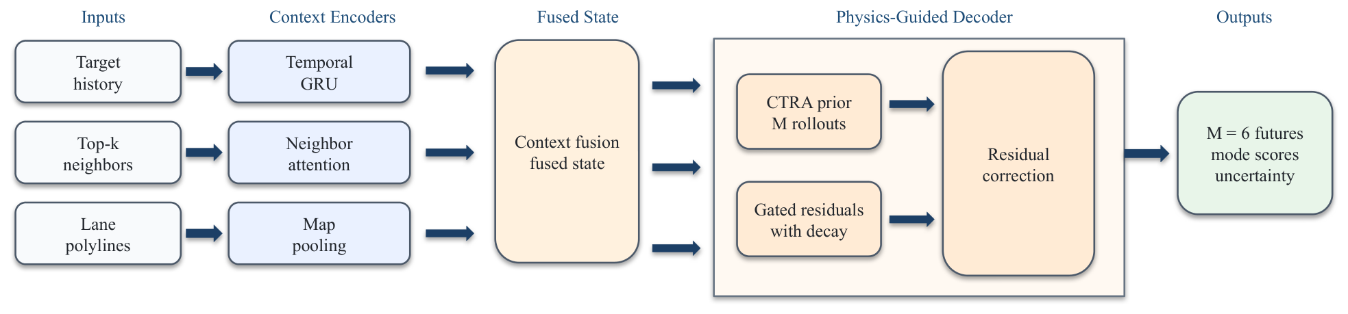
Architecture of the final compact CTRA–residual predictor. The model receives target history, four masked neighbor slots, and local lane polylines; the decoder rolls out six CTRA anchors, applies gated time-decayed autoregressive residual corrections, and outputs mode scores.
Figure 1.
Architecture of the final compact CTRA–residual predictor. The model receives target history, four masked neighbor slots, and local lane polylines; the decoder rolls out six CTRA anchors, applies gated time-decayed autoregressive residual corrections, and outputs mode scores.
Figure 2.
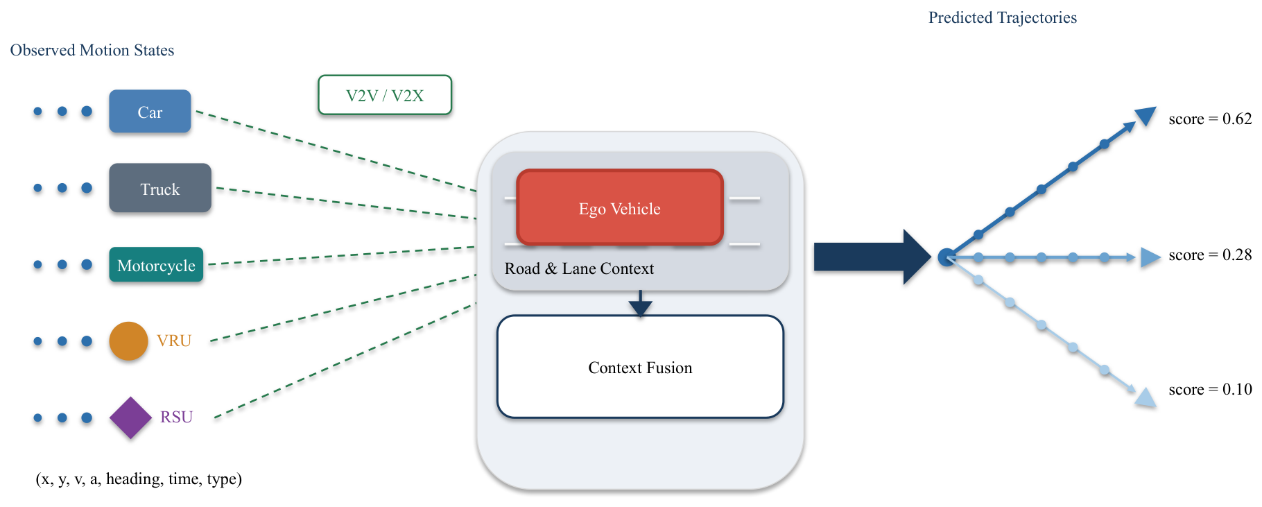
V2V/V2X-oriented forecasting interface used to explain the input scope. Colored blocks denote heterogeneous agent and context inputs, and arrows indicate the fusion path from observed states and road/lane context to ego-centered trajectory prediction. Observed motion states from heterogeneous agents and road/lane context are fused at the ego vehicle before the predictor outputs candidate trajectories with mode scores.
Figure 2.
V2V/V2X-oriented forecasting interface used to explain the input scope. Colored blocks denote heterogeneous agent and context inputs, and arrows indicate the fusion path from observed states and road/lane context to ego-centered trajectory prediction. Observed motion states from heterogeneous agents and road/lane context are fused at the ego vehicle before the predictor outputs candidate trajectories with mode scores.
Figure 3.
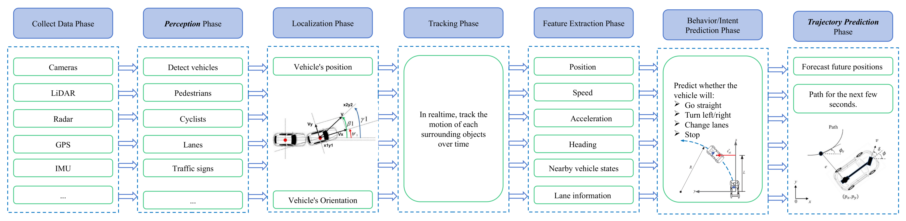
Data interface assumed in this study. Perception, localization, tracking, feature extraction, and behavior/intent estimation are treated as upstream stages; the trajectory predictor starts after target history, masked neighbor states, and lane context have already been converted into the target-centric frame. Ellipses denote omitted intermediate upstream processing steps and do not change the predictor inputs used in this study.
Figure 3.
Data interface assumed in this study. Perception, localization, tracking, feature extraction, and behavior/intent estimation are treated as upstream stages; the trajectory predictor starts after target history, masked neighbor states, and lane context have already been converted into the target-centric frame. Ellipses denote omitted intermediate upstream processing steps and do not change the predictor inputs used in this study.
Figure 4.
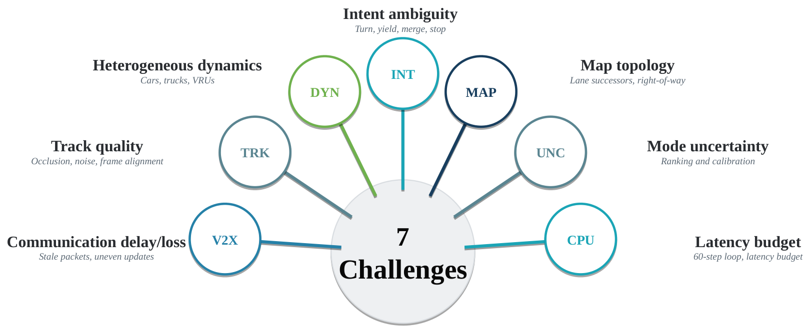
Seven trajectory-prediction challenges represented in the revised circular graphic: communication delay/loss, track quality, heterogeneous dynamics, intent ambiguity, map topology, mode uncertainty, and latency budget.
Figure 4.
Seven trajectory-prediction challenges represented in the revised circular graphic: communication delay/loss, track quality, heterogeneous dynamics, intent ambiguity, map topology, mode uncertainty, and latency budget.
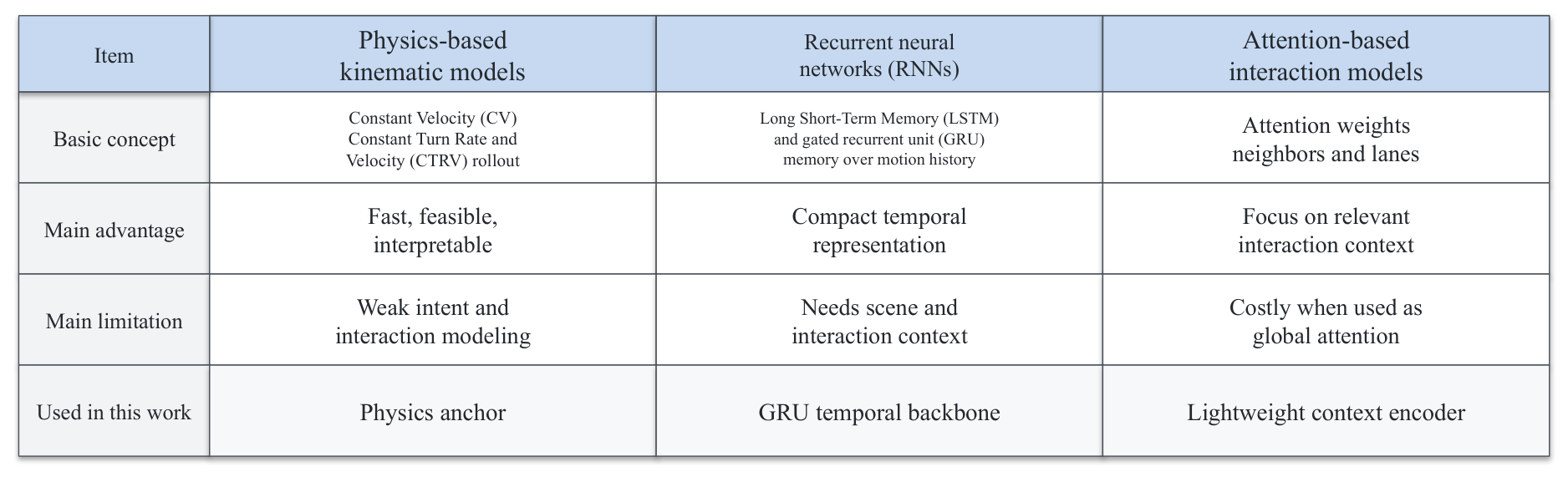
Figure 5.
Table-style comparison of the investigated algorithm families. The final model keeps the physics-based family as the rollout anchor, the recurrent family as the GRU temporal backbone, and the attention family as a lightweight context encoder.
Figure 5.
Table-style comparison of the investigated algorithm families. The final model keeps the physics-based family as the rollout anchor, the recurrent family as the GRU temporal backbone, and the attention family as a lightweight context encoder.
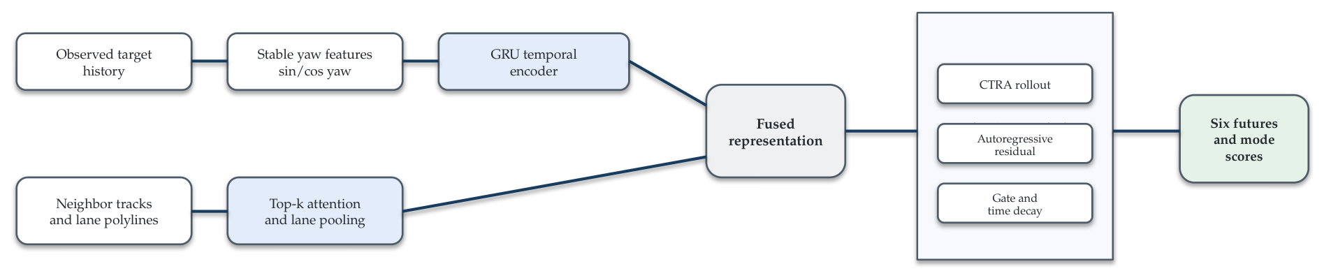
Figure 6.
Selected hybrid prediction pipeline after the sanity ablations. The upper branch encodes target history, the lower branch encodes neighbor/lane context, and the fused representation drives the CTRA-residual decoder.
Figure 6.
Selected hybrid prediction pipeline after the sanity ablations. The upper branch encodes target history, the lower branch encodes neighbor/lane context, and the fused representation drives the CTRA-residual decoder.
Figure 7.
Developed enhancements added beyond the investigated baseline families. These items are separated from the pipeline figure to distinguish architectural flow from implementation changes.
Figure 7.
Developed enhancements added beyond the investigated baseline families. These items are separated from the pipeline figure to distinguish architectural flow from implementation changes.
Figure 10.
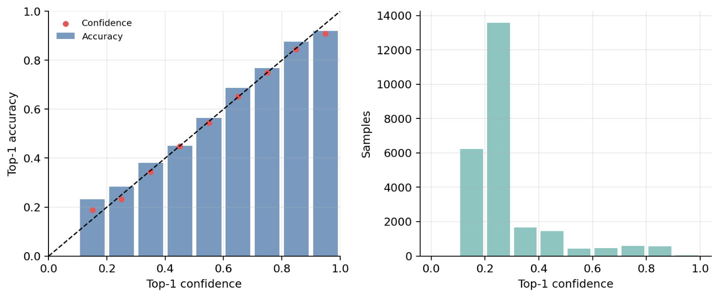
Calibration diagnostics for top-1 mode confidence on the validation export. (Left): reliability diagram, where the dashed line denotes perfect calibration. (Right): distribution of top-1 confidence values across validation samples.
Figure 10.
Calibration diagnostics for top-1 mode confidence on the validation export. (Left): reliability diagram, where the dashed line denotes perfect calibration. (Right): distribution of top-1 confidence values across validation samples.
Figure 11.
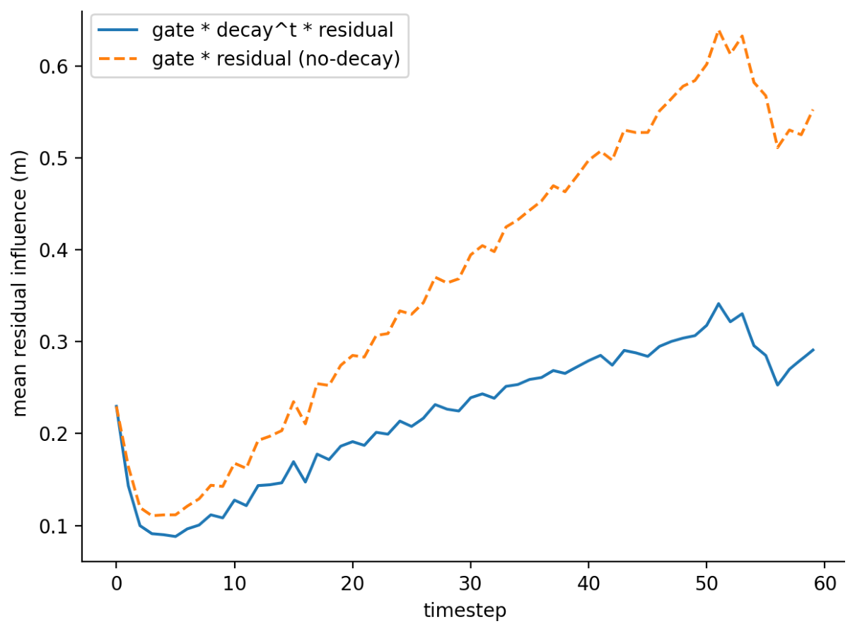
Mean residual influence magnitude vs. time, computed over 5120 validation instances and averaged over modes. The plotted residual influence is the product of gate, decay, and residual magnitude. Although residual magnitude tends to grow with horizon, learned decay damps its influence relative to a no-decay counterfactual derived from the same forward pass.
Figure 11.
Mean residual influence magnitude vs. time, computed over 5120 validation instances and averaged over modes. The plotted residual influence is the product of gate, decay, and residual magnitude. Although residual magnitude tends to grow with horizon, learned decay damps its influence relative to a no-decay counterfactual derived from the same forward pass.
Table 1.
Comparison of Representative Trajectory Prediction Approaches.
Table 1.
Comparison of Representative Trajectory Prediction Approaches.
| Method | Year | Temporal Encoder | Social Aware | Map Aware | Physics Prior | Multi-Modal |
|---|
| KF-CTRV [5] | 2022 | – | – | – | ✓ | – |
| IA-LSTM [12] | 2024 | LSTM | ✓ | – | – | – |
| IMA-LSTM [13] | 2024 | LSTM | ✓ | – | – | – |
| HeteroEdge-GAT [14] | 2022 | – | ✓ | ✓ | – | – |
| ST-GCN [15] | 2022 | – | ✓ | – | – | – |
| Dual-Branch GNN [16] | 2023 | – | ✓ | ✓ | – | – |
| Diffusion GCN [29] | 2024 | – | ✓ | – | – | ✓ |
| ST Graph Attention Transformer [18] | 2022 | Transformer | ✓ | (✓) | – | – |
| MTR [21] | 2022 | Transformer | ✓ | ✓ | – | ✓ |
| HDGT [19] | 2023 | Transformer | ✓ | ✓ | – | – |
| KA-MGAT [25] | 2024 | GAT | ✓ | – | ✓ | ✓ |
| HATN [20] | 2025 | Transformer | ✓ | ✓ | (✓) | ✓ |
| CVAE (Multi-task) [32] | 2025 | LSTM | ✓ | ✓ | – | ✓ |
| MTGNet [33] | 2025 | Transformer | ✓ | ✓ | – | ✓ |
| CVAE+Bicycle [23] | 2024 | LSTM | ✓ | ✓ | ✓ | ✓ |
| HRGC [26] | 2025 | Transformer | ✓ | ✓ | ✓ | ✓ |
| CMTT [22] | 2026 | Transformer | ✓ | ✓ | – | ✓ |
| This Work | 2026 | GRU | ✓ | ✓ | CTRA+Gate | ✓ |
Table 2.
Argoverse 2 Motion Forecasting split sizes (number of sequences).
Table 2.
Argoverse 2 Motion Forecasting split sizes (number of sequences).
| Split | Sequences |
|---|
| Training | 199,908 |
| Validation | 24,988 |
| Test | 24,984 |
Table 3.
Loss-weight, scoring, and residual-gate sensitivity on 10k/2k sanity runs. Rows are representative coarse validation runs, not a full grid search.
Table 3.
Loss-weight, scoring, and residual-gate sensitivity on 10k/2k sanity runs. Rows are representative coarse validation runs, not a full grid search.
| Variant | minADE6 | minFDE6 | Top1Acc | Top1Conf |
|---|
| Default weights, gate bias 1.0 | 1.861 | 4.306 | 0.328 | 0.324 |
| Gate bias 0.5 | 1.930 | 4.452 | 0.209 | 0.206 |
| Gate bias 0.0 | 1.905 | 4.387 | 0.366 | 0.329 |
| No physics gate | 2.121 | 4.946 | 0.270 | 0.267 |
| Waypoint/lane aux. () | 1.867 | 4.297 | 0.264 | 0.263 |
| Waypoint/lane aux. () | 1.866 | 4.304 | 0.347 | 0.299 |
| Soft assignment + calibration () | 2.139 | 5.745 | 0.239 | 0.174 |
| TTC/risk neighbor weight 1.0 | 1.974 | 4.490 | 0.277 | 0.249 |
Table 4.
Training hyperparameters.
Table 4.
Training hyperparameters.
| Parameter | Value | Parameter | Value |
|---|
| Optimizer | AdamW | Learning rate | |
| Weight decay | | Batch size | 1024 |
| Epochs | 65 | Gradient clipping | 5.0 |
| Scheduler | ReduceLROnPlateau | Patience (scheduler) | 3 epochs |
| Learning-rate decay factor | 0.5 | Minimum learning rate | |
| Dropout rate | 0.2 | Hidden dimension | 256 |
| Neighbor hidden dim | 128 | Map hidden dim | 128 |
| Correction GRU hidden | 128 | Correction GRU layers | 2 |
| Gate bias init | 1.0 | Number of modes | 6 |
| Neighbor radius | 30 m | Top-k neighbors | 4 |
Table 5.
Quantitative results on Argoverse 2 (). Argoverse 2 baseline rows are reported from the Argoverse 2 dataset paper; QCNet/ProphNet are high-capacity published references. Top1Acc/Top1Conf are reported for the proposed model to summarize mode ranking quality.
Table 5.
Quantitative results on Argoverse 2 (). Argoverse 2 baseline rows are reported from the Argoverse 2 dataset paper; QCNet/ProphNet are high-capacity published references. Top1Acc/Top1Conf are reported for the proposed model to summarize mode ranking quality.
| Method | Reference Group | minADE6 | minFDE6 | Top1Acc | Top1Conf |
|---|
| Argoverse 2 nearest-neighbor baseline [4] | Dataset baseline | 2.18 | 4.94 | – | – |
| Argoverse 2 WIMP baseline [4] | Dataset baseline | 1.47 | 2.90 | – | – |
| Proposed model | Compact physics-guided | 1.21 | 2.78 | 0.318 | 0.278 |
| QCNet [42] | High-capacity reference | 0.73 | 1.27 | – | – |
| ProphNet [43] | High-capacity reference | 0.68 | 1.33 | – | – |
Table 6.
Additional validation diagnostics for mode selection, diversity, and calibration.
Table 6.
Additional validation diagnostics for mode selection, diversity, and calibration.
| Metric | Value |
|---|
| ADE1/FDE1 | 3.12 m / 8.17 m |
| MR6 at 2 m | 48.2% |
| ECE | 0.044 |
| Mean endpoint spread | 15.57 m |
| Mean path spread | 5.74 m |
| Normalized mode entropy | 0.903 |
Table 7.
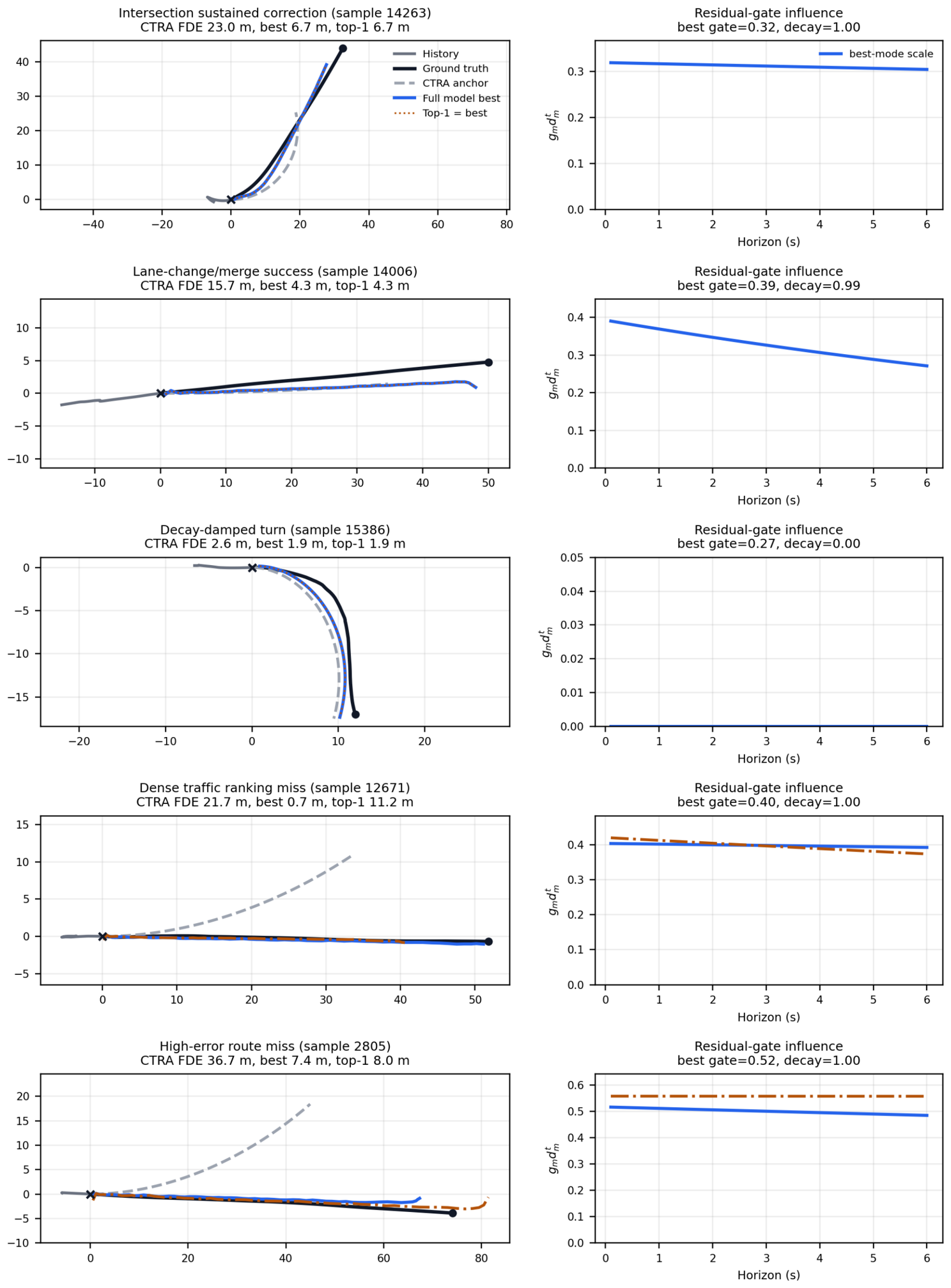
Concrete case-study metrics from
Figure 9. CTRA FDE is measured on the same mode that is oracle-best after residual correction.
Table 7.
Concrete case-study metrics from
Figure 9. CTRA FDE is measured on the same mode that is oracle-best after residual correction.
| Case | Neigh. | CTRA FDE | Full-Best FDE | Top-1 FDE | Gate/Decay |
|---|
| Intersection sustained correction | 0 | 23.0 | 6.7 | 6.7 | 0.32/0.999 |
| Lane-change/merge success | 4 | 15.7 | 4.3 | 4.3 | 0.39/0.994 |
| Decay-damped turn | 4 | 2.6 | 1.9 | 1.9 | 0.27/0.000 |
| Dense traffic ranking miss | 3 | 21.7 | 0.7 | 11.2 | 0.40/1.000 |
| High-error route miss | 4 | 36.7 | 7.4 | 8.0 | 0.52/0.999 |
Table 8.
Scenario-level diagnostic breakdown on the validation split. Scenario tags are heuristic and can overlap.
Table 8.
Scenario-level diagnostic breakdown on the validation split. Scenario tags are heuristic and can overlap.
| Scenario | n | minADE6 | minFDE6 | MR6 | Top1Acc |
|---|
| Lane following | 1083 | 0.87 | 1.81 | 31.6% | 0.299 |
| Intersection context | 22,396 | 1.24 | 2.85 | 49.0% | 0.329 |
| Turning | 5831 | 2.18 | 5.63 | 86.4% | 0.235 |
| Lane change/merge | 6284 | 2.13 | 5.43 | 86.1% | 0.221 |
| Dense neighbors (≥3) | 13,040 | 1.17 | 2.67 | 45.7% | 0.356 |
Table 9.
Post-hoc temperature scaling from saved validation probabilities. The split uses a deterministic 20% calibration subset and 80% evaluation subset.
Table 9.
Post-hoc temperature scaling from saved validation probabilities. The split uses a deterministic 20% calibration subset and 80% evaluation subset.
| Setting | Temperature | Top1Acc | Top1Conf | ECE |
|---|
| Uncalibrated | 1.00 | 0.324 | 0.282 | 0.043 |
| Temperature scaled | 0.80 | 0.324 | 0.303 | 0.038 |
Table 10.
Sanity ablations on a 10k/2k subset (). All runs use and the legacy decoder.
Table 10.
Sanity ablations on a 10k/2k subset (). All runs use and the legacy decoder.
| Variant | minADE6 | minFDE6 | Top1Acc | Top1Conf |
|---|
| CTRA-only (no residuals) | 2.939 | 7.189 | – | – |
| Non-autoregressive residuals (baseline) | 1.915 | 4.532 | 0.312 | 0.296 |
| Autoregressive residuals | 1.890 | 4.331 | 0.322 | 0.249 |
| Autoregressive + bigger GRU | 1.824 | 4.157 | 0.399 | 0.337 |
| Autoregressive + bigger GRU + gate bias 1.0 | 1.861 | 4.306 | 0.328 | 0.324 |
| Autoregressive + bigger GRU (no gate) | 2.121 | 4.946 | 0.270 | 0.267 |
| Control-space residuals | 2.468 | 6.159 | 0.298 | 0.300 |
Table 11.
Model size (final configuration).
Table 11.
Model size (final configuration).
| Metric | Value |
|---|
| Parameters | 1.78 M |
| Model size (FP32) | 6.8 MB |
Table 12.
Forward-pass latency of the proposed model on the development laptop. Central processing unit (CPU) results use an AMD Ryzen 7 7735HS; CUDA results use an NVIDIA GeForce RTX 4050 Laptop GPU.
Table 12.
Forward-pass latency of the proposed model on the development laptop. Central processing unit (CPU) results use an AMD Ryzen 7 7735HS; CUDA results use an NVIDIA GeForce RTX 4050 Laptop GPU.
| Device | Batch Size | ms/Sample | Samples/s |
|---|
| CPU | 1 | 82.7 | 12.1 |
| CPU | 32 | 3.5 | 286.6 |
| CUDA | 1 | 144.3 | 6.9 |
| CUDA | 32 | 4.8 | 206.4 |
| CUDA | 256 | 1.2 | 810.6 |
Table 13.
Published latency context for transformer-based references. These rows use different hardware and prediction protocols, so they are provided as context rather than a direct benchmark against
Table 12.
Table 13.
Published latency context for transformer-based references. These rows use different hardware and prediction protocols, so they are provided as context rather than a direct benchmark against
Table 12.
| Method | Hardware | Published Latency Protocol |
|---|
| Proposed model | Ryzen 7 7735HS / RTX 4050 laptop | This work: focal-agent forward pass; 82.7 ms at CPU batch 1, 3.5 ms/sample at CPU batch 32, and 1.2 ms/sample at CUDA batch 256. |
| QCNet [42] | NVIDIA A40 | The QCNet supplementary material reports 46 ms for predicting all agents in an average Argoverse 2 scene and 72 ms for a dense scene with 190 agents. |
| ProphNet [43] | NVIDIA V100 | Published latency analysis reports 28.0 ms and 0.40 GFLOPs with 64 agents. |
Table 14.
Negative results on sanity runs (10k/2k, ). The effect column summarizes the observed failure mode.
Table 14.
Negative results on sanity runs (10k/2k, ). The effect column summarizes the observed failure mode.
| Variant | minADE6 | minFDE6 | Observed Effect |
|---|
| Goal conditioning | 1.953 | 4.623 | Wrong lane goals propagate through residual rollout. |
| Map cross-attention | 2.100 | 4.791 | More local geometry, but no lane connectivity or route state. |
| Soft assignment + calibration | 2.139 | 5.745 | Weaker winner signal; confidence collapses to 0.174 Top1Conf. |
| TTC/risk neighbor weight | 1.974 | 4.490 | Local risk cue does not resolve route intent. |
| Control-space residuals | 2.468 | 6.159 | Small control errors integrate into large endpoint drift. |
| Multi-head decoder | 2.220 | 5.161 | Per-head supervision is fragmented in the compact subset. |




 ,
,