Automatic Detection of TiO₂ Nanoparticles Using Dual-Coupled Microresonators and Deep Learning

Abstract

The detection of titanium dioxide (${\mathrm{TiO}}_2$) nanoparticles is a significant challenge due to their extensive industrial use and potential health and environmental impacts, which demand accurate, label-free approaches. This work presents an automatic detection system based on spectroscopy with optical frequency combs (OFC) in dual-coupled microresonators. The OFC generation was modeled through the Lugiato-Lefever equation, while propagation in distilled water containing ${\mathrm{TiO}}_2$ was simulated using the finite element method (FEM). The water–${TiO}_2$ mixture was described with the Yamaguchi model in a 5 × 5 mesh to represent non-uniform concentrations. From the norm of the electric field at a probe, a database of 11 classes (0–100%) with controlled Gaussian noise was constructed. A Transformer-based classifier was trained and compared with 1D-CNN and SVM under Monte Carlo validation (100 random 70/30 splits). The Transformer achieved 99.84 ± 0.01% accuracy with an inference time of 0.793 ± 0.05 s, while the 1D-CNN reached 99.64 ± 0.09% and the SVM 84.73 ± 1.48%. A repeatability test with 200 iterations confirmed deterministic DKS trajectories. The results demonstrate that combining dual-coupled microresonators, FEM, and Transformer architectures enables precise and efficient detection of ${\mathrm{TiO}}_2$ nanoparticles in aqueous solutions.

1. Introduction

Titanium dioxide (${\mathrm{TiO}}_2$) nanoparticles (NPs) are extensively utilized in pharmaceutical, cosmetic, food, and environmental applications owing to their outstanding optical, photocatalytic, and chemical properties [1,2,3]. However, their widespread deployment has raised increasing concerns regarding potential adverse effects on human health and aquatic ecosystems. These concerns underscore the need for sensitive, label-free, and real-time techniques capable of accurately detecting and quantifying nanoparticles. In this context, optical spectroscopy emerges as a powerful, non-invasive, and high-resolution tool for probing light–matter interactions in complex media.

Several optical spectroscopic techniques have been widely explored for nanoparticle detection, notably Raman spectroscopy and surface-enhanced Raman scattering (SERS). Raman-based methods provide molecular-specific vibrational fingerprints and enable label-free identification of chemical composition in complex media [4,5]. SERS further enhances detection sensitivity by exploiting localized plasmonic field amplification, enabling trace-level analysis in aqueous environments [6,7]. Despite their high sensitivity, these approaches often rely on complex substrate preparation, plasmonic nano-structures, or exhibit limited reproducibility and limited spectral bandwidth, which constrain their scalability for broadband and real-time sensing applications. These limitations have motivated the development of alternative broadband and highly coherent optical spectroscopy techniques.

Within this context, optical frequency combs (OFCs) have emerged as highly effective light sources for broadband spectroscopy. Their discrete, equally spaced, and phase-coherent spectral lines provide uniform frequency coverage across wide bandwidths, enabling precise measurements of absorption features, refractive index variations, and scattering phenomena [8,9]. Consequently, OFCs have proven to be powerful tools for biosensing and nanoparticle detection in aqueous environments. In the time domain, an OFC can be interpreted as a train of ultrashort pulses whose Fourier transform yields the comb-like structure in the frequency domain.

Depending on the operating conditions, various nonlinear regimes can be sustained in microresonators, including Turing rolls, cnoidal waves, and dissipative Kerr solitons (DKS) [8]. Although OFCs were originally developed for precision metrology and optical communications [8,9,10], their extension to sensing has opened new frontiers in high-resolution spectroscopy, enabling label-free nanoparticle characterization [11]. Common generation techniques include four-wave mixing (FWM) in microresonators, electro-optic modulation, and mode-locked lasers [9]. However, these systems often face challenges such as limited spectral stability, low conversion efficiency, and stringent tuning requirements, motivating the exploration of alternative, more scalable schemes.

Microring resonators (MRRs) have long been recognized as compact and highly sensitive photonic platforms for nanoparticle sensing. Their high quality factors and strong light confinement enable detection of resonance wavelength shifts induced by changes in the effective refractive index through particle–evanescent field interactions [11,12,13,14]. Such mechanisms allow quantitative estimation of particle size, composition, and concentration in aqueous media. Nonetheless, traditional MRR sensors rely on single-resonance interrogation, limiting their spectral information and sensitivity.

Dissipative Kerr solitons (DKS) generated in optical microresonators provide a broadband, phase-coherent solution to this limitation. The delicate balance between Kerr nonlinearity and group-velocity dispersion leads to the formation of temporally localized pulses whose frequency-domain representation consists of hundreds of evenly spaced lines [15]. This dense, coherent structure significantly enhances signal-to-noise ratio and spectral sensitivity, enabling label-free sensing over multiple wavelength channels. Despite their advantages, DKS generation remains experimentally demanding. The soliton existence region in the detuning–pump parameter space is typically narrow, and system trajectories often traverse chaotic regimes that destabilize soliton formation. Strategies such as dispersion engineering, optical feedback, and thermal control have been implemented to address these issues, though they often increase system complexity or reduce fabrication tolerance [16,17,18,19].

Dual-coupled microring resonators (DCMs) have recently emerged as an attractive platform for overcoming these limitations. By introducing a secondary coupling pathway, DCMs enable precise control over avoided mode crossings, which constitute one of the primary sources of instability in single-ring systems. Properly engineered inter-ring coupling can suppress parasitic modal interactions and expand the stability window for soliton formation, enabling deterministic and reproducible DKS generation. This architecture thus offers enhanced robustness to fabrication variations and improved spectral tunability, paving the way for practical DKS-based frequency comb spectroscopy in nanoparticle detection [20,21,22,23,24].

Despite the growing maturity of DKS-based comb generation, most reported sensing studies and machine learning integrations remain confined to single-resonance microresonator sensors or conventional broadband spectroscopy, where the full information encoded in DKS combs is underutilized. Consequently, the potential of frequency-comb spectroscopy for fully automatic nanoparticle detection remains largely unexplored.

Classical machine learning algorithms such as support vector machines (SVM), principal component analysis (PCA), Gaussian processes (GP), and clustering techniques have been successfully applied to spectral data from scattering and Raman measurements [2,3,4,7,25]. However, these approaches rely on handcrafted feature extraction and exhibit limited robustness in noisy or nonlinear regimes. The advent of deep learning has mitigated these limitations: Convolutional Neural Networks (CNNs) have demonstrated remarkable accuracy in Raman and infrared spectroscopy by autonomously learning hierarchical spectral features [5,6,26,27,28]. Recurrent models such as Long Short-Term Memory (LSTM) networks and autoencoders have further enabled time-resolved optical analysis. Nevertheless, their capacity to model long-range dependencies remains limited.

Transformer architectures have recently redefined spectral analysis through their self-attention mechanism, which effectively captures both local and global relationships in complex signals. Although their use in optical spectroscopy and nanoparticle sensing is still emerging, initial studies suggest that Transformers are particularly suited for analyzing rich, multi-component spectra such as those produced by DKS combs. This convergence of frequency-comb spectroscopy and advanced deep learning represents a promising direction: OFC-based systems offer unparalleled spectral resolution and phase coherence, while models like CNNs and Transformers can exploit such information for fully automatic, label-free, and highly accurate nanoparticle detection.

This work introduces an integrated framework combining deterministic DKS generation in dual-coupled microring resonators, optical field propagation modeling using the finite element method (FEM) coupled with the Yamaguchi scattering model, and deep learning architectures, particularly Transformers for the automatic detection of ${\mathrm{TiO}}_2$ nanoparticles. The integration of dual-coupled microring-based DKS spectroscopy with Transformer-based learning for nanoparticle detection has not been explicitly addressed in prior studies. The proposed methodology aims to overcome the limitations of conventional narrowband and manually engineered approaches, enabling robust, data-driven classification of ${\mathrm{TiO}}_2$ concentrations in aqueous media. This integration of photonic modeling and artificial intelligence establishes a foundation for next-generation sensing systems with potential applications in biomedical diagnostics, chemical analysis, and environmental monitoring.

2. Materials and Methods

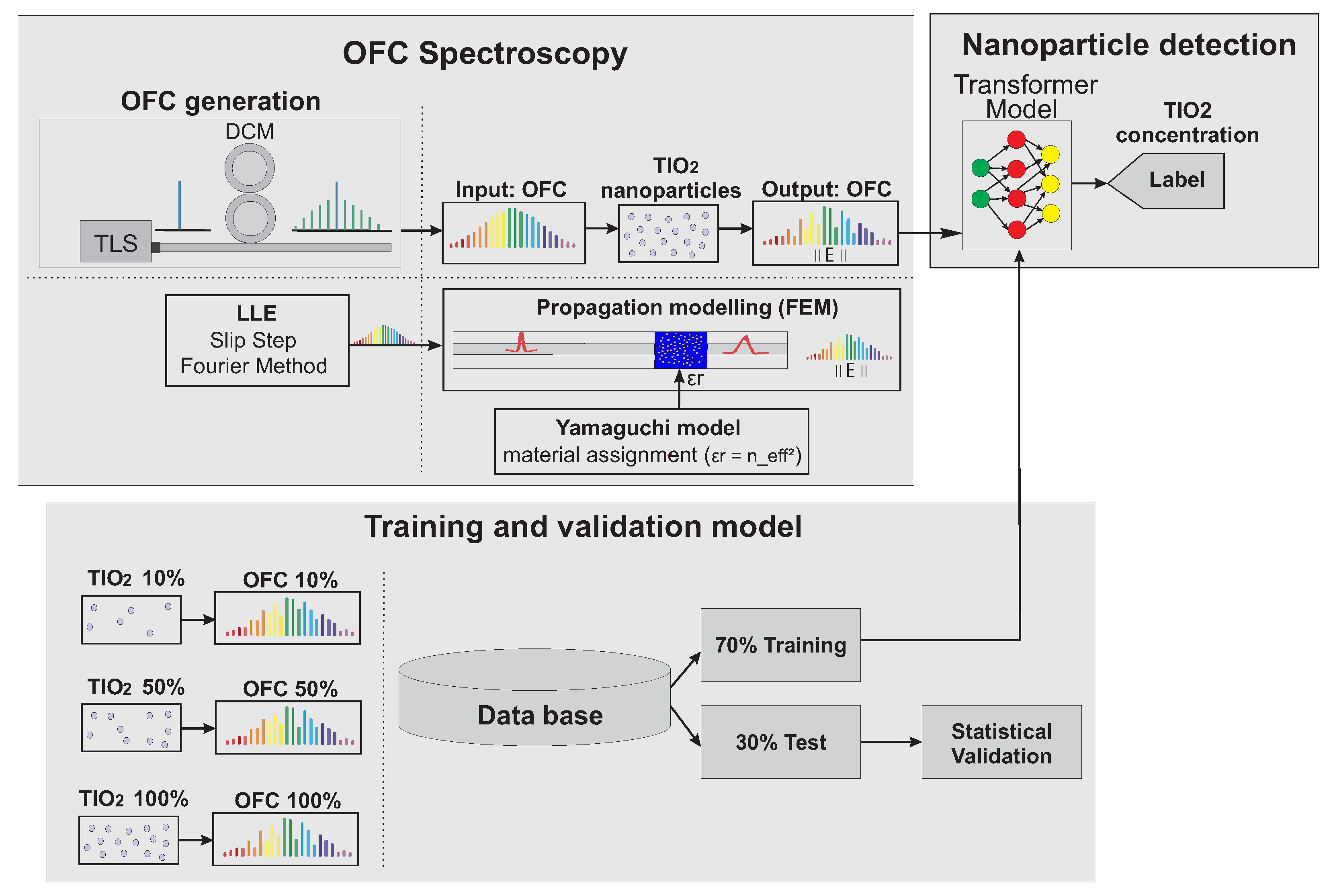
This study proposes an automated framework for ${\mathrm{TiO}}_2$ nanoparticle detection that integrates dual-coupled microring (DCM) frequency-comb spectroscopy with physics-driven simulations and supervised machine learning. In this approach, DKS generated in DCM serve as a broadband, phase-coherent optical source, enabling spectrally rich excitation across multiple wavelength channels. Synthetic datasets derived from full-wave FEM simulations model light propagation in ${\mathrm{TiO}}_2$ suspensions. A Transformer architecture specifically adapted to one-dimensional signals is implemented for classification, and the results are validated against architectures and methods commonly reported in the literature. The framework is validated through Monte Carlo cross-validation to ensure robust and unbiased performance, as summarized in Figure 1.

2.1. DKS Generation in Dual-Coupled Microrings

To obtain the optical excitation used throughout this study, we employ a dual-coupled microring (DCM) configuration to generate DKS pulses, modeled by the Lugiato–Lefever equation (LLE) with intermodal coupling. The choice of DCM stems from its modal-engineering flexibility: by manipulating avoided mode crossings (AMX), the DCM enables precise dispersion control and expands the operational window for deterministic and stable DKS generation. The LLE governing the intracavity field is:

$${\displaystyle \frac{\partial \psi }{\partial T}}=-i\left[{\displaystyle \frac{8{\pi }^{3}R}{t_R^2}}{\displaystyle \frac{{\beta }_2}{2\alpha }}\right]{\displaystyle \frac{{\partial }^2\psi }{\partial {\theta }^2}}+i{\left|\psi \right|}^2\psi -(i\mathsf{\Delta }+1)\psi +S+i{\displaystyle \frac{1}{\alpha }}\sum _{\mu }\left[{\displaystyle \frac{a/2}{\mu -b}}{\tilde{\psi }}_{\mu }\left(T\right)e^{i\mu \theta }\right]$$

(1)

with spectral components

$${\tilde{\psi }}_{\mu }\left(T\right)={\displaystyle \frac{1}{2\pi }}{\mathit{\int }}_0^{2\pi }\psi (T, \theta )e^{-i\mu \theta }d\theta$$

(2)

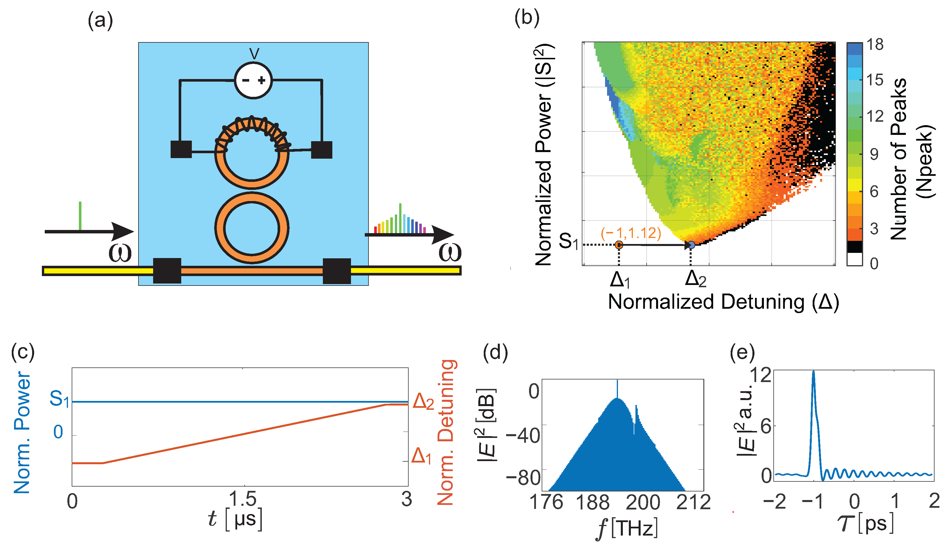
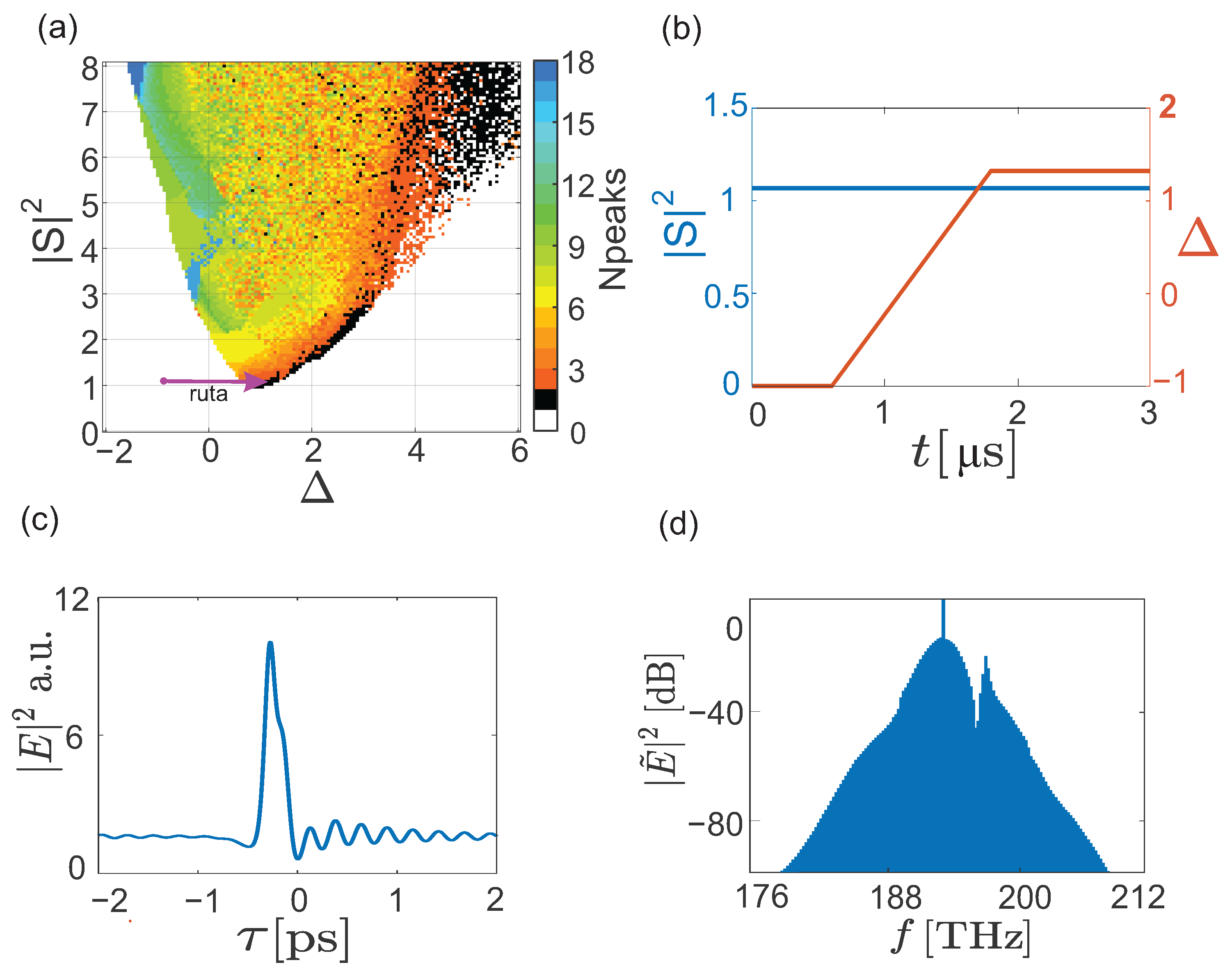
In Equation (1), the pump term S and the detuning parameter $\mathsf{\Delta }$ define the operating regime of the microresonator and control the transition from modulation instability to stable DKS states. The group-velocity dispersion coefficient ${\beta }_2$ governs the DKS temporal width and, consequently, the spectral bandwidth of the generated optical frequency comb. Cavity losses ($\alpha$) account for attenuation in the resonator and influence the accessible operating window and stability of the DKS states. In the DCM configuration, the avoided mode crossings, parameterized by a and b, provide additional dispersion engineering and expand the accessible DKS existence region. Numerical integration is performed with a split-step Fourier method. The dual-coupled microring (DCM) parameters are set to the values reported in [29]: principal radius $R=100\mathrm{\mu }$m, $t_R=1/226$ GHz, ${\beta }_2=-4.7\times {10}^{-26}{\mathrm{ s}}^2$/m, $\alpha =1.61\times {10}^{-3}$, $\gamma =1.09 {\mathrm{W}}^{-1}{\mathrm{m}}^{-1}$, $L=2\pi \times 100\mathrm{\mu }$m, and $\theta =6.4\times {10}^{-4}$. We set $a=2\pi \times 9.71$ GHz and $b=13.44$ to shift the DKS region as observed in simulation. The pump for the single MRR case starts at detuning $\mathsf{\Delta }=0$ with input power ${\left|P_{\mathrm{in}}\right|}^2=5$ (47.6 mW) to ensure a stable comb at initialization. Following the approach described in [29], the path for DKS generation is established by configuring the LLE-based simulation to explore the parametric space $(\mathsf{\Delta }, {\left|S\right|}^2)$. The initial field $E\left(\omega \right)$ is defined as complex Gaussian noise with a standard deviation of ${\sigma }_{\mathrm{noise}}={10}^{-9}$ [${\mathrm{W}}^{1/2}$]. The system remains at the initial state $({\mathsf{\Delta }}_1, {\left|S_1\right|}^2)$ for $1.5\mathrm{\mu }$s, then transitions to $({\mathsf{\Delta }}_2, {\left|S_2\right|}^2)$, where it remains for the same interval. This process is repeated across the endpoints to reconstruct the parameter map. From this map, we select a path defined by constant pump power ${\left|S\right|}^2$ and a linearly varying detuning $\mathsf{\Delta }$, corresponding to a swept-laser scheme that enables access to the DKS region (lower-right area of the map). This controlled trajectory avoids the chaotic modulation-instability zone and promotes stable DKS generation. The graphical representation of this procedure is presented in Figure 2.

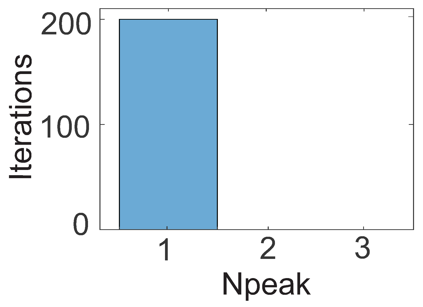
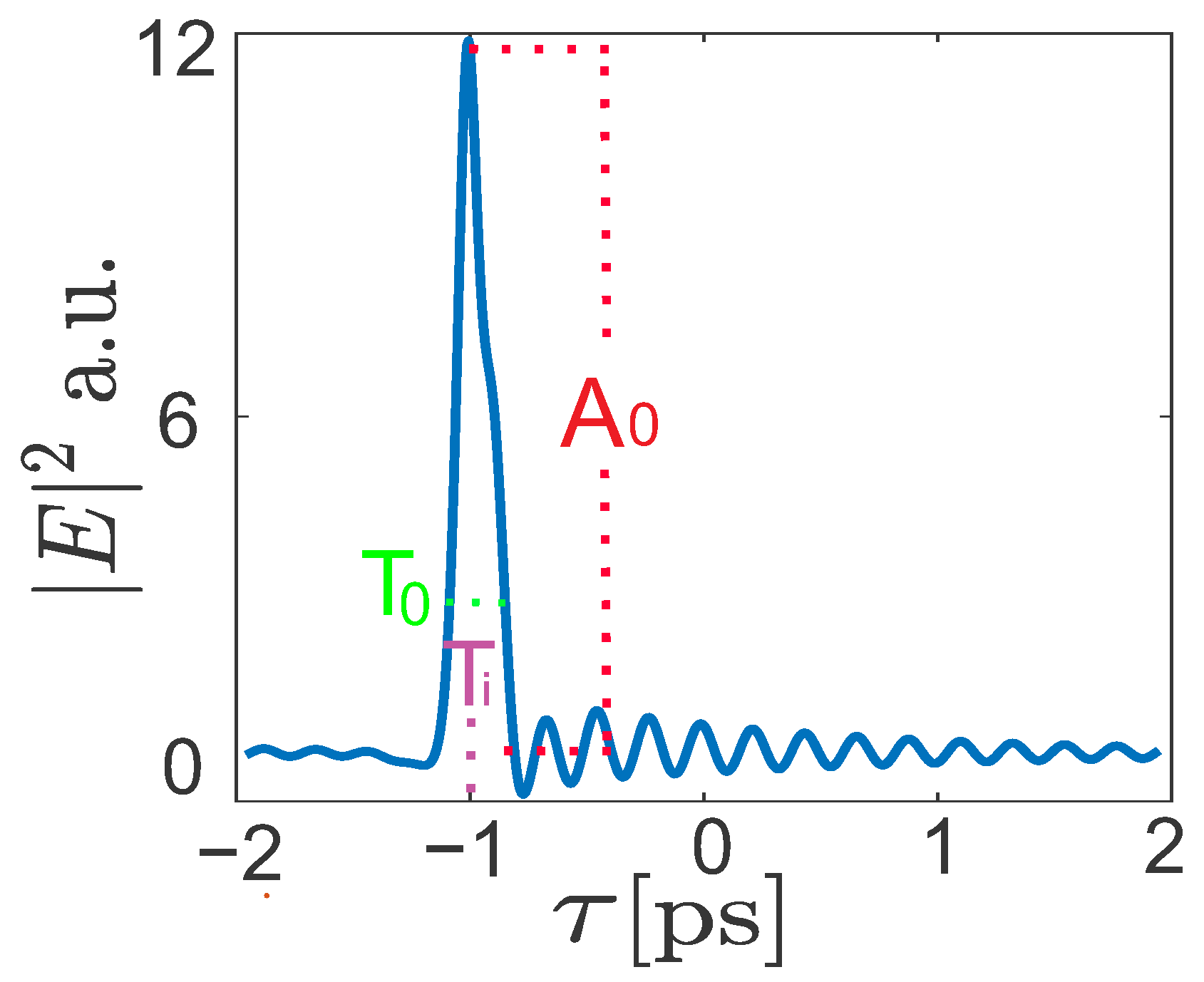
To ensure a reliable generation process, it is essential to assess whether DKS generation is deterministic. Determinism is evaluated by performing multiple numerical realizations of the LLE along a prescribed path. In each realization, the system is initialized with complex Gaussian noise and subsequently evolved under constant pump power while the laser detuning is linearly swept. The process is deemed deterministic if a single soliton pulse consistently emerges at the end of each simulation, thereby indicating stable and reproducible DKS generation. This verification is conducted over 200 independent realizations, from which the probability of soliton-state occurrence is estimated. The frequency of each outcome is quantified and represented as a histogram, providing a statistical measure of the repeatability of the generation process [29]. Once the deterministic behavior is confirmed, the temporal characteristics of the DKS are quantitatively analyzed to ensure a physically consistent excitation for the propagation stage. The stabilized waveform is fitted to a hyperbolic secant envelope to extract the soliton’s amplitude $A_0$, temporal width $T_0$, and center position $t_i$. These parameters fully describe the pulse in the time domain while implicitly preserving its spectral properties through Fourier duality (See Figure 3), thus requiring fewer parameters to maintain coherence and energy equivalence. The resulting analytical $\mathrm{sech}$-shaped function serves as the excitation field in the FEM model, providing a realistic temporal boundary condition that enables accurate simulation of optical propagation through the ${\mathrm{TiO}}_2$-loaded waveguide. This temporal-to-spatial linkage ensures that the FEM stage reproduces the same solitonic behavior observed in the LLE framework, maintaining physical consistency between the generation and propagation models.

2.2. Database Construction (FEM Propagation and Yamaguchi Modeling)

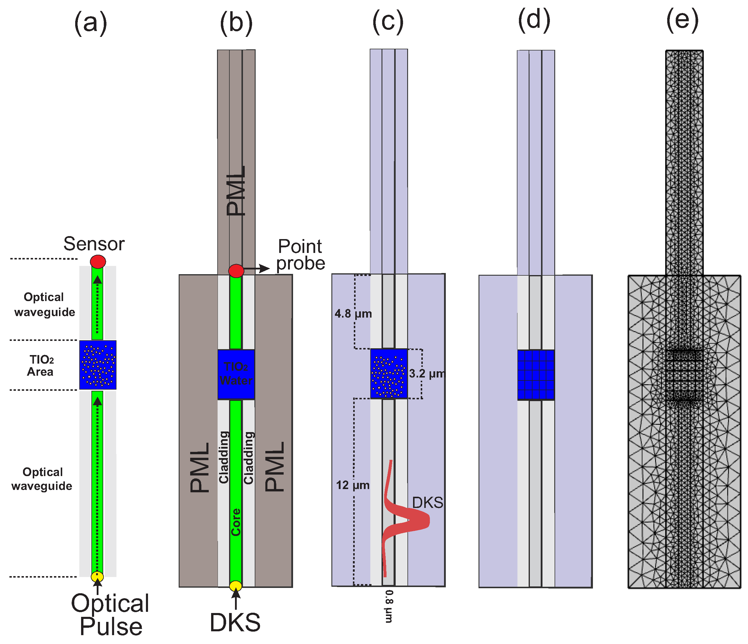
To construct the annotated database, we simulate the propagation of the previously characterized DKS excitation through distilled water containing ${\mathrm{TiO}}_2$ nanoparticles at different concentration levels. Each simulation represents a distinct physical scenario used to model the optical interaction between the DKS and the scattering medium. We record the electric field with a probe at the collector-waveguide output, producing time-resolved traces of its evolution throughout the simulation. Instead of monochromatic or line-by-line treatments, we compute propagation directly in the time domain, capturing the coupled evolution of all spectral components. The FEM model explicitly solves Maxwell’s equations in a two-dimensional $(x, y)$ cross-section under z-invariance, ensuring an accurate description of the field distribution and energy exchange mechanisms within the medium. The FEM model explicitly integrates Maxwell’s equations in a 2D $(x, y)$ domain, with invariance along z:

$${ϵ}_0{ϵ}_r(x, y){\displaystyle \frac{\partial \mathbf{E}(x, y, t)}{\partial t}}-\nabla \times \mathbf{H}(x, y, t)+\sigma (x, y)\mathbf{E}(x, y, t)=0$$

(3)

$${\mu }_0{\mu }_r(x, y){\displaystyle \frac{\partial \mathbf{H}(x, y, t)}{\partial t}}+\nabla \times \mathbf{E}(x, y, t)=0$$

(4)

with ${\epsilon }_r=n^2$ (Si₃N₄ core, ${\mathrm{SiO}}_2$ cladding, water $n=1.317$, ${\mathrm{TiO}}_{2}n=2.41$) and ${\mu }_r=1$. Perfectly Matched Layers (PMLs) are placed at the boundaries; the probe sits immediately before the output PML to avoid spurious reflections. The domain contains an input waveguide carrying the DKS, an interaction window (distilled water with ${\mathrm{TiO}}_2$ nanoparticles), and a collector waveguide. The measured observable is the electric-field magnitude

$$\parallel E\parallel =\sqrt{E_x^2+E_y^2},$$

which is proportional to the detected optical power.

An adaptive triangular mesh refines to element size $\le {\lambda }_0/5$ in the Si₃N₄ core for ${\lambda }_0=1.55\mathrm{\mu }$m, and gradually coarsens toward cladding and PML to reduce computational load. Material assignment follows the refractive-index models reported by [30] for ${\mathrm{SiO}}_2$ and by [31] for Si₃N₄, together with the relationships ${\epsilon }_r=n^2$ and ${\mu }_r=1$. The output probe registers E after interaction with the nanoparticle region, while the trailing PML prevents back-reflections into the measurement.

2.2.1. Analytical DKS Excitation for FEM

The input field at the waveguide is a temporal DKS contour derived from the LLE stage and parameterized as

$$f\left(t\right)=A_0·\mathrm{sech}\left({\displaystyle \frac{t-t_i}{T_0}}\right)$$

(5)

where $A_0$ is the amplitude, $T_0$ the width, and $t_i$ the time position of the soliton. These parameters are systematically varied within LLE-consistent ranges to reflect realistic variability in DKS generation.

2.2.2. Nanoparticle Distribution via Yamaguchi Effective Index

To simulate the optical behavior of the ${\mathrm{TiO}}_2$ nanoparticles suspended in water, we use the Yamaguchi effective-index model [19]. This model provides a macroscopic description of how a composite medium, consisting of a dielectric host with dispersed inclusions, modifies its effective refractive properties as a function of nanoparticle concentration. Rather than explicitly modeling individual nanoparticles, which would be computationally prohibitive due to their nanoscale dimensions and high number density, the Yamaguchi formulation establishes a relationship between the local particle volume fraction and the resulting effective permittivity of the mixture. The effective permittivity is expressed as

$${ϵ}_{\mathrm{ef}}={ϵ}_0\left(1+f{\displaystyle \frac{2({ϵ}_n-{ϵ}_0)}{{ϵ}_n+{ϵ}_0+f({ϵ}_n-{ϵ}_0)}}\right),n_{\mathrm{ef}}=\sqrt{{ϵ}_{\mathrm{ef}}},$$

(6)

where ${ϵ}_0$ and ${ϵ}_n$ are the permittivities of distilled water and ${\mathrm{TiO}}_2$, respectively, and $f={\displaystyle \frac{N\pi r^2}{WL}}$ denotes the nanoparticle area fraction within a region of dimensions $W\times L$.

This formulation enables the calculation of an effective refractive index $n_{\mathrm{ef}}$ that captures the collective dielectric response of the nanoparticle ensemble, effectively modeling the modification of the optical field as it propagates through the heterogeneous medium. To reproduce spatially varying concentrations, the interaction region is subdivided into a $5\times 5$ grid (Figure 4d).

The Yamaguchi model is used as an effective-medium approximation to represent the ${\mathrm{TiO}}_2$–water mixture through locally varying refractive-index values. By discretizing the interaction region into multiple sub-regions, the model introduces simplified spatial heterogeneity while remaining computationally efficient. Although nanoparticle-scale clustering and particle-resolved scattering are not explicitly modeled, this representation is sufficient for capturing concentration-dependent effects in the transient optical response relevant to the proposed sensing framework. Each cell represents a localized subregion of the domain to which a specific ${\mathrm{TiO}}_2$ concentration and corresponding effective refractive index are assigned. This discretization is necessary because the nanoparticle distribution in solution is inherently nonuniform. By dividing the medium into smaller cells, the simulation can emulate realistic spatial fluctuations in particle density and refractive properties, avoiding the oversimplification of treating the mixture as homogeneous. The $5\times 5$ configuration was chosen as a compromise between physical realism and computational efficiency, capturing fine-scale refractive variations without excessive numerical cost. The algorithm described in Algorithm 1 computes $n_{\mathrm{ef}}$ for each cell individually and then determines the overall effective index of the interaction area as the weighted average of all 25 cells. This approach enables the FEM model to incorporate both global and local variations in the optical response. From the cell-wise outputs, we compute an area-average effective index for labeling. Each FEM run yields the field at the probe; we report the optical signal via $\parallel E\parallel$, which correlates with detected optical power and captures interaction-induced changes.

Algorithm 1 Computing the effective refractive index using the Yamaguchi model
1: Stage 1: Per-cell calculations
2: Input:
3: $n_0\leftarrow 1.317$	▹ Base-medium refractive index (water)
4: $n_n\leftarrow 2.41$	▹ ${\mathrm{TiO}}_2$ nanoparticle refractive index.
5: $r\leftarrow 5\times {10}^{-9}$	▹ Radius of the nanoparticles [m]
6: $h\leftarrow 10\times {10}^{-9}$	▹ Height of the nanoparticles [m]
7: $W\leftarrow 0.8\times {10}^{-6}$	▹ Cell-area width [m]
8: $L\leftarrow 8\times W$	▹ Cell-area length [m]
9: $s\leftarrow 2\times {10}^{-9}$	▹ Nanoparticle edge-to-edge spacing [m]
10: $N\leftarrow 60$	▹ NUser-specified total number of nanoparticles
11: Initial calculations:
12: $d_{centros}\leftarrow 2r+s$	▹ Distance between nanoparticle centers
13: $A_n\leftarrow \pi r^2$	▹ Nanoparticle area
14: $N_{max\_fila}\leftarrow \lfloor W/d_{centros}\rfloor$	▹ Maximum nanoparticles per row (cell)
15: $N_{max\_columna}\leftarrow \lfloor L/d_{centros}\rfloor$	▹ Maximum nanoparticles per column (cell)
16: $max\_N\leftarrow N_{max\_fila}\times N_{max\_columna}$	▹ Total number of nanoparticles
17: $A_{n1}\leftarrow (W/N_{max\_fila})(L/N_{max\_columna})$	▹ Geometric area occupied by the nanoparticles
18: if $N>max\_N$ then
19:     Error: The number of nanoparticles exceeds the capacity of the specified area.
20: else
21:     $A_{total}\leftarrow W\times L$	▹ Total cell area
22:     $f\leftarrow (N\times A_n)/A_{total}$	▹ Fraction of area occupied by nanoparticles
23:     $f_O\leftarrow (N\times A_{n1})/A_{total}$	▹ Adjusted fraction
24:     ${ϵ}_0\leftarrow n_0^2$	▹ Permittivity of the base medium
25:     ${ϵ}_n\leftarrow n_n^2$	▹ Permittivity of the nanoparticle material
26:     ${ϵ}_{ef}\leftarrow {ϵ}_0\left(1+f{\displaystyle \frac{2({ϵ}_n-{ϵ}_0)}{{ϵ}_n+{ϵ}_0+f({ϵ}_n-{ϵ}_0)}}\right)$	▹ Effective permittivity.
27:     $n_{ef}\leftarrow \sqrt{{ϵ}_{ef}}$	▹ Effective refractive index
28:     Display results for the cell:
29:     Display Area fraction occupied and Nanoparticles number: $f_O$, N
30:     Display Maximum number of nanoparticles: $max\_N$
31:     Display Effective index of refraction and refractive index: $n_{ef}$, ${ϵ}_{ef}$
32: Stage 2: Computing the weighted average across all cells.
33: Input: $f_O$ values for the 25 cells
34: $\mathrm{percentage}\leftarrow {\sum }_{i=1}^{25}0.04\times f_O$	▹ Weighted mean of the 25 cells.

2.2.3. Signal Set and Class Labels

We generate an annotated dataset by varying ${\mathrm{TiO}}_2$ concentrations across the $5\times 5$ grid (nonuniform assignments per cell), producing 11 classes (0–100%) with 1000 samples per class (11,000 total). Each raw trace has 26,528 samples and is decimated by 15 to 1769 points to reduce computational cost while preserving salient structure. Zero-mean Gaussian noise with an amplitude of up to 10% of the signal is added to emulate generic sensor-level variability. More detailed noise sources, such as thermal or detector-specific contributions, are not explicitly modeled, as their inclusion would require instrument-dependent parameters beyond the scope of this study. The class distribution is reported in

Table 1. ${\mathrm{TiO}}_2$ database.

Class	Quantity	Class	Quantity
0%	1000	60%	1000
10%	1000	70%	1000
20%	1000	80%	1000
30%	1000	90%	1000
40%	1000	100%	1000
50%	1000

.

2.3. Automatic Detection Model (Transformer)

We formulate ${\mathrm{TiO}}_2$ concentration recognition from the temporal traces $\parallel E\parallel$ as a supervised multi-class problem and adopt a Transformer architecture tailored to one-dimensional signals. Each sample is a fixed-length sequence with 1769 points,

$${\mathbf{z}}_0=\mathbf{x}\in {\mathbb{R}}^{1769},$$

which we standardize to zero mean and unit variance. A sequenceInputLayer ingests $\mathbf{x}$ directly—positional encodings are not required because the temporal ordering is implicit. A flattenLayer preserves the vector structure for subsequent dense processing.

The first dense block maps the input to 512 latent units,

$${\mathbf{h}}_1={\mathbf{W}}_1\mathbf{x}+{\mathbf{b}}_1,{\mathbf{z}}_1=\mathrm{ReLU}\left({\mathbf{h}}_1\right),$$

followed by dropout with probability $p=0.23$ to reduce overfitting. We then apply a multi-head self-attention block with 8 heads, each operating in a 16-dimensional subspace; its concatenated output is linearly projected and layer-normalized:

$${\mathbf{z}}_2=\mathrm{Concat}({\mathrm{head}}_1, \dots , {\mathrm{head}}_8){\mathbf{W}}^O,{\mathbf{z}}_2^{\mathrm{norm}}=\mathrm{LayerNorm}\left({\mathbf{z}}_2\right).$$

A second dense transformation with 128 units refines the representation,

$${\mathbf{h}}_3={\mathbf{W}}_2{\mathbf{z}}_2^{\mathrm{norm}}+{\mathbf{b}}_2,{\mathbf{z}}_3=\mathrm{ReLU}\left({\mathbf{h}}_3\right),$$

which feeds a second self-attention block configured with 32 heads (each head of size 64). The concatenated attention output is projected to 128 dimensions and normalized,

$${\mathbf{z}}_4=\mathrm{Concat}({\mathrm{head}}_1^{\prime }, \dots , {\mathrm{head}}_{32}^{\prime }){\mathbf{W}}^{O^{\prime }},{\mathbf{z}}_4^{\mathrm{norm}}=\mathrm{LayerNorm}\left({\mathbf{z}}_4\right).$$

Global average pooling aggregates the sequence into a compact descriptor and a final dense layer with softmax activation yields the class posteriors with 11 output neurons corresponding to the concentration labels (0–100%). Training minimizes the cross-entropy objective, where $t_c$ denotes the one-hot encoding of the ground-truth class.

$${\mathbf{z}}_{\mathrm{pool}}={\displaystyle \frac{1}{n}}\sum _{i=1}^n{\mathbf{z}}_i,\mathbf{y}=\mathrm{softmax}\left({\mathbf{W}}_f{\mathbf{z}}_{\mathrm{pool}}+{\mathbf{b}}_f\right),\mathcal{L}=-\sum _{c=1}^{11}{t}_{c}log\left(y_c\right)$$

Training Protocol and Hyperparameter Calibration for Classification

The automatic detection model is trained using the Adam optimizer for 45 epochs, with mini-batches of 100 samples and an $L_2$ regularization term of $0.1$ to prevent overfitting. Hyperparameter optimization is conducted through cross-validation on the training set, selecting the configuration that maximizes validation accuracy while minimizing loss. The optimal architecture employs a dense layer width of 512, selected from the search space $\{256, 512, 1024\}$. The attention mechanism consists of two multi-head self-attention blocks: the first with eight heads of 16-dimensional subspaces, and the second with thirty-two heads of 64-dimensional subspaces. These parameters were identified through systematic exploration of 4–32 heads and multiple subspace dimensions, achieving a balance between representational capacity and model stability. A dropout rate of $0.23$, within the interval $[0.1, 0.4]$, is applied to reduce overfitting by randomly deactivating neurons during training, thereby improving the model’s generalization ability. A batch size of 100 provides the best compromise between convergence stability and computational efficiency. The model selected after cross-validation is then retrained using these optimized hyperparameters to assess its robustness under unseen conditions. To evaluate the model’s generalization performance, a Monte Carlo validation strategy is employed. In this approach, the optimized network is trained and tested repeatedly under 100 independent random 70/30 train–test partitions. Each iteration yields a confusion matrix and statistical performance indicators, including accuracy, precision, recall, and F1-score. The mean and standard deviation of these metrics across all runs provide a quantitative measure of the model’s consistency and reliability in detecting ${\mathrm{TiO}}_2$ concentrations across varying data distributions.

Baseline Models, Configurations, and Evaluation Metrics: To assess the effectiveness of the proposed Transformer-based detection model, its performance is evaluated against two representative learning approaches that are widely used in other detection frameworks: a Support Vector Machine (SVM) and a one-dimensional Convolutional Neural Network (1D-CNN). All models are trained and tested using the same dataset, enabling a comparison of their performance. This comparison allows the assessment of differences between classical and deep learning paradigms in terms of accuracy, robustness to variability, and computational efficiency within the proposed framework. The SVM is implemented as a multiclass one-vs-all classifier with a radial basis function (RBF) kernel of adaptive radius, trained via Sequential Minimal Optimization (SMO). Its input features consist of 100-bin amplitude histograms computed from the temporal signal magnitude $\parallel E\parallel$. The 1D-CNN comprises four convolutional blocks (kernel size 7; filters 42, 84, 126, and 168), each followed by ReLU activation and layer normalization, and concludes with a global average pooling stage and a softmax classifier. For all models, we report per-class accuracies (confusion-matrix diagonal), overall accuracy, and the average inference time per sample. The evaluation follows the same 100-split Monte Carlo validation protocol described previously, ensuring that results are statistically consistent and not tied to a particular data partition.

3. Results

This section reports the performance of the proposed ${\mathrm{TiO}}_2$ nanoparticle detection system, from the optical source characterization to the classification outcomes. Figure 5a shows the parametric space $(\mathsf{\Delta }, {\left|S\right|}^2)$ for the DCM, where a DKS stability zone appears in the lower-right region. Following [29], we deliberately avoid the chaotic operating zone by choosing a path that remains within this stability area. Concretely, we fix ${\left|S\right|}^2=1.08$ and sweep the detuning linearly from $\mathsf{\Delta }=-1$ to $\mathsf{\Delta }=1.24$ (Figure 5b; see (7)).

The time-domain waveform shown in Figure 5c exhibits a ${\mathrm{sech}}^2$-shaped pulse, while the frequency-domain spectrum in Figure 5d reveals a dense set of evenly spaced, phase-coherent comb lines. Taken together, these signatures confirm DKS generation. This stable and well-defined optical source is subsequently used to excite the ${\mathrm{TiO}}_2$ suspension in water.

$$\begin{array}{c}\hfill {\left|S\right|}^2=1.08,\mathrm{for}\mathsf{\Delta }\in [-1, 1.24]\end{array}$$

(7)

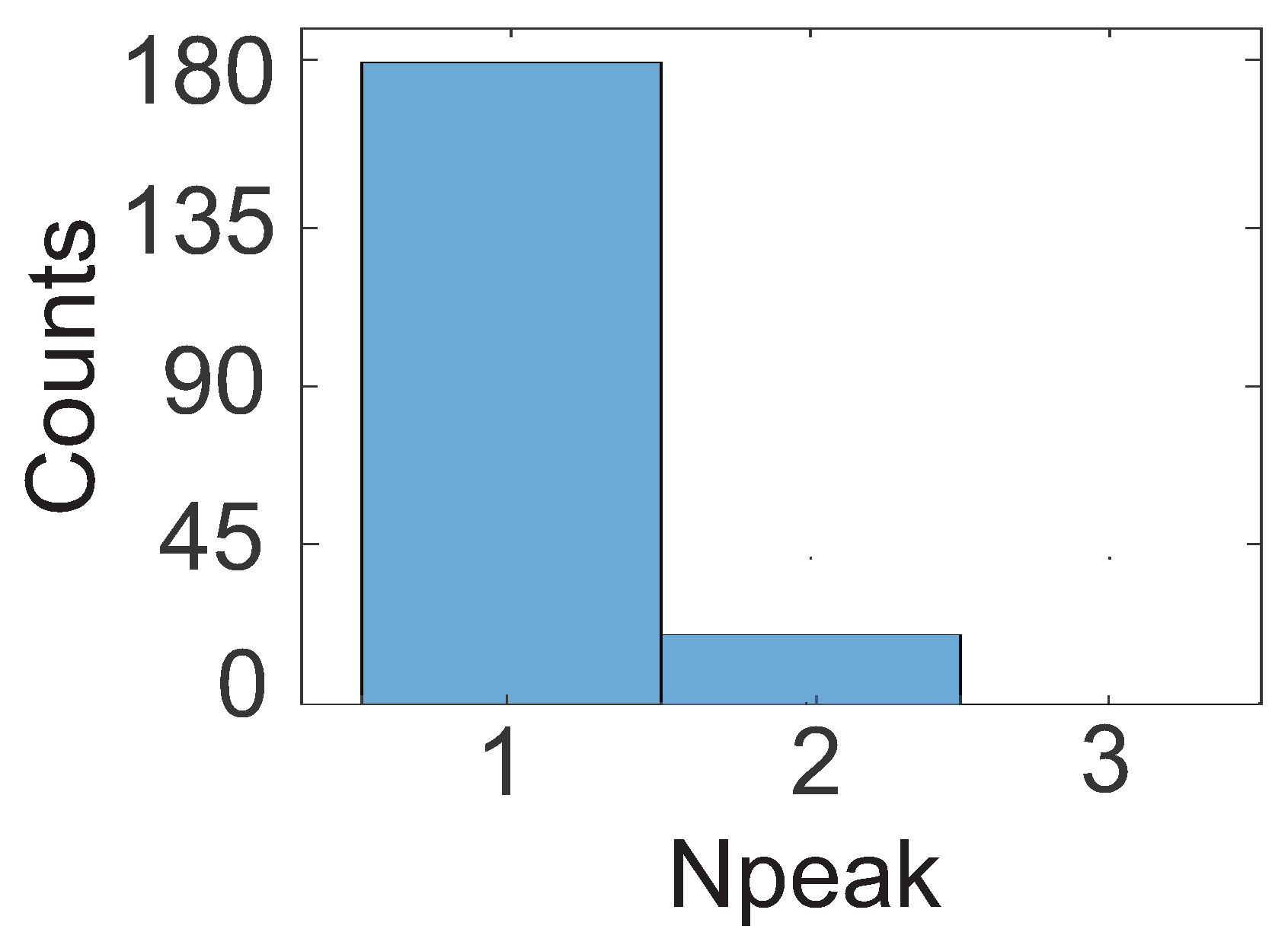
To ensure a reliable excitation source, we conducted 200 LLE iterations along the chosen $(\mathsf{\Delta }, {\left|S\right|}^2)$ path and consistently observed a single intensity peak at the end of each run (Npeak = 1), evidencing deterministic DKS generation (Figure 6).

To evaluate the repeatability of DKS generation in the presence of fabrication variability, we carried out a Monte Carlo study based on the LLE. Because the LLE is parametrized by effective cavity quantities rather than explicit geometric dimensions (gap or width), we represent manufacturing tolerances through the intrinsic resonator parameters set by the geometry: the radius, $\alpha$, ${\beta }_2$ and $\theta$.

In each realization, the parameter set was drawn independently from uniform distributions over the tolerance-based ranges listed in

Table 2. Range of DCM intrinsic parameters.

Parameters	Range
radius	[99, 103] [$\mathrm{\mu }$m]
$\alpha$	[$1.594\times {10}^{-3}$, $1.6113\times {10}^{-3}$]
$\theta$	[$6.38\times {10}^{-4}$, $6.49\times {10}^{-4}$]
${\beta }_2$	[$-6.8\times {10}^{-26}$, $-3.8\times {10}^{-26}$] [${\mathrm{s}}^2{\mathrm{m}}^{-1}$]

. For every sampled set, we solved the LLE using the same excitation and tuning protocol as for the nominal device, and we determined whether a DKS state was obtained using the same identification criterion applied throughout the manuscript.

For the DCM configuration analyzed here, the Monte Carlo ensemble produces DKS formation in 178 of 200 realizations, corresponding to a success probability of $89\%$ under concurrent tolerance-level perturbations.

Figure 7 shows the resulting histogram of $N_{\mathrm{peak}}$, which is predominantly concentrated in the range classified as DKS. Overall, these statistics indicate that the chosen operating point is resilient to fabrication-induced parameter variations and justify the repeatability premise adopted in the subsequent sensing and classification analyses.

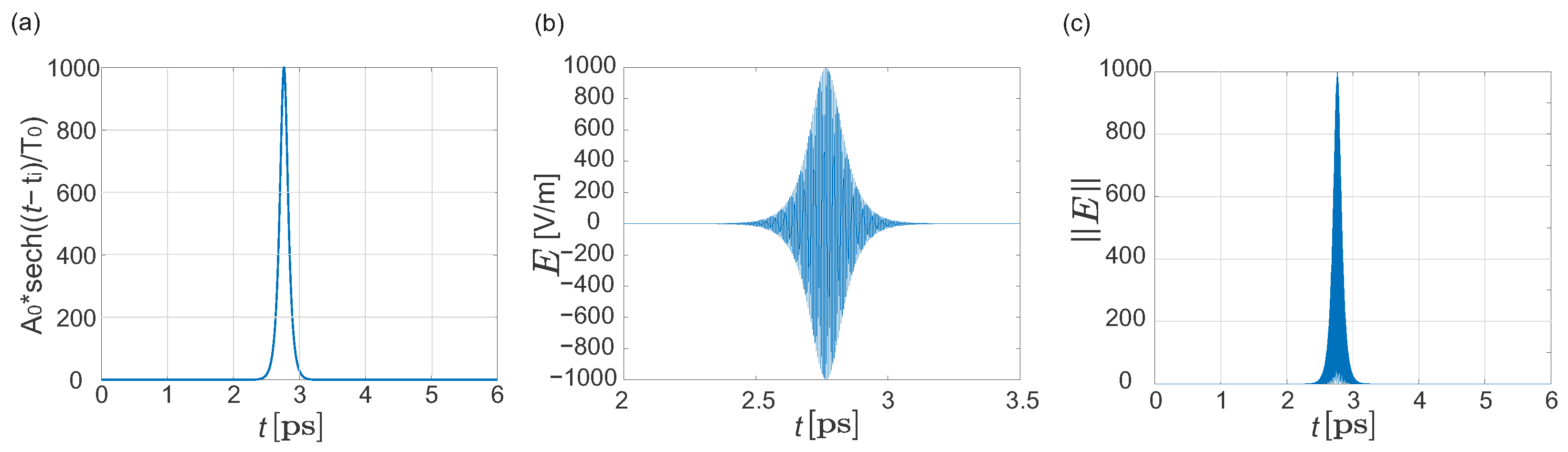
We then obtained the temporal parameters $T_0$ and $T_i$ directly from Figure 5c and set $A_0$ from the driving power (47.6 mW), which yields E-field amplitudes in the ${10}^3$–${10}^6$ [V/m] range. Figure 8 depicts the analytical DKS envelope later used as FEM excitation and the corresponding $\parallel E\parallel$ observable employed for data generation.

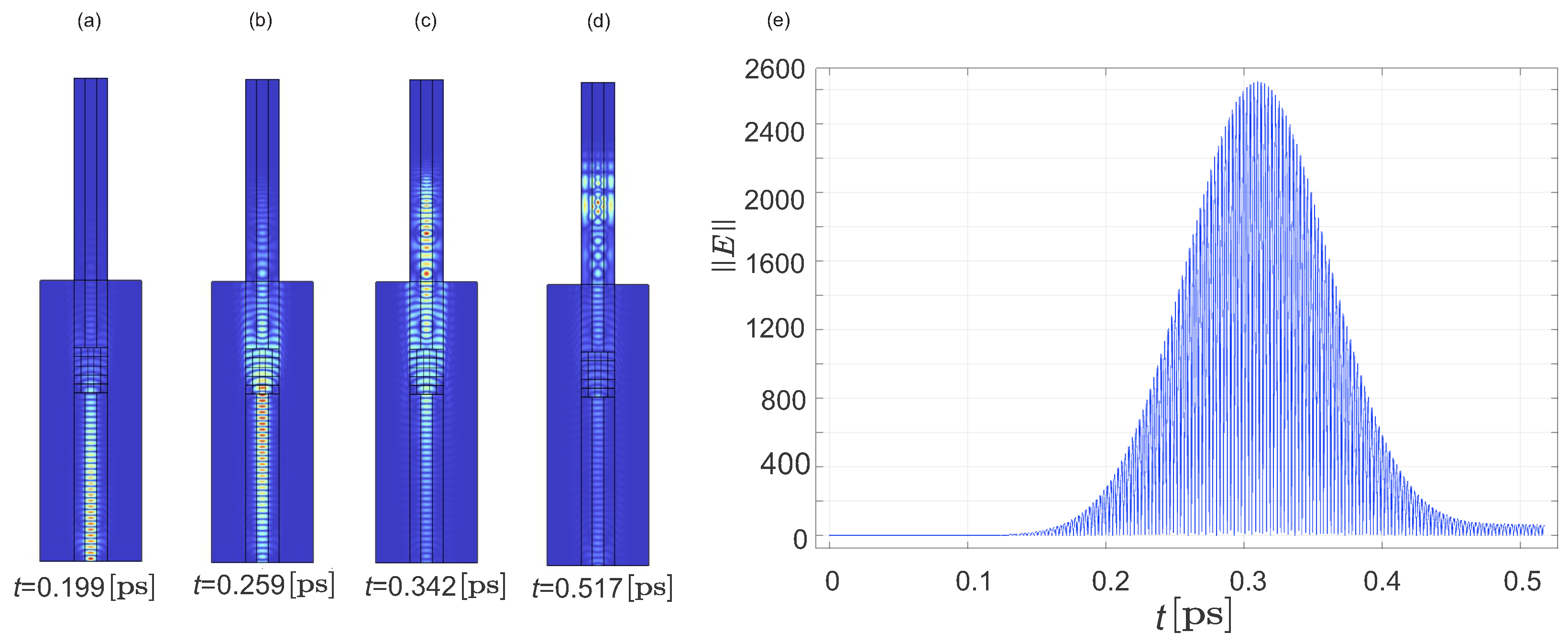
With this excitation, we solve the full-wave Maxwell equations in the ${\mathrm{distilled-water/TiO}}_2$ interaction region using the FEM method. Figure 9 presents representative time domain snapshots and the field magnitude $\parallel E\parallel$ recorded at the probe. When the field crosses a high-concentration area, its amplitude decreases and the apparent group delay increases (Figure 9e), consistent with the effective-index increase introduced by ${\mathrm{TiO}}_2$ and the associated dissipative and dispersive effects. This behavior underpins the separability of concentrations in the subsequent learning stage.

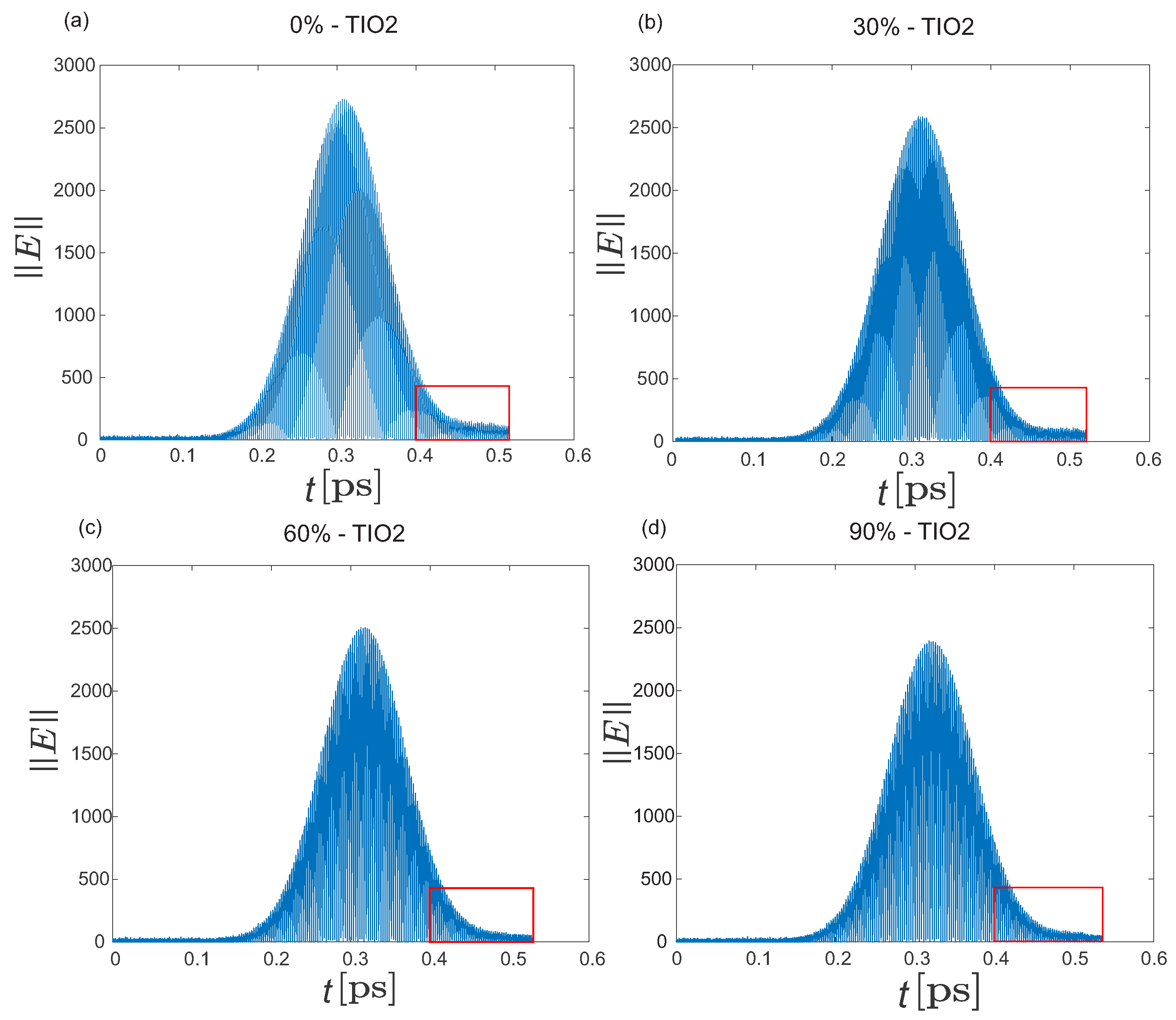
Figure 10 presents the temporal evolution of $\parallel E\parallel$ for ${\mathrm{TiO}}_2$ concentrations of 0%, 30%, 60%, and 90%, including additive Gaussian noise to emulate experimental perturbations.

As the nanoparticle concentration increases, a clear attenuation of the field amplitude and a pronounced temporal broadening of the pulse are observed, as highlighted by the red insets. These effects originate from the enhanced scattering and absorption introduced by the ${\mathrm{TiO}}_2$ nanoparticles, which locally modify the effective refractive index and introduce additional propagation losses in the medium. With increasing nanoparticle density, the DKS field undergoes stronger phase accumulation and dispersion, resulting in a reduced group velocity and an extended pulse duration. This combination of amplitude decay and phase shift confirms that $\parallel E\parallel$ carries concentration-dependent signatures detectable at the probe, validating the ability of the proposed system to encode nanoparticle-induced variations into measurable temporal features.

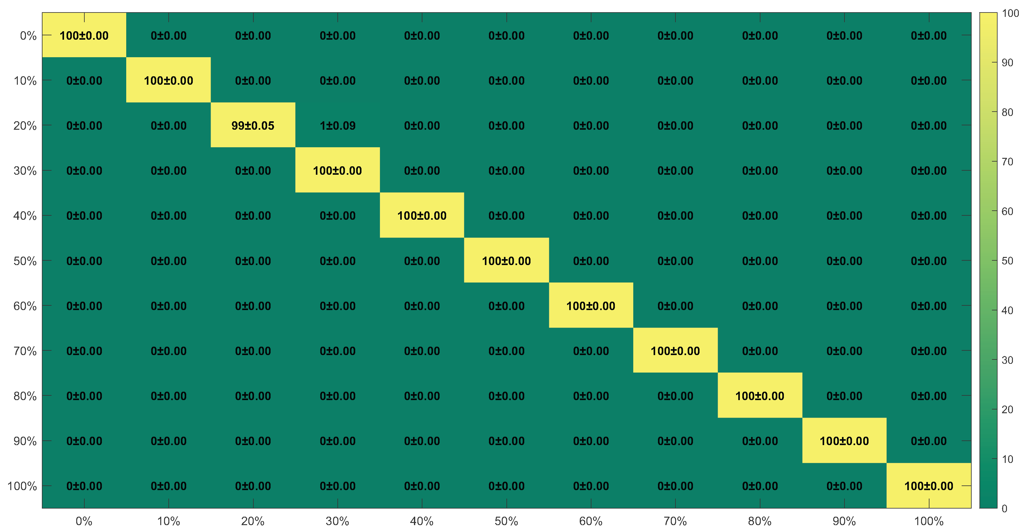
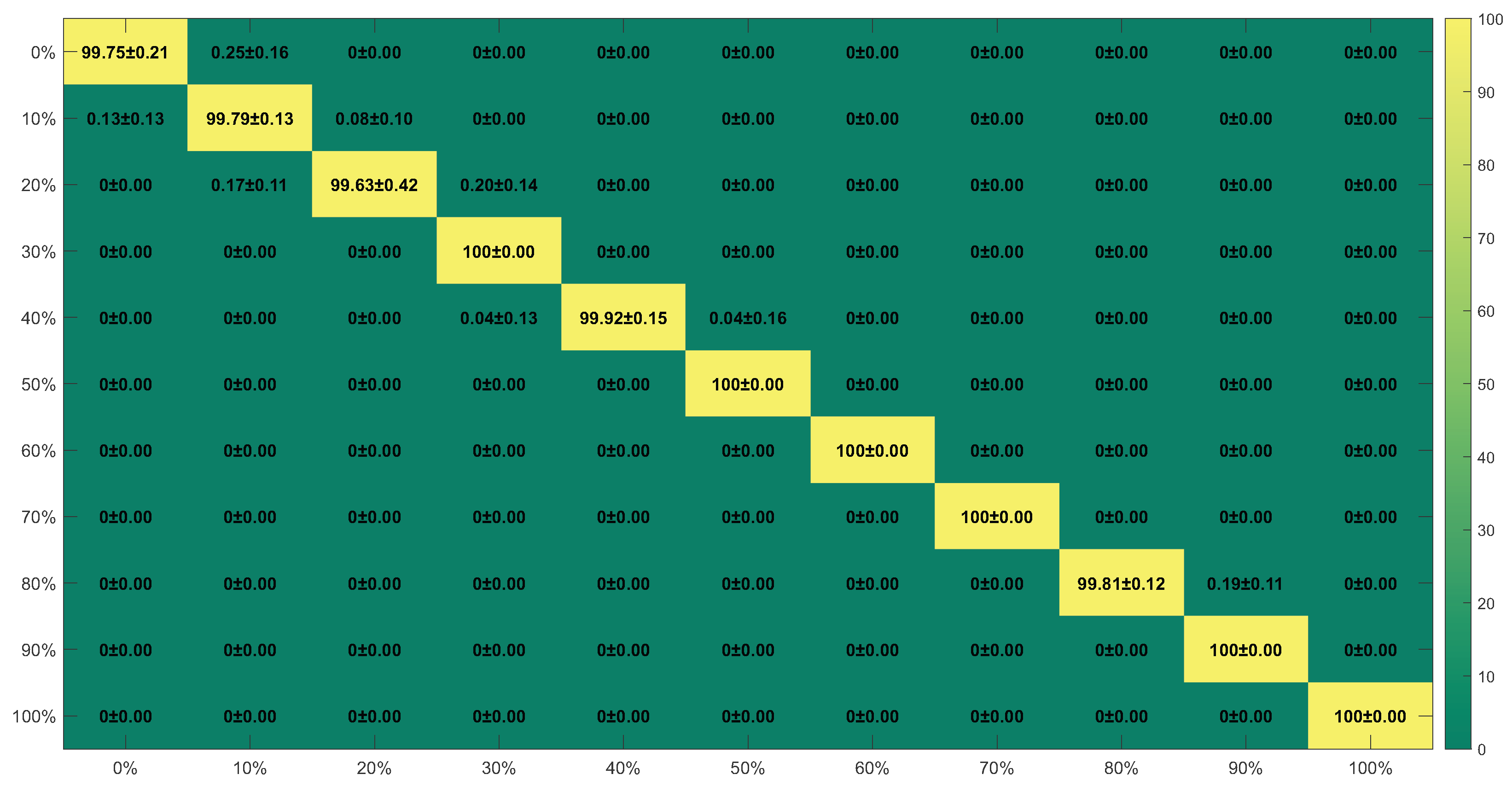
We next validate the automatic detection stage. The Transformer model achieves classification accuracies above 99% across all eleven ${\mathrm{TiO}}_2$ concentration levels, with only minimal deviations for the 10% and 60% cases (Figure 11). Similarly, the 1D-CNN baseline attains high performance (Figure 12), though slightly below the Transformer on average.

Table 3. Performance comparison of classification methods for automatic ${\mathrm{TiO}}_2$ nanoparticle detection.

Label	SVM	CNN-1D	1D ResNet	Transformer
0%	$97.80\pm 0.91$	$98.75\pm 0.21$	$100\pm 0$	$100\pm 0$
10%	$98.75\pm 0.53$	$99.79\pm 0.13$	$100\pm 0$	$100\pm 0$
20%	$99.44\pm 0.40$	$98.63\pm 0.42$	$100\pm 0$	$99.33\pm 0.01$
30%	$98.85\pm 0.17$	$100\pm 0$	$100\pm 0$	$100\pm 0$
40%	$94.90\pm 1.12$	$98.92\pm 0.15$	$100\pm 0$	$100\pm 0$
50%	$74.82\pm 1.64$	$100\pm 0$	$100\pm 0$	$100\pm 0$
60%	$70.10\pm 2.76$	$100\pm 0$	$98.342\pm 0.994$	$100\pm 0$
70%	$82.91\pm 2.64$	$100\pm 0$	$98.337\pm 0.998$	$99\pm 0.05$
80%	$75.10\pm 2.76$	$99.81\pm 0.12$	$100\pm 0$	$100\pm 0$
90%	$67.66\pm 2.10$	$100\pm 0$	$100\pm 0$	$100\pm 0$
100%	$70.72\pm 1.31$	$100\pm 0$	$100\pm 0$	$100\pm 0$
Average %	$84.73\pm 1.48$	$99.71\pm 0.09$	$99.81\pm 0.08$	$99.84\pm 0.01$
Accuracy	$0.8465\pm 0.0039$	$0.9963\pm 0.00028$	$0.9968\pm 0.00027$	$0.9994\pm 0.00025$
Recall	$0.8465\pm 0.0039$	$0.9963\pm 0.00028$	$0.9968\pm 0.00027$	$0.9994\pm 0.00025$
F1	$0.8449\pm 0.0040$	$0.9962\pm 0.00029$	$0.9967\pm 0.00028$	$0.9993\pm 0.00026$
Cohen’s k	$0.8312\pm 0.0043$	$0.9961\pm 0.0003$	$0.9966\pm 0.00029$	$0.9992\pm 0.00027$
Time	$0.24\pm 0.01$ [s]	$1.06\pm 0.09$ [s]	$14.47\pm 1.12$ [s]	$0.793\pm 0.05$ [s]

summarizes the quantitative comparison with the SVM, CNN-1D, 1D-ResNet and Transformer models. While the SVM yields acceptable accuracy for some classes, its overall performance (84.73 ± 1.48%) remains limited by the intrinsic complexity of the wave-propagation signatures. In contrast, the deep-learning models exceed 99% mean accuracy (99.71 ± 0.09% for CNN-1D, 99.81 ± 0.08% for 1D-ResNet and 99.84 ± 0.01% for the Transformer), demonstrating their ability to discriminate between morphological variations in $\parallel E\parallel \left(t\right)$ that arise from different nanoparticle concentrations.

These results underscore the capacity of deep learning architectures to extract discriminative patterns embedded in optical field dynamics, thereby capturing subtle, concentration-dependent variations with high precision. The consistent performance of the Transformer across multiple Monte Carlo realizations, each trained and validated on independent dataset splits, further indicates strong generalization without observable overfitting. The low standard deviation observed across runs confirms that the learned representations remain stable in the presence of noise and small perturbations in the simulated data. This robustness provides a solid foundation for future extensions of the framework, including the incorporation of additional physical effects such as finer spatial partitioning within the Yamaguchi model, thermal fluctuations, particle motion, or time-varying nanoparticle concentrations. Although these aspects lie beyond the scope of the present study, the strong classification performance achieved here establishes a rigorous basis for advancing toward more complex and realistic photonic sensing scenarios.

The Transformer also exhibits favorable classification runtime, achieving an average inference time of (0.793 ± 0.05) s per sample, compared with CNN-1D (1.06 ± 0.09) s and 1D-ResNet (14.47 ± 1.12) s. Although the SVM yields faster inference on average, its substantially lower accuracy renders it unsuitable for the targeted detection fidelity. Overall, these results support the central hypothesis that combining DKS-based frequency-comb excitation, full-wave optical propagation, and deep sequence models enables high-accuracy, label-free detection of ${\mathrm{TiO}}_2$ concentrations.

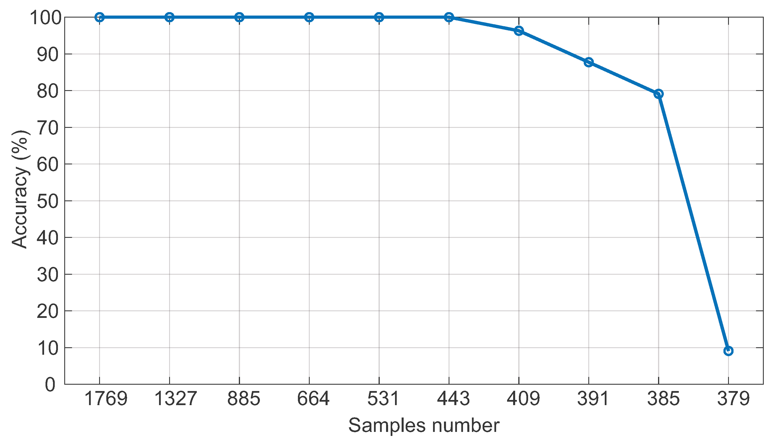
To assess the sensitivity of the automatic detection model to temporal sampling density, we investigated the impact of reducing the input sequence length. While the simulated $\parallel E\parallel$ traces are initially recorded with 1769 samples, we performed a systematic decimation study in which each trace was uniformly downsampled to N points and the Transformer was retrained under identical conditions. As shown in Figure 13, the classification accuracy remains essentially stable for $N\gtrsim 409$, and then decreases progressively as N is further reduced. Notably, even at $N=385$ samples, the model preserves a strong performance of ∼80% accuracy. These results demonstrate that the proposed classification approach is robust to substantial reductions in temporal sampling and does not require the full 1769 points resolution to maintain reliable concentration discrimination.

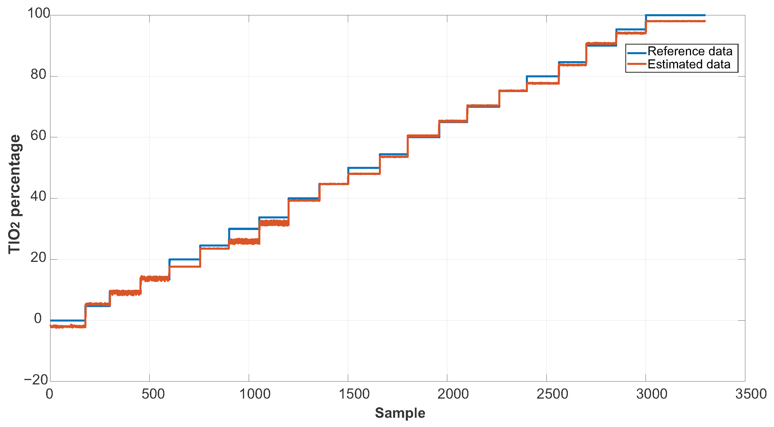
To evaluate the generalization capability of the proposed framework, the Transformer model was reconfigured from a classification setting to a regression setting, allowing continuous estimation of ${\mathrm{TiO}}_2$ concentration values. To support this regression task, the network architecture was adapted by replacing the final classification layers with a single-neuron regression head coupled to a regression loss function. In addition, the L2 regularization coefficient was reduced to $1\times {10}^{-4}$ and the dropout rate was lowered to 0.05 to better accommodate continuous-value prediction, while all remaining architectural components were preserved to maintain consistency with the classification model. Using this modified configuration, an auxiliary dataset was generated to complement the original training and evaluation data. In addition to the initial dataset comprising 11 uniformly spaced concentration levels spanning the full range from 0% to 100% with increments of 10%, intermediate concentration values uniformly offset by 5% across the same range were introduced. These additional samples enable a rigorous assessment of the model’s ability to interpolate concentration values within the studied domain.

The regression results demonstrate strong generalization performance, as illustrated in Figure 14, where the concentration values estimated by the model closely follow the reference validation data across the entire concentration range. The close agreement between the predicted and true concentration trajectories indicates that the model effectively captures the underlying relationship between the optical response and nanoparticle concentration. Quantitatively, this behavior is corroborated by the error metrics, with the root mean square error (RMSE) remaining consistently below 2% across all Monte Carlo realizations. The mean RMSE achieved is 1.73%, with a standard deviation of 1.14%, demonstrating both high accuracy and low variability, and confirming that the proposed framework learns a continuous and physically meaningful mapping between the optical signal features and ${\mathrm{TiO}}_2$ concentration.

4. Conclusions

This study presents a methodology for automatic and label-free detection of ${\mathrm{TiO}}_2$ nanoparticle concentrations that integrates deterministic DKS generation, full-wave optical propagation modeling, and deep learning models. A dual-coupled microring (DCM) architecture is used to delimit a stable operating region in which a constant-${\left|S\right|}^2$ trajectory bypasses chaotic regimes and ensures deterministic DKS generation. By combining frequency-comb excitation with physics-grounded propagation modeling and deep sequence analysis, the approach delivers accurate, label-free quantification of ${\mathrm{TiO}}_2$ from the probe’s optical signal. The resulting framework lays a solid foundation for extending frequency-comb spectroscopy to advanced biosensing applications and to other microresonator-based detection platforms.

The simulated propagation of the generated DKS pulse through the ${\mathrm{TiO}}_2$–water suspension reproduces the expected optical response: as concentration increases, the $\parallel E\parallel$ traces exhibit amplitude attenuation and temporal broadening, consistent with the effective-index and dissipative variations introduced by the nanoparticles. These effects demonstrate that the proposed modeling approach captures the fundamental physics governing the interaction between the DKS field and the medium. A 2D time-domain FEM model is employed under an extruded-geometry assumption $\left({\displaystyle \frac{\partial }{\partial z}}=0\right)$. This captures in-plane scattering/diffraction and re-coupling into the output waveguide, while neglecting out-of-plane diffraction. A subsequent validation step will assess the relevance of these 3D corrections via targeted 3D benchmarks or direct experimental measurements, depending on cost-benefit. The classification stage shows that deep learning models can effectively recognize these concentration-dependent distortions in the optical field. The Transformer achieved accuracies above 99% across all concentration levels, slightly surpassing the CNN-1D baseline and outperforming the SVM approach. The low variance obtained from the Monte Carlo validation confirms stable generalization and indicates that the stable performance across Monte Carlo realizations indicates that the classification relies on consistent, physically induced signal variations rather than dataset-specific correlations.

The physical tendencies observed in Figure 9 and Figure 10 align with theoretical expectations: higher ${\mathrm{TiO}}_2$ concentrations increase the effective refractive index and optical losses of the medium, producing measurable changes in the amplitude and temporal shape of $\parallel E\parallel$. These signatures are accurately captured by the learning models, supporting a consistent correspondence between the simulated photonic phenomena and the data-driven classification outcomes.

Although the present work focuses on two-dimensional propagation with $\partial /\partial z=0$ and a $5\times 5$ discretization of the Yamaguchi-based effective index, the methodology can be extended to three-dimensional configurations, finer spatial resolutions, or dynamic processes such as thermal fluctuations, particle motion, and time-varying concentrations. Future work will also address experimental validation and domain adaptation to bridge simulated and real optical data.

References

1. Chandoliya, R.; Sharma, S.; Sharma, V.; Joshi, R.; Sivanesan, I. Titanium Dioxide Nanoparticle: A Comprehensive Review on Synthesis, Applications and Toxicity. Plants 2024, 13, 2964. [Google Scholar] [CrossRef]
2. Zhang, Z.; Li, D.; Wang, X.; Wang, Y.; Lin, J.; Jiang, S.; Wu, Z.; He, Y.; Gao, X.; Zhu, Z.; et al. Rapid detection of viruses: Based on silver nanoparticles modified with bromine ions and acetonitrile. Chem. Eng. J. 2022, 438, 135589. [Google Scholar] [CrossRef]
3. Liang, Q.; Chan, Y.-C.; Toscano, J.; Bjorkman, K.K.; Leinwand, L.A.; Parker, R.; Nozik, E.S.; Nesbitt, D.J.; Ye, J. Breath analysis by ultra-sensitive broadband laser spectroscopy detects SARS-CoV-2 infection. J. Breath Res. 2023, 17, 036001. [Google Scholar] [CrossRef]
4. Li, X.; Yang, T.; Li, S.; Wang, D.; Song, Y.; Zhang, S. Raman spectroscopy combined with principal component analysis and k nearest neighbour analysis for non-invasive detection of colon cancer. Laser Phys. 2016, 26, 035702. [Google Scholar] [CrossRef]
5. Luo, R.; Popp, J.; Bocklitz, T. Deep Learning for Raman Spectroscopy: A Review. Analytica 2022, 3, 287–301. [Google Scholar] [CrossRef]
6. Li, J.; Dukes, P.; Lee, W.; Sarkis, M.; Vo-Dinh, T. Machine Learning Using Convolutional Neural Networks for SERS Analysis of Biomarkers in Medical Diagnostics. J. Raman Spectrosc. 2022, 53, 2044–2057. [Google Scholar] [CrossRef] [PubMed]
7. Ikponmwoba, E.; Ukorigho, O.; Moitra, P.; Pan, D.; Gartia, M.; Owoyele, O. A Machine Learning Framework for Detecting COVID-19 Infection Using Surface-Enhanced Raman Scattering. Biosensors 2022, 12, 589. [Google Scholar] [CrossRef] [PubMed]
8. Kippenberg, T.J.; Gaeta, A.L.; Lipson, M.; Gorodetsky, M.L. Dissipative Kerr solitons in optical microresonators. Science 2018, 361, 1095–9203. [Google Scholar] [CrossRef]
9. Wang, W.; Wang, L.; Zhang, W. Advances in soliton microcomb generation. Adv. Photonics 2020, 2, 034001. [Google Scholar] [CrossRef]
10. Calvo-Salcedo, A.F.; Guerrero González, N.; Jaramillo-Villegas, J.A. Dynamic Spectrum Assignment in Passive Optical Networks Based on Optical Integrated Microring Resonators Using Machine Learning and a Routing, Modulation Level, and Spectrum Assignment Method. Appl. Sci. 2023, 13, 13294. [Google Scholar] [CrossRef]
11. Ahmeti, F.; Teker, K. A model for an Optical Ring Micro resonator towards Nanoparticle Detection. In Proceedings of the 11th Annual TechConnect World Innovation Conference and Expo, Held Jointly with the 20th Annual Nanotech Conference and Expo, and the 2017 National SBIR/STTR Conference, Washington, DC, USA, 14–17 May 2017; Optica Publishing Group: Washington, DC, USA, 2017; pp. 254–257. [Google Scholar]
12. Bao, C.; Yuan, Z.; Wu, L.; Suh, M.-G.; Wang, H.; Lin, Q.; Vahala, K. Architecture for microcomb-based GHz-mid-infrared dual-comb spectroscopy. Nat. Commun. 2021, 12, 6573. [Google Scholar] [CrossRef]
13. Stern, L.; Stone, J.R.; Kang, S.; Cole, D.C.; Suh, M.-G.; Fredrick, C.; Newman, Z.; Vahala, K.; Kitching, J.; Diddams, S.A.; et al. Direct Kerr frequency comb atomic spectroscopy and stabilization. Sci. Adv. 2020, 6, eaax6230. [Google Scholar] [CrossRef]
14. Dutt, A.; Joshi, C.; Ji, X.; Cardenas, J.; Okawachi, Y.; Luke, K.; Gaeta, A.L.; Lipson, M. On-chip dual-comb source for spectroscopy. Sci. Adv. 2018, 4, e1701858. [Google Scholar] [CrossRef]
15. Bouchand, R.; Weng, W.; Lucas, E.; Karpov, M.; Pfeiffer, M.H.P.; Liu, J.; Guo, H.; Anderson, M.H.; Raja, A.S.; Lukashchuk, A.; et al. Dissipative Kerr solitons in photonic chip-based microresonators. In Proceedings of the Optical Fiber Communication Conference (OFC), San Diego, CA, USA, 11–15 March 2018; Optica Publishing Group: Washington, DC, USA, 2018. [Google Scholar] [CrossRef]
16. Jaramillo-Villegas, J.A.; Xue, X.; Wang, P.H.; Leaird, D.E.; Weiner, A.M. Deterministic single soliton generation and compression in microring resonators avoiding the chaotic region. Opt. Express 2015, 23, 9618. [Google Scholar] [CrossRef] [PubMed]
17. Zhang, B.; Chen, N.; Lu, X.; Chen, Y.; Zhang, X.; Xu, J. Dissipative Kerr single soliton generation with extremely high probability via spectral mode depletion. Front. Optoelectron. 2022, 15, 48. [Google Scholar] [CrossRef] [PubMed]
18. Bao, C.; Xuan, Y.; Leaird, D.E.; Wabnitz, S.; Qi, M.; Weiner, A.M. Spatial mode-interaction induced single soliton generation in microresonators. Optica 2017, 4, 1011–1015. [Google Scholar] [CrossRef]
19. Moille, G.; Leonhardt, M.; Paligora, D.; Englebert, N.; Leo, F.; Fatome, J.; Srinivasan, K.; Erkintalo, M. Parametrically driven pure-Kerr dissipative solitons in a chip-integrated microcavity. Nat. Photonics 2024, 18, 617–624. [Google Scholar] [CrossRef]
20. Xue, X.; Zheng, X.; Zhou, B. Super-efficient temporal solitons in mutually coupled optical cavities. Nat. Photonics 2019, 13, 616–622. [Google Scholar] [CrossRef]
21. Diddams, S.A.; Vahala, K.; Udem, T. Optical frequency combs: Coherently uniting the electromagnetic spectrum. Science 2020, 369, eaay3676. [Google Scholar] [CrossRef]
22. Marti, L.; Vasco, J.P.; Savona, V. Slow-light enhanced frequency combs and dissipative Kerr solitons in silicon coupled-ring microresonators in the telecom band. OSA Contin. 2021, 4, 1247–1257. [Google Scholar] [CrossRef]
23. Wu, Z.; Gao, Y.; Zhang, T.; Dai, J.; Xu, K. Switching dynamics of dissipative cnoidal waves in dual-coupled microresonators. Opt. Express 2021, 29, 42369–42383. [Google Scholar] [CrossRef]
24. Vladimirov, A.G.; Tlidi, M.; Taki, M. Dissipative soliton interaction in Kerr resonators with high-order dispersion. Phys. Rev. A 2021, 103, 063505. [Google Scholar] [CrossRef]
25. Chen, X.; Wu, X.; Chen, C.; Luo, C.; Shi, Y.; Li, Z.; Lv, X.; Chen, C.; Su, J.; Wu, L. Raman spectroscopy combined with a support vector machine algorithm as a diagnostic technique for primary Sjögren’s syndrome. Sci. Rep. 2023, 13, 5137. [Google Scholar] [CrossRef] [PubMed]
26. Ember, K.; Daoust, F.; Mahfoud, M.; Dallaire, F.; Zamani, E.; Tran, T.; Plante, A.; Diop, M.-K.; Nguyen, T.; St-Georges-Robillard, A.; et al. Saliva-based detection of COVID-19 infection in a real-world setting using reagent-free Raman spectroscopy and machine learning. medRxiv 2021. [Google Scholar] [CrossRef] [PubMed]
27. Kazemzadeh, M.; Hisey, C.L.; Zargar-Shoshtari, K.; Xu, W.; Broderick, N.G.R. Deep convolutional neural networks as a unified solution for Raman spectroscopy-based classification in biomedical applications. Opt. Commun. 2022, 510, 127977. [Google Scholar] [CrossRef]
28. Zhang, W.; Feng, W.; Cai, Z.; Wang, H.; Yan, Q.; Wang, Q. A deep one-dimensional convolutional neural network for microplastics classification using Raman spectroscopy. Vib. Spectrosc. 2023, 124, 103487. [Google Scholar] [CrossRef]
29. Calvo-Salcedo, A.F.; Guerrero González, N.; Jaramillo-Villegas, J.A. Obtaining Dissipative Kerr Solitons Deterministically Using Dual-Coupled Microresonators and a Simple Frequency Sweep. Appl. Sci. 2024, 14, 10819. [Google Scholar] [CrossRef]
30. Malitson, I.H. Interspecimen comparison of the refractive index of fused silica. J. Opt. Soc. Am. 1965, 55, 1205–1209. [Google Scholar] [CrossRef]
31. Polyanskiy, M.N. Refractiveindex.info Database of Optical Constants. Sci. Data 2024, 11, 94. [Google Scholar] [CrossRef] [PubMed]
Figure 1. Block diagram for automatic TiO 2 detection with an DCM and machine learning.
Technologies 14 00065 g001
Figure 2. (a) DCM structure. (b) Parametric space ( Δ ,   S 2 ) . (c) Path in the ( Δ ,   S 2 ) for the DKS generation. (d) DKS spectrum. (e) DKS intensity.
Technologies 14 00065 g002
Figure 3. Temporal characterization of DKS.
Technologies 14 00065 g003
Figure 4. (a) Simulation setup. (b) Geometric design and meshing for the FEM method. (c) Design dimensions. (d) Cell for implementing the Yamaguchi model. (e) Finite-element mesh.
Technologies 14 00065 g004
Figure 5. (a) Parametric space ( Δ ,   S 2 ) for the DCM. (b) Selected path for DKS generation in the ( Δ ,   S 2 ) plane. (c) Optical intensity of the DKS. (d) Optical spectrum of the DKS.
Technologies 14 00065 g005
Figure 6. Monte Carlo experiment for deterministic DKS generation.
Technologies 14 00065 g006
Figure 7. Monte Carlo histogram of the number of peaks (Npeak) for 200 simulations.
Technologies 14 00065 g007
Figure 8. (a) DKS contour defined by the sech2 function. (b) Electric field E using the defined contour. (c) Electric field norm E .
Technologies 14 00065 g008
Figure 9. (ad) FEM snapshots at different time instants. (e) Temporal evolution of the electric field norm E at the measurement probe.
Technologies 14 00065 g009
Figure 10. (a) Electric field norm E for 0% TiO 2 . (b) 30% TiO 2 . (c) 60% TiO 2 . (d) 90% TiO 2 .
Technologies 14 00065 g010
Figure 11. Confusion matrix for Transformer-based TiO 2 nanoparticle classification.
Technologies 14 00065 g011
Figure 12. Confusion matrix for CNN-1D-based TiO 2 nanoparticle classification.
Technologies 14 00065 g012
Figure 13. Classification accuracy versus input-signal resolution.
Technologies 14 00065 g013
Figure 14. Regression-based estimation of TiO 2 concentration.
Technologies 14 00065 g014