Adaptive High-Order Sliding Mode Control for By-Wire Ground Vehicle Systems

Abstract

This study focuses on the design and implementation of an Adaptive High-Order sliding mode control for by-wire ground vehicle systems. The controller integrates advanced technologies such as Active Front Steering (AFS) and Rear Torque Vectoring (RTV), aimed at enhancing vehicle dynamics. However, lateral velocity remains one of the most challenging variables to measure, even in modern vehicles. To address this limitation, a High-Order Sliding Mode (HOSM)-based observer with adaptive gains is proposed. The HOSM observer provides critical information for the operation of the dynamic controller, ensuring the tracking of desired references. Compared with traditional observers, the proposed adaptive HOSM observer achieves finite-time convergence of state estimation errors and exhibits enhanced robustness against external disturbances, as confirmed through simulation results. The adaptive gains dynamically adjust the system parameters, enhancing its precision and flexibility under changing environmental conditions. This dynamic approach ensures efficient and reliable performance, enabling the system to respond effectively to complex scenarios. The stability of the dynamic HOSM controller with adaptive gain is analyzed through a Lyapunov-based approach, providing solid theoretical guarantees. Its performance is evaluated using detailed simulations conducted in CarSim 2017 software. The simulation results demonstrate that the proposed controller is highly effective in ensuring accurate trajectory tracking.

1. Introduction

In contemporary vehicles, a variety of electronic subsystems, collectively referred to as by-wire systems, have been incorporated to enhance occupant safety by supplanting traditional mechanical and hydraulic components. Key subsystems crucial for passenger protection include those involved in controlling the vehicle’s posture, such as the steering and braking mechanisms. Within the steering domain, steer-by-wire (SBW) technology broadens the spectrum of control capabilities, encompassing Active Front Steering (AFS), which adjusts the driver’s steering input to counteract external forces acting on the vehicle. Similarly, by-wire braking systems or active differential mechanisms facilitate the implementation of a Rear Torque Vectoring (RTV) subsystem, which allocates torque to the rear axle by inducing a yaw moment, thereby improving vehicle stability and handling.

This research centers on the development of a dynamic HOSM controller with adaptive gains, designed for ground vehicles equipped with Active Front Steering (AFS) and Rear Torque Vectoring (RTV) systems. The proposed dynamic control strategy leverages adaptive gains to achieve precise regulation of yaw and lateral dynamics, enabling accurate trajectory tracking. The controller is specifically designed to ensure the vehicle adheres to the desired trajectory, even in the presence of external disturbances or dynamic variations within the system [1].

Previous studies by the authors have focused on developing active controllers capable of addressing parameter variations, such as tire–road friction coefficients, as well as external disturbances like wind [2,3,4]. Other researchers, including [5,6], have explored the design of active controllers incorporating AFS and RTV systems, albeit without accounting for parametric variations. However, neglecting parameter variations, such as changes in cornering stiffness, vehicle mass distribution, or moment of inertia, can significantly degrade the accuracy of lateral velocity and yaw rate estimation, leading to control performance deterioration. This highlights the importance of designing observers and controllers that explicitly account for parameter variations in order to ensure robustness and high tracking accuracy under realistic operating conditions. In this context, recent advances in nonlinear control design, particularly techniques aimed at estimating external disturbances, have been comprehensively reviewed in [7,8,9,10,11]. Notably, recent works such as [12] introduce robust sliding mode control schemes capable of handling actuator faults and time-varying delays within a semi-Markovian jump framework, thereby illustrating the efficacy of state-estimation methodologies in managing complex uncertainties in sliding mode control. Furthermore, [13] examines the challenge of vehicle attitude control via AFS, employing neural networks to achieve real-time estimation of unknown nonlinearities, while [14] addresses both structured and unstructured uncertainties through estimation techniques followed by active disturbance rejection control. In [15], advanced methods such as radial basis function neural networks are utilized to mitigate the effects of external disturbances on vehicle dynamics.

In this paper, we introduce a significant innovation based on the latest developments in the field. This study simultaneously addresses three main aspects:

• A HOSM observer with adaptive gains is designed to ensure accurate estimation of lateral velocity for ground vehicles.
• A Dynamic HOSM controller with adaptive gains equipped with AFS and RTV systems. The controller incorporates an HOSM-based observer.
• An evaluation of the proposed control strategy was conducted using the CarSim simulation platform.

A review of the existing literature indicates the absence of studies that address the development of a Dynamic HOSM controller with adaptive gains specifically designed for ground vehicles to ensure that their lateral and yaw dynamics closely follow a reference trajectory. The dynamic control approach proposed in this work is subjected to validation through the implementation of a double-step maneuver, a challenging test scenario. This evaluation is conducted using the CarSim simulation platform, known for its detailed and accurate representation of vehicle dynamics. Although real-world experiments could provide further practical insights, this study primarily emphasizes the methodological framework rather than physical implementation on actual vehicles.

The HOSM methodology, while serving as a design tool rather than the core focus of this work, was initially introduced in [16]. Its key advantage lies in mitigating the chattering phenomenon caused by high-frequency switching on the sliding surface [17]. This represents a significant advancement over conventional first-order sliding mode techniques [18,19]. Moreover, HOSM facilitates the design of sliding mode surfaces with a relative degree greater than one [20].

Although adaptive control techniques have proven effective in a variety of applications, their use in complex systems characterized by dynamic environments and high levels of uncertainty remains relatively limited. In unmanned aerial vehicles (UAVs), for instance, adaptive control has only recently been investigated as a strategy to address unpredictable factors such as wind disturbances and payload fluctuations [21,22]. Similarly, in the automotive domain, the application of adaptive control for real-time suspension and steering systems has been comparatively scarce, despite its significant potential to enhance ride comfort and vehicle stability [23,24]. This gap in application underscores the need for further research to fully harness the capabilities of adaptive control in improving system robustness.

The paper is structured as follows: Section 2 presents the vehicle dynamics model, providing the equations and assumptions underpinning the system’s behavior. Section 3 addresses the design of a nonlinear robust output using adaptive gain, focusing on lateral velocity. Section 4 introduces the active dynamic control system, which incorporates the adaptive gain. Section 5 discusses the simulation results, validating the controller’s performance through simulations conducted in CarSim. Finally, Section 6 concludes the paper with a summary of the findings and contributions.

2. Mathematical Model of the Vehicle Dynamics

The model adopted in this work prioritizes the characterization of the dominant lateral and yaw dynamics. Consequently, it neglects secondary effects such as body roll and higher-order nonlinearities in tire forces. Their omission allows for reduced model complexity, enabling a more tractable derivation of the adaptive HOSM observer and controller while preserving the accuracy required for control design. This modeling choice is validated through simulation using the CarSim model, confirming that the adopted simplifications do not compromise the estimation or tracking performance. Previous works, such as [25,26], have employed Active Front Steering (AFS) as a control mechanism by introducing incremental adjustments to the steering angle ${\delta }_c$. Furthermore, the yaw moment $M_z$ is leveraged as an additional control input to modulate longitudinal forces via active braking. Consequently, the mathematical model describing the ground vehicle’s dynamics is expressed as follows:

$$\begin{array}{cc}\hfill m({\dot{v}}_x-v_y{\omega }_z)& ={\mu }_x(F_{x,f}+F_{x,r})+F_{d,x}=m{a}_x\hfill \\ \hfill m({\dot{v}}_y+v_x{\omega }_z)& ={\mu }_y(F_{y,f}+F_{y,r})+F_{d,y}=m{a}_y\hfill \\ \hfill J_z{\dot{\omega }}_z& ={\mu }_y(l_f{F}_{y,f}-l_r{F}_{y,r})+M_z+M_{d,z}\hfill \\ \hfill {\dot{\alpha }}_z& ={\omega }_z\hfill \end{array}$$

(1)

The variables $v_x$ and $v_y$ correspond to the longitudinal and lateral velocities of the vehicle at its center of mass, respectively, while ${\omega }_z$ represents the yaw rate, and ${\alpha }_z$ denotes the yaw angle. The vehicle’s mass is indicated by m, and $J_z$ represents its moment of inertia. The distances from the center of mass to the front and rear axles are denoted by $l_f$ and $l_r$, respectively. The coefficients ${\mu }_x$ and ${\mu }_y$ characterize the tire–road friction in the longitudinal and lateral directions. Longitudinal forces acting on the front and rear tires are represented by $F_{x,f}$ and $F_{x,r}$, while $F_{y,f}$ and $F_{y,r}$ correspond to the lateral forces on the front and rear tires. The yaw moment generated by the vehicle is denoted as $M_z$. Additionally, external disturbance forces, such as wind, are described by $F_{d,x}$ and $F_{d,y}$, with $M_{d,z}$ representing the associated torque.

The lateral forces discussed in this work are modeled using Pacejka’s magic formula:

$$F_{y,j}\left({\alpha }_j\right)=D_{j}sin(C_{j}arctan\left(B_j{\alpha }_j)\right),j=f,r$$

(2)

where $B_j$, $C_j$, and $D_j$ are parameters obtained through experimental analysis [27] and are directly influenced by the slip angle of the front tires, which is defined as follows:

$${\alpha }_f=({\delta }_d+{\delta }_c)-(v_y+l_f{\omega }_z)/v_x;{\alpha }_r=-(v_y-l_r{\omega }_z)/v_x$$

In this context, ${\delta }_d$ represents the road wheel angle dictated by the driver, while ${\delta }_c$ corresponds to the Active Front Steering (AFS) adjustment applied by the control system.

It is worth noting that if the function $F_{y,f}$ is not globally invertible, as is the case when the tire characteristic (2) is considered, one can still invert $F_{y,f}$ locally, namely for ${\alpha }_f\in [-{\alpha }_{f,max}, {\alpha }_{f,max}]$, where $\pm {\alpha }_{f,max}$ are the values of ${\alpha }_f$ corresponding to the minimum/maximum values of $F_{y,f}$. For the other values of ${\alpha }_f$, one can formally associate with ${\alpha }_f\notin [-{\alpha }_{f,max}, {\alpha }_{f,max}]$ the minimum/maximum value $F_{y,f}\left({\alpha }_f\right)=\pm F_{y,f}\left({\alpha }_{f,max}\right)$, which, when inverted, gives the value ${\alpha }_f=({\delta }_d+{\delta }_c)-{\displaystyle \frac{v_y+l_f{\omega }_z}{v_x}}=\pm {\alpha }_{f,max}$.

Summarizing, one can consider the following inversion rule [2,3].

$${\delta }_c=\left\{\begin{array}{cc}-{\delta }_d+{\displaystyle \frac{v_y+l_f{\omega }_z}{v_x}}+F_{y,f}^{-1}\left(F_{y,f,0}\right)\hfill & \mathrm{if}{\alpha }_f\in [-{\alpha }_{f,max}, {\alpha }_{f,max}],\hfill \\ -{\delta }_d+{\displaystyle \frac{v_y+l_f{\omega }_z}{v_x}}\pm {\alpha }_{f,max}\hfill & \mathrm{otherwise}.\hfill \end{array}\right.$$

for a given value $F_{y,f,0}$.

Since the lateral force $F_{y,f}({\delta }_d+{\delta }_c)$ is considered an invertible function, it enables the formulation of the following control input:

$${\Delta }_f=F_{y,f}({\delta }_d+{\delta }_c)-F_{y,f}\left({\delta }_d\right).$$

By incorporating the control input ${\Delta }_f$ into the equations governing the lateral velocity and yaw rate dynamics of the ground vehicle model (1), and under the assumption that $F_{x,f}=0$ and $F_{x,r}=0$, i.e., $F_{x,f}+F_{x,r}=0$, viz., no acceleration/deceleration is produced during the vehicle maneuvers, the vehicle dynamics (1) can be re-expressed as follows:

$$\begin{array}{cc}\hfill {\dot{v}}_x& =v_y{\omega }_z+{\displaystyle \frac{1}{m}}{F}_{d,x},\hfill \\ \hfill {\dot{v}}_y& =-v_x{\omega }_z+{\displaystyle \frac{{\mu }_y}{m}}\left(F_{y,f}\left({\delta }_d\right)+F_{y,r}\right)+{\displaystyle \frac{{\mu }_y}{m}}{\Delta }_f+{\displaystyle \frac{1}{m}}{F}_{d,y},\hfill \\ \hfill {\dot{\omega }}_z& ={\displaystyle \frac{{\mu }_y}{J_z}}\left(l_f{F}_{y,f}\left({\delta }_d\right)-l_r{F}_{y,r}\right)+{\displaystyle \frac{{\mu }_y}{J_z}}{l}_f{\Delta }_f+{\displaystyle \frac{1}{J_z}}{M}_z+{\displaystyle \frac{1}{J_z}}{M}_{d,z}.\hfill \end{array}$$

(3)

Assumption 1.

The external disturbance forces and moments acting on the vehicle model (1), denoted as $F_{d,x}$, $F_{d,y}$, and $M_{d,z}$, are bounded within predefined limits.

Assumption 1 establishes that the external disturbance forces and moment, denoted by $F_{d,x}$, $F_{d,y}$, and $M_{d,z}$, are constrained within certain limits. These conditions are essential in practical scenarios, as it is presumed that such disturbances are bounded and do not undergo infinitely rapid variations in velocity.

3. Design of an HOSM Observer with Adaptive Gain

The lateral velocity $v_y$ is generally not available from direct measurements. Therefore, the adaptive gain HOSM observer developed in this section operates under the assumption that $a_x$, $a_y$, ${\omega }_z$, and $v_x$ are measurable signals, while $v_y$ must be reconstructed through observation. This assumption is fully consistent with modern vehicles, where electronic stability control systems and integrated sensor networks provide reliable access to the aforementioned variables. To rigorously ensure the finite-time convergence properties of the observer, the following assumption is introduced:

Assumption 2.

Throughout a maneuver, the yaw angular velocity ${\omega }_z$ is maintained as nonzero and bounded for all $t\ge t_0$, such that $0<{\omega }_{z,min}\le |{\omega }_z|\le {\omega }_{z,max}$.

Assumption 2 provides a sufficient condition to guarantee the stability and finite-time convergence of the observer. When the vehicle follows a perfectly straight path, i.e., ${\omega }_z=0$, the lateral velocity $v_y$ naturally approaches zero. In such situations, observing $v_y$ is not essential, as it contributes negligibly to the vehicle’s motion. Conversely, when ${\omega }_z\ne 0$, the lateral velocity $v_y$ becomes nonzero and must be reconstructed through observation to ensure accurate state feedback. To address this requirement, a reduced-order adaptive gain HOSM observer is designed to reconstruct $v_y$ in finite time.

For this purpose, we adopt the following notation: ${⌊·⌉}^{1/2}={|·|}^{1/2}{⌊·⌉}^0$, ${⌊·⌉}^0=\mathrm{sign}(·)$

Theorem 1.

Under Assumption 2, and assuming that the signals $a_x$, $a_y$, ${\omega }_z$, and $v_x$ are measurable, the HOSM observer with adaptive gains is defined as follows:

$$\begin{array}{cc}\hfill {\dot{\widehat{v}}}_x& ={\widehat{v}}_y{\omega }_z+a_x+{\gamma }_1\left(t\right)|{\omega }_z|{⌊{\tilde{v}}_x⌉}^{1/2}\hfill \\ \hfill {\dot{\widehat{v}}}_y& =-v_x{\omega }_z+a_y+{\gamma }_2\left(t\right){\omega }_z{⌊{\tilde{v}}_x⌉}^0\hfill \end{array}$$

(4)

which guarantees that the observation errors ${\tilde{v}}_x=v_x-{\widehat{v}}_x$ and ${\tilde{v}}_y=v_y-{\widehat{v}}_y$ will converge to zero within a finite period of time, given that

$$\begin{array}{cc}\hfill {\gamma }_1\left(t\right)& >{\displaystyle \frac{2({\gamma }_o+4{\epsilon }_o^2){\lfloor {\omega }_z\rceil }^0{\epsilon }_o}{{\gamma }_o}}\hfill \\ \hfill {\gamma }_2\left(t\right)& ={\gamma }_1\left(t\right){\lfloor {\omega }_z\rceil }^0{\epsilon }_o+\frac{1}{2}({\gamma }_o+4{\epsilon }_o^2)\hfill \end{array}$$

(5)

with ${\gamma }_o>0$ and ${\epsilon }_o\in \mathbb{R}$.

Proof. 

Using (1) and (4), the dynamics of the estimation errors can be calculated as follows:

$$\begin{array}{cc}\hfill {\dot{\tilde{v}}}_x& ={\tilde{v}}_y{\omega }_z-{\gamma }_1\left(t\right)|{\omega }_z|{⌊{\tilde{v}}_x⌉}^{1/2}\hfill \\ \hfill {\dot{\tilde{v}}}_y& =-{\gamma }_2\left(t\right){\omega }_z{⌊{\tilde{v}}_x⌉}^0\hfill \end{array}$$

To establish the finite-time convergence of the observed state trajectories, specifically the observation errors ${\tilde{v}}_x=v_x-{\widehat{v}}_x$ and ${\tilde{v}}_y=v_y-{\widehat{v}}_y$, towards the origin, the following Lyapunov candidate function is introduced:

$$V_o=V_{o,1}+{\displaystyle \frac{1}{2k_{o,1}}}{({\gamma }_1\left(t\right)-{\gamma }_1^{\star })}^2+{\displaystyle \frac{1}{2k_{o,2}}}{({\gamma }_2\left(t\right)-{\gamma }_2^{\star })}^2$$

(6)

where $k_{o,1}>0,k_{o,2}>0$ and ${\gamma }_1^{\star }>0,{\gamma }_2^{\star }>0$ are some constants, and

$$\begin{array}{cc}\hfill V_{o,1}& ={\xi }_o^T{P}_o{\xi }_o;{\xi }_o=\left(\begin{array}{c}{\lfloor {\tilde{v}}_x\rceil }^{1/2}\\ {\tilde{v}}_y\end{array}\right);P_o=P_o^T=\left(\begin{array}{cc}{\gamma }_o+4{\epsilon }_o^2& -2{\epsilon }_o\\ -2{\epsilon }_o& 1\end{array}\right)>0\hfill \end{array}$$

with ${\gamma }_o>0$ and ${\epsilon }_o\in \mathbb{R}$.

The derivative of the Lyapunov function $V_{o,1}$ is given by

$${\dot{V}}_{o,1}={\dot{\xi }}_o^T{P}_o{\xi }_o+{\xi }_o^T{P}_o{\dot{\xi }}_o$$

(7)

with

$${\dot{\xi }}_o=-{\displaystyle \frac{1}{2|{\tilde{v}}_x{|}^{1/2}}}\left(\begin{array}{cc}{\gamma }_1\left(t\right)|{\omega }_z|& -{\omega }_z\\ 2{\gamma }_2\left(t\right){\omega }_z& 0\end{array}\right)\left(\begin{array}{c}{\lfloor {\tilde{v}}_x\rceil }^{1/2}\\ {\tilde{v}}_y\end{array}\right)=-{\displaystyle \frac{1}{2|{\tilde{v}}_x{|}^{1/2}}}{\Lambda }_o{\xi }_o$$

(8)

Therefore, by using (8) in (7), one obtains

$${\dot{V}}_{o,1}=-{\displaystyle \frac{1}{2|{\tilde{v}}_x{|}^{1/2}}}{\xi }_o^T\left({\Lambda }_o^T{P}_o+P_o{\Lambda }_o\right){\xi }_o=-{\displaystyle \frac{1}{|{\tilde{v}}_x{|}^{1/2}}}{\xi }_o^T{Q}_o{\xi }_o$$

(9)

where

$${\Lambda }_o^T{P}_o+P_o{\Lambda }_o=2\left(\begin{array}{cc}{\gamma }_1\left(t\right)({\gamma }_o+4{\epsilon }_o^2)|{\omega }_z|-4{\gamma }_2\left(t\right){\omega }_z{\epsilon }_o& \star \\ -{\gamma }_1\left(t\right)|{\omega }_z|{\epsilon }_o+{\gamma }_2\left(t\right){\omega }_z-\frac{1}{2}({\gamma }_o+4{\epsilon }_o^2){\omega }_z& 2{\omega }_z{\epsilon }_o\end{array}\right)=2Q_o$$

(10)

To determine the gains ${\gamma }_1\left(t\right)$ and ${\gamma }_2\left(t\right)$ that ensure the matrix $Q_o$ in (10) is positive definite, i.e., $Q_o>0$, Sylvester’s criterion is applied, which states that all its leading principal minors must be strictly positive. In this case, these conditions can be written as

$$\begin{array}{cc}\hfill \left(\mathrm{i}\right)& {\gamma }_1\left(t\right)({\gamma }_o+4{\epsilon }_o^2)|{\omega }_z|-4{\gamma }_2\left(t\right){\omega }_z{\epsilon }_o>0,\hfill \\ \hfill \left(\mathrm{ii}\right)& 2{\omega }_z{\epsilon }_o\left({\gamma }_1\left(t\right)({\gamma }_o+4{\epsilon }_o^2)|{\omega }_z|-4{\gamma }_2\left(t\right){\omega }_z{\epsilon }_o\right)\hfill \\ \hfill & -{\left(-{\gamma }_1\left(t\right)|{\omega }_z|{\epsilon }_o+{\gamma }_2\left(t\right){\omega }_z-\frac{1}{2}({\gamma }_o+4{\epsilon }_o^2){\omega }_z\right)}^2>0.\hfill \end{array}$$

(11)

To simplify the verification of condition (ii) of (11), the cross-term is eliminated by imposing

$$-{\gamma }_1\left(t\right)|{\omega }_z|{\epsilon }_o+{\gamma }_2\left(t\right){\omega }_z-\frac{1}{2}({\gamma }_o+4{\epsilon }_o^2){\omega }_z=0.$$

(12)

From (12), and after straightforward algebraic manipulations, the following explicit relation is obtained:

$${\gamma }_2\left(t\right)={\gamma }_1\left(t\right){\epsilon }_o{⌊{\omega }_z⌉}^0+\frac{1}{2}({\gamma }_o+4{\epsilon }_o^2).$$

(13)

By substituting (13) into condition (ii) of (11), and after performing some calculations, the expression (ii) of (11) is reduced to

$${\gamma }_1\left(t\right)({\gamma }_o+4{\epsilon }_o^2)|{\omega }_z|-4{\gamma }_2\left(t\right){\omega }_z{\epsilon }_o>0,$$

(14)

which is equal to condition (i) of (11).

Finally, by substituting (13) into (14) and simplifying, the following sufficient condition on ${\gamma }_1\left(t\right)$ is obtained:

$${\gamma }_1\left(t\right)>{\displaystyle \frac{2\left({\gamma }_o+4{\epsilon }_o^2\right){⌊{\omega }_z⌉}^0{\epsilon }_o}{{\gamma }_o}}$$

(15)

In view of (9) and assuming that (5) holds, it is easy to show that

$${\dot{V}}_{o,1}=-{\displaystyle \frac{1}{|{\tilde{v}}_x{|}^{1/2}}}{\xi }_o^T{Q}_o{\xi }_o\le -{\displaystyle \frac{1}{|{\tilde{v}}_x{|}^{1/2}}}{\lambda }_{min}^{Q_o}||{\xi }_o{||}^2$$

(16)

To prove the finite-time convergence of (16), the quadratic bounds associated with the Lyapunov function component $V_{o,1}$ are considered:

$${\lambda }_{min}^{P_o}\parallel {\xi }_o{\parallel }^2\le V_{o,1}\le {\lambda }_{max}^{P_o}{\parallel {\xi }_o\parallel }^2.$$

(17)

Since $|{\tilde{v}}_x|\le \parallel {\xi }_o{\parallel }^2$, it follows that $|{\tilde{v}}_x{|}^{1/2}\le \parallel {\xi }_o\parallel$. Combining this relation with the lower bound of (17) yields

$$|{\tilde{v}}_x{|}^{1/2}\le {\displaystyle \frac{V_{o,1}^{1/2}}{\sqrt{{\lambda }_{min}^{P_o}}}}.$$

(18)

Therefore, the above inequality (18) can be rewritten as

$$-{\displaystyle \frac{1}{|{\tilde{v}}_x{|}^{1/2}}}\le -{\displaystyle \frac{\sqrt{{\lambda }_{min}^{P_o}}}{V_{o,1}^{1/2}}}.$$

(19)

On the other hand, by using the upper limit of $V_{o,1}$ from Equation (17), we have

$${\displaystyle \frac{V_{o,1}}{{\lambda }_{max}^{P_o}}}\le {\parallel {\xi }_o\parallel }^2,$$

which implies

$$-\parallel {\xi }_o{\parallel }^2\le -{\displaystyle \frac{V_{o,1}}{{\lambda }_{max}^{P_o}}}.$$

(20)

Substituting (19) and (20) into (16), yields

$${\dot{V}}_{o,1}\le -r_o{V}_{o,1}^{1/2};r_o=\sqrt{{\lambda }_{min}^{P_o}}{\displaystyle \frac{{\lambda }_{min}^{Q_o}}{{\lambda }_{max}^{P_o}}}.$$

(21)

By integrating (21) over the interval $[t_0,t]$, one obtains

$$V_{o,1}^{1/2}\left(t\right)\le V_{o,1}^{1/2}\left(t_0\right)-{\displaystyle \frac{r_o}{2}}(t-t_0).$$

(22)

Finally, taking into account the quadratic bounds for $V_{o,1}$, i.e., (17), and considering (22), one obtains the following equation for $\parallel {\xi }_o\left(t\right)\parallel$:

$$\parallel {\xi }_o\left(t\right)\parallel \le {\displaystyle \frac{\sqrt{{\lambda }_{max}^{P_o}}}{\sqrt{{\lambda }_{min}^{P_o}}}}\parallel {\xi }_o\left(t_0\right)\parallel -{\displaystyle \frac{r_o}{2\sqrt{{\lambda }_{min}^{P_o}}}}(t-t_0).$$

Thus, the settling time at which $\parallel {\xi }_o\left(t\right)\parallel$ reaches zero is explicitly given by

$$t=t_0+{\displaystyle \frac{2\sqrt{{\lambda }_{max}^{P_o}}}{r_o}}\parallel {\xi }_o\left(t_0\right)\parallel \equiv t_0+T_{{\xi }_o}\left(t_0\right),$$

(23)

which ensures finite-time convergence of the observation error dynamics.

Now, by computing the derivative of $V_o$, i.e., (6), and using (9) and (21), one obtains

$$\begin{array}{cc}\hfill {\dot{V}}_o& ={\dot{\xi }}_o^T{P}_o{\xi }_o+{\xi }_o^T{P}_o{\dot{\xi }}_o+{\displaystyle \frac{1}{k_{o,1}}}({\gamma }_1\left(t\right)-{\gamma }_1^{\star }){\dot{\gamma }}_1\left(t\right)+{\displaystyle \frac{1}{k_{o,2}}}({\gamma }_2\left(t\right)-{\gamma }_2^{\star }){\dot{\gamma }}_2\left(t\right)\hfill \\ \hfill & =-{\displaystyle \frac{1}{|{\tilde{v}}_x{|}^{1/2}}}{\xi }_o^T{Q}_o{\xi }_o+{\displaystyle \frac{1}{k_{o,1}}}({\gamma }_1\left(t\right)-{\gamma }_1^{\star }){\dot{\gamma }}_1\left(t\right)+{\displaystyle \frac{1}{k_{o,2}}}({\gamma }_2\left(t\right)-{\gamma }_2^{\star }){\dot{\gamma }}_2\left(t\right)\hfill \\ \hfill & \le -r_o{V}_{o,1}^{1/2}+{\displaystyle \frac{1}{k_{o,1}}}({\gamma }_1\left(t\right)-{\gamma }_1^{\star }){\dot{\gamma }}_1\left(t\right)+{\displaystyle \frac{1}{k_{o,2}}}({\gamma }_2\left(t\right)-{\gamma }_2^{\star }){\dot{\gamma }}_2\left(t\right)\hfill \end{array}$$

After performing some simple calculations, the following result is obtained:

$$\begin{array}{cc}\hfill {\dot{V}}_o& \le -r_o{V}_{o,1}^{1/2}+{\displaystyle \frac{1}{k_{o,1}}}({\gamma }_1\left(t\right)-{\gamma }_1^{\star }){\dot{\gamma }}_1\left(t\right)+{\displaystyle \frac{1}{k_{o,2}}}({\gamma }_2\left(t\right)-{\gamma }_2^{\star }){\dot{\gamma }}_2\left(t\right)\hfill \\ \hfill & +{\displaystyle \frac{{\omega }_{o,1}}{\sqrt{k_{o,1}}}}|{\gamma }_1\left(t\right)-{\gamma }_1^{\star }|-{\displaystyle \frac{{\omega }_{o,1}}{\sqrt{k_{o,1}}}}|{\gamma }_1\left(t\right)-{\gamma }_1^{\star }|\hfill \\ \hfill & +{\displaystyle \frac{{\omega }_{o,2}}{\sqrt{k_{o,2}}}}|{\gamma }_2\left(t\right)-{\gamma }_2^{\star }|-{\displaystyle \frac{{\omega }_{o,2}}{\sqrt{k_{o,2}}}}|{\gamma }_2\left(t\right)-{\gamma }_2^{\star }|\hfill \end{array}$$

(24)

Remark 1.

The following inequality holds: ${(x^2+y^2+z^2)}^{1/2}\le |x|+|y|+|z|\le a|x|+b|y|+c|z|$, where the constants satisfy $a\ge 1$, $b\ge 1$, and $c\ge 1$.

Using Remark 1 in the corresponding terms of (24), we obtain

$$\begin{array}{cc}\hfill & -r_o{V}_{o,1}^{1/2}-{\displaystyle \frac{{\omega }_{o,1}}{\sqrt{k_{o,1}}}}|{\gamma }_1\left(t\right)-{\gamma }_1^{\star }|-{\displaystyle \frac{{\omega }_{o,2}}{\sqrt{k_{o,2}}}}|{\gamma }_2\left(t\right)-{\gamma }_2^{\star }|\le -{\eta }_o{V}_o^{1/2};{\eta }_o=min\{r_o,{\omega }_{o,1},{\omega }_{o,2}\}\hfill \end{array}$$

and Equation (24) becomes

$$\begin{array}{cc}\hfill {\dot{V}}_o& \le -{\eta }_o{V}_o^{1/2}+{\displaystyle \frac{1}{k_{o,1}}}({\gamma }_1\left(t\right)-{\gamma }_1^{\star }){\dot{\gamma }}_1\left(t\right)+{\displaystyle \frac{1}{k_{o,2}}}({\gamma }_2\left(t\right)-{\gamma }_2^{\star }){\dot{\gamma }}_2\left(t\right)\hfill \\ \hfill & +{\displaystyle \frac{{\omega }_{o,1}}{\sqrt{k_{o,1}}}}|{\gamma }_1\left(t\right)-{\gamma }_1^{\star }|+{\displaystyle \frac{{\omega }_{o,2}}{\sqrt{k_{o,2}}}}|{\gamma }_2\left(t\right)-{\gamma }_2^{\star }|\hfill \end{array}$$

(25)

Assumption 3.

The adaptive gain ${\gamma }_i\left(t\right)$ satisfies the following bounds: (i) ${\gamma }_i\left(t\right)\le {\gamma }_i^{\star }\forall t\ge 0$ i=1,2; (ii) ${\gamma }_i\left(0\right)\le {\gamma }_i^{\star }$; (iii) ${\dot{\gamma }}_i\left(t\right)>0$.

Under Assumption 3, there exist positive constants ${\gamma }_1^{\star }$ and ${\gamma }_2^{\star }$ such that $\left({\gamma }_1\left(t\right)-{\gamma }_1^{\star }\right)<0$ and $\left({\gamma }_2\left(t\right)-{\gamma }_2^{\star }\right)<0$$\forall t\ge 0$. Hence, Equation (25) becomes

$${\dot{V}}_o\le -{\eta }_o{V}_o^{1/2}+{\zeta }_o$$

with

$$\begin{array}{cc}\hfill {\zeta }_o=& -|{\gamma }_1\left(t\right)-{\gamma }_1^{\star }|\left({\displaystyle \frac{{\dot{\gamma }}_1\left(t\right)}{k_{o,1}}}-{\displaystyle \frac{{\omega }_{o,1}}{\sqrt{k_{o,1}}}}\right)-|{\gamma }_2\left(t\right)-{\gamma }_2^{\star }|\left({\displaystyle \frac{{\dot{\gamma }}_2\left(t\right)}{k_{o,2}}}-{\displaystyle \frac{{\omega }_{o,2}}{\sqrt{k_{o,2}}}}\right)\hfill \end{array}$$

To ensure finite-time convergence, we impose ${\zeta }_o=0$, which leads to

$${\dot{\gamma }}_1\left(t\right)=\sqrt{k_{o,1}}{\omega }_{o,1};{\dot{\gamma }}_2\left(t\right)=\sqrt{k_{o,2}}{\omega }_{o,2}$$

(26)

To obtain the term ${\epsilon }_o$, the time derivative of Equation (13) is taken, i.e., ${\dot{\gamma }}_2\left(t\right)={\dot{\gamma }}_1\left(t\right){\lfloor {\omega }_z\rceil }^0{\epsilon }_o$, and, by using (26), one obtains

$${\epsilon }_o={\displaystyle \frac{\sqrt{k_{o,2}}}{\sqrt{k_{o,1}}}}{\displaystyle \frac{{\omega }_{o,2}}{{\omega }_{o,1}}}{\lfloor {\omega }_z\rceil }^0$$

(27)

□

Remark 2.

The performance of the HOSM observer with adaptive gain (4) can be compared with the Luenberger-like kinematic observer given by [2,3]

$$\begin{array}{cc}\hfill {\dot{\widehat{v}}}_x& ={\widehat{v}}_y{\omega }_z+a_x+k_1(v_x-{\widehat{v}}_x),\hfill \\ \hfill {\dot{\widehat{v}}}_y& =-v_x{\omega }_z+a_y+k_2(v_x-{\widehat{v}}_x),\hfill \end{array}$$

(28)

Since this observer is based on the kinematics of the vehicle, it possesses robustness properties. In fact, no vehicle parameters are used. Considering the estimation errors ${\tilde{v}}_x=v_x-{\widehat{v}}_x$ and ${\tilde{v}}_y=v_y-{\widehat{v}}_y$, this observer determines the following error dynamics

$$\begin{array}{cc}\hfill {\dot{\tilde{v}}}_x& =-k_1{\tilde{v}}_x+{\tilde{v}}_y{\omega }_z,\hfill \\ \hfill {\dot{\tilde{v}}}_y& =-k_2{\tilde{v}}_y,\hfill \end{array}$$

where the gains $k_1>0,k_2>0$ can be selected to ensure asymptotic stability to the origin [2,3].

4. Design of an Active Dynamic Control Based on an HOSM Observer with Adaptive Gain

The control problem addressed in this study involves developing an active dynamic control based on an HOSM observer with adaptive gains.

To solve the control problem, it must be assumed that references $v_{y,\mathrm{ref}}$ and ${\omega }_{z,\mathrm{ref}}$, as well as their derivatives ${\dot{v}}_{y,\mathrm{ref}}$ and ${\dot{\omega }}_{z,\mathrm{ref}}$, are bounded and compatible with vehicle dynamics. For this purpose, the following reference model is used:

$$\begin{array}{cc}\hfill {\dot{v}}_{y,\mathrm{ref}}& =-v_x{\omega }_{z,\mathrm{ref}}+{\displaystyle \frac{{\mu }_{y,\mathrm{ref}}}{m_{\mathrm{ref}}}}\left(F_{y,f,\mathrm{ref}}\left({\alpha }_{f,\mathrm{ref}}\right)+F_{y,r,\mathrm{ref}}\left({\alpha }_{r,\mathrm{ref}}\right)\right)\hfill \\ \hfill {\dot{\omega }}_{z,\mathrm{ref}}& ={\displaystyle \frac{{\mu }_{y,\mathrm{ref}}}{J_{\mathrm{ref}}}}\left(l_f{F}_{y,f,\mathrm{ref}}\left({\alpha }_{f,\mathrm{ref}}\right)-l_r{F}_{y,r,\mathrm{ref}}\left({\alpha }_{r,\mathrm{ref}}\right)\right)\hfill \end{array}$$

(29)

where the reference parameters ${\mu }_{y,\mathrm{ref}},m_{\mathrm{ref}}$, and $J_{\mathrm{ref}}$ are bounded values, typically nominal. The lateral reference forces of the tires, $F_{y,f,\mathrm{ref}}\left({\alpha }_{f,\mathrm{ref}}\right)$ and $F_{y,r,\mathrm{ref}}\left({\alpha }_{r,\mathrm{ref}}\right)$, are also considered bounded. Additionally, the reference slip angles are defined as follows:

$$\begin{array}{cc}\hfill {\alpha }_{f,\mathrm{ref}}({\delta }_d,v_{y,\mathrm{ref}},{\omega }_{z,\mathrm{ref}})& ={\delta }_d-(v_{y,\mathrm{ref}}+l_f{\omega }_{z,\mathrm{ref}})/v_x\hfill \\ \hfill {\alpha }_{r,\mathrm{ref}}(v_{y,\mathrm{ref}},{\omega }_{z,\mathrm{ref}})& =-(v_{y,\mathrm{ref}}-l_r{\omega }_{z,\mathrm{ref}})/v_x\hfill \end{array}$$

Assumption 4.

The reference variables $v_{y,\mathrm{ref}}$ and ${\omega }_{z,\mathrm{ref}}$, along with their derivatives ${\dot{v}}_{y,\mathrm{ref}}$ and ${\dot{\omega }}_{z,\mathrm{ref}}$, are assumed to be smooth functions and uniformly bounded (which is physically intuitive).

To address the control problem formulated in this article, the following tracking errors are defined:

$$\begin{array}{cc}\hfill e_y& ={\widehat{v}}_y-v_{y,\mathrm{ref}}\hfill \\ \hfill e_z& ={\omega }_z-{\omega }_{z,\mathrm{ref}}\hfill \end{array}$$

(30)

which are driven to zero in finite time by an HOSM controller with adaptive gains.

Considering (29) together with system (3), the evolution of the tracking errors defined in (30) can be expressed as

$$\begin{array}{cc}\hfill {\dot{e}}_y& =-v_x{\omega }_z+{\displaystyle \frac{{\mu }_y}{m}}\left({\widehat{F}}_{y,f}\left({\delta }_d\right)+{\widehat{F}}_{y,r}\right)+{\displaystyle \frac{F_{d,y}}{m}}+{\displaystyle \frac{{\mu }_y}{m}}{\Delta }_f+{\gamma }_2\left(t\right){\omega }_z{\lfloor {\tilde{v}}_x\rceil }^0-{\dot{v}}_{y,\mathrm{ref}}\hfill \\ \hfill & +{\displaystyle \frac{{\mu }_y}{m}}{\varphi }_f+{\displaystyle \frac{{\mu }_y}{m}}{\varphi }_r,\hfill \\ \hfill {\dot{e}}_z& ={\displaystyle \frac{{\mu }_y}{J_z}}\left(l_f{\widehat{F}}_{y,f}\left({\delta }_d\right)-l_r{\widehat{F}}_{y,r}\right)+{\displaystyle \frac{{\mu }_y}{J_z}}{l}_f{\Delta }_f+{\displaystyle \frac{1}{J_z}}(M_z+M_{d,z})-{\dot{\omega }}_{z,\mathrm{ref}}\hfill \\ \hfill & +{\displaystyle \frac{{\mu }_y}{J_z}}{l}_f{\varphi }_f-{\displaystyle \frac{{\mu }_y}{J_z}}{l}_r{\varphi }_r,\hfill \end{array}$$

(31)

where ${\widehat{F}}_{y,f}\left({\delta }_d\right)$ and ${\widehat{F}}_{y,r}$ denote the estimated lateral tire forces at the front and rear axles, respectively. These estimates are obtained by evaluating a tire model with the estimated vehicle states $({\widehat{v}}_y,{\widehat{v}}_x,{\omega }_z)$, together with the steering input ${\delta }_d$. Similarly, lateral forces on tires are modeled using Pacejka’s magic formula described in (2):

$${\widehat{F}}_{y,j}\left({\widehat{\alpha }}_j\right)=D_{j}sin\left(C_{j}arctan\left(B_j{\widehat{\alpha }}_j\right)\right),j=f,r,$$

where $B_j$, $C_j$, and $D_j$ are experimentally identified parameters [27]. The slip angles are defined as

$${\widehat{\alpha }}_f=\left({\delta }_d\right)-{\displaystyle \frac{{\widehat{v}}_y+l_f{\omega }_z}{{\widehat{v}}_x}},{\widehat{\alpha }}_r=-{\displaystyle \frac{{\widehat{v}}_y-l_r{\omega }_z}{{\widehat{v}}_x}}.$$

The mismatch between the actual and estimated forces is captured by the uncertainty terms ${\varphi }_f=F_{y,f}\left({\delta }_d\right)-{\widehat{F}}_{y,f}\left({\delta }_d\right)$ and ${\varphi }_r=F_{y,r}-{\widehat{F}}_{y,r}$, which explicitly account for parameter uncertainties and unmodeled dynamics.

The primary objective is to design an integrated active robust dynamic control system based on an HOSM observer with adaptive gains, ensuring that ${\widehat{v}}_y$ converges to a desired reference value $v_{y,\mathrm{ref}}$ in finite time, i.e., $\underset{t\to F.T}{lim}{e}_y=0$, and that ${\omega }_z$ consistently tracks the reference ${\omega }_{z,\mathrm{ref}}$, as well as $\underset{t\to F.T}{lim}{e}_z=0$. The HOSM framework is selected due to its capability to enforce finite-time convergence of the dynamic tracking errors defined in (31) while maintaining robustness against parametric uncertainties, unmodeled dynamics, and external disturbances. By leveraging adaptive gain tuning, the controller dynamically adjusts its control effort to the prevailing system conditions, thereby avoiding excessive control action and improving overall efficiency. This integrated approach guarantees precise reference tracking and enhanced disturbance rejection under the specified operating constraints. The following statement solves the posed control problem.

Theorem 2.

Assuming that Assumptions 2 and 4 hold, and that signals $a_x$, $a_y$, ${\omega }_z$, and $v_x$ are measurable, the proposed active dynamic control law using adaptive gain applied to ground vehicles is defined as follows:

$$\begin{array}{cc}\hfill {\dot{\widehat{v}}}_x& ={\widehat{v}}_y{\omega }_z+a_x+{\gamma }_1\left(t\right)|{\omega }_z|{⌊{\tilde{v}}_x⌉}^{1/2}\hfill \\ \hfill {\dot{\widehat{v}}}_y& =-v_x{\omega }_z+a_y+{\gamma }_2\left(t\right){\omega }_z{⌊{\tilde{v}}_x⌉}^0\hfill \\ \hfill {\Delta }_f& ={\displaystyle \frac{m}{{\mu }_y}}\left(v_x{\omega }_z-{\displaystyle \frac{{\mu }_y}{m}}({\widehat{F}}_{y,f}\left({\delta }_d\right)+{\widehat{F}}_{y,r})-{\displaystyle \frac{F_{d,y}}{m}}-{\gamma }_2\left(t\right){\omega }_z{\lfloor {\tilde{v}}_x\rceil }^0+{\dot{v}}_{y,\mathrm{ref}}-{\lambda }_{y,1}\left(t\right){\lfloor e_y\rceil }^{1/2}+{\chi }_y\right);\hfill \\ \hfill {\dot{\chi }}_y& =-{\lambda }_{y,2}\left(t\right){\lfloor e_y\rceil }^0\hfill \\ \hfill M_z& =J_z\left(-{\displaystyle \frac{{\mu }_y}{J_z}}(l_f{\widehat{F}}_{y,f}\left({\delta }_d\right)-l_r{\widehat{F}}_{y,r})-{\displaystyle \frac{{\mu }_y}{J_z}}{l}_f{\Delta }_f-{\displaystyle \frac{M_{d,z}}{J_z}}+{\dot{\omega }}_{z,\mathrm{ref}}-{\lambda }_{z,1}\left(t\right){\lfloor e_z\rceil }^{1/2}+{\chi }_z\right);\hfill \\ \hfill {\dot{\chi }}_z& =-{\lambda }_{z,2}\left(t\right){\lfloor e_z\rceil }^0\hfill \end{array}$$

(32)

This control scheme ensures finite-time convergence of the tracking errors $e_y={\widehat{v}}_y-v_{y,\mathrm{ref}}$ and $e_z={\omega }_z-{\omega }_{z,\mathrm{ref}}$, provided that the gains satisfy

$$\begin{array}{cc}\hfill {\lambda }_{y,1}\left(t\right)& >{\displaystyle \frac{2}{{\lambda }_y}}\left({\lambda }_y+4{\epsilon }_y^2\right){\epsilon }_y\hfill \\ \hfill {\lambda }_{y,2}\left(t\right)& ={\lambda }_{y,1}\left(t\right){\epsilon }_y+\frac{1}{2}\left({\lambda }_y+4{\epsilon }_y^2\right)\hfill \end{array}$$

(33)

and

$$\begin{array}{cc}\hfill {\lambda }_{z,1}\left(t\right)& >{\displaystyle \frac{2}{{\lambda }_z}}\left({\lambda }_z+4{\epsilon }_z^2\right){\epsilon }_z\hfill \\ \hfill {\lambda }_{z,2}\left(t\right)& ={\lambda }_{z,1}\left(t\right){\epsilon }_z+\frac{1}{2}\left({\lambda }_z+4{\epsilon }_z^2\right)\hfill \end{array}$$

(34)

with ${\lambda }_y>0,{\lambda }_z>0$, and ${\epsilon }_y\in \mathbb{R}$, ${\epsilon }_z\in \mathbb{R}$.

Proof. 

Taking into account Theorem 1, which establishes that the closed-loop adaptive gain HOSM observer drives ${\tilde{v}}_x=v_x-{\widehat{v}}_x$ and ${\tilde{v}}_y=v_y-{\widehat{v}}_y$ to zero in finite time, we can then invoke Theorem 2, and the closed-loop dynamics of $e_y={\widehat{v}}_y-v_{y,\mathrm{ref}}$ and $e_z={\omega }_z-{\omega }_{z,\mathrm{ref}}$ can be formulated as follows:

$$\begin{array}{cc}\hfill {\dot{e}}_y& =-{\lambda }_{y,1}\left(t\right){\lfloor e_y\rceil }^{1/2}+{\chi }_y\hfill \\ \hfill {\dot{\chi }}_y& =-{\lambda }_{y,2}\left(t\right){\lfloor e_y\rceil }^0\hfill \\ \hfill {\dot{e}}_z& =-{\lambda }_{z,1}\left(t\right){\lfloor e_z\rceil }^{1/2}+{\chi }_z\hfill \\ \hfill {\dot{\chi }}_z& =-{\lambda }_{z,2}\left(t\right){\lfloor e_z\rceil }^0\hfill \end{array}$$

(35)

The stability analysis of the system in (35) begins by considering the decoupled subsystem ${({\dot{e}}_y,{\dot{\chi }}_y)}^T$, for which, similarly to the proof of Theorem 1, the following Lyapunov function candidate is proposed:

$$V_y=V_{y,1}+{\displaystyle \frac{1}{2k_{y,1}}}{({\lambda }_{y,1}\left(t\right)-{\lambda }_{y,1}^{\star })}^2+{\displaystyle \frac{1}{2k_{y,2}}}{({\lambda }_{y,2}\left(t\right)-{\lambda }_{y,2}^{\star })}^2$$

(36)

where $k_{y,1}>0$, $k_{y,2}>0$ and ${\lambda }_{y,1}^{\star }>0$, ${\lambda }_{y,2}^{\star }>0$ are constants, and

$$V_{y,1}={\xi }_y^T{P}_y{\xi }_y;{\xi }_y=\left(\begin{array}{c}{\lfloor e_y\rceil }^{1/2}\\ {\chi }_y\end{array}\right);P_y=P_y^T=\left(\begin{array}{ccc}{\lambda }_y+4{\epsilon }_y^2& & -2{\epsilon }_y\\ -2{\epsilon }_y& & 1\end{array}\right)>0$$

with ${\lambda }_y>0$ and ${\epsilon }_y\in \mathbb{R}$.

The derivative of the Lyapunov function candidate $V_{y,1}$ is presented as

$${\dot{V}}_{y,1}={\dot{\xi }}_y^T{P}_y{\xi }_y+{\xi }_y^T{P}_y{\dot{\xi }}_y$$

(37)

where

$${\dot{\xi }}_y=-{\displaystyle \frac{1}{2|e_y{|}^{1/2}}}{\Lambda }_y{\xi }_y;{\Lambda }_y=\left(\begin{array}{ccc}{\lambda }_{y,1}\left(t\right)& & -1\\ 2{\lambda }_{y,2}\left(t\right)& & 0\end{array}\right)$$

(38)

Therefore, by substituting (38) into (37), one obtains

$${\dot{V}}_{y,1}=-{\displaystyle \frac{1}{2|e_y{|}^{1/2}}}{\xi }_y^T\left({\Lambda }_y^T{P}_y+P_y{\Lambda }_y\right){\xi }_y=-{\displaystyle \frac{1}{|e_y{|}^{1/2}}}{\xi }_y^T{Q}_y{\xi }_y$$

(39)

where

$${\Lambda }_y^T{P}_y+P_y{\Lambda }_y=2\left(\begin{array}{ccc}{\lambda }_{y,1}\left(t\right)({\lambda }_y+4{\epsilon }_y^2)-4{\lambda }_{y,2}\left(t\right){\epsilon }_y& & \star \\ -{\lambda }_{y,1}\left(t\right){\epsilon }_y+{\lambda }_{y,2}\left(t\right)-\frac{1}{2}({\lambda }_y+4{\epsilon }_y^2)& & 2{\epsilon }_y\end{array}\right)=2Q_y$$

(40)

The gains ${\lambda }_{y,1}\left(t\right)$ and ${\lambda }_{y,2}\left(t\right)$ in (33) are selected to ensure that the matrix $Q_y$ in (40) remains positive definite. This requirement is verified using Sylvester’s criterion, which establishes that all leading principal minors of the matrix must be strictly positive. For the present case, these conditions can be expressed as

$$\begin{array}{cc}\hfill \left(\mathrm{i}\right)& {\lambda }_{y,1}\left(t\right)({\lambda }_y+4{\epsilon }_y^2)-4{\lambda }_{y,2}\left(t\right){\epsilon }_y>0,\hfill \\ \hfill \left(\mathrm{ii}\right)& 2{\epsilon }_y\left({\lambda }_{y,1}\left(t\right)({\lambda }_y+4{\epsilon }_y^2)-4{\lambda }_{y,2}\left(t\right){\epsilon }_y\right)\hfill \\ \hfill & -{\left(-{\lambda }_{y,1}\left(t\right){\epsilon }_y+{\lambda }_{y,2}\left(t\right)-\frac{1}{2}({\lambda }_y+4{\epsilon }_y^2)\right)}^2>0.\hfill \end{array}$$

(41)

To simplify the verification of condition (ii) of (41), the cross-term is eliminated by imposing

$$-{\lambda }_{y,1}\left(t\right){\epsilon }_y+{\lambda }_{y,2}\left(t\right)-\frac{1}{2}({\lambda }_y+4{\epsilon }_y^2)=0$$

(42)

From (42), and after straightforward algebraic manipulations, the following explicit relation is obtained:

$${\lambda }_2\left(t\right)={\lambda }_{y,1}\left(t\right){\epsilon }_y+\frac{1}{2}({\lambda }_y+4{\epsilon }_y^2).$$

(43)

Substituting (43) into condition (ii) of (41), and after some calculations, the expression reduces to

$${\lambda }_{y,1}\left(t\right)({\lambda }_y+4{\epsilon }_y^2)-4{\lambda }_{y,2}\left(t\right){\epsilon }_y>0$$

(44)

which is formally equivalent to condition (i) of (41).

Finally, by substituting (43) into (44) and simplifying some terms, the following sufficient condition on ${\lambda }_{y,1}\left(t\right)$ is obtained:

$${\lambda }_{y,1}\left(t\right)>{\displaystyle \frac{2}{{\lambda }_y}}\left({\lambda }_y+4{\epsilon }_y^2\right){\epsilon }_y$$

(45)

Therefore, by combining (43) and (45), (39) can be rewritten as

$${\dot{V}}_{y,1}\le -{\displaystyle \frac{1}{|e_y{|}^{1/2}}}{\lambda }_{min}^{Q_y}||{\xi }_y{||}^2$$

(46)

To establish the finite-time convergence of the decoupled subsystem ${({\dot{e}}_y,{\dot{\chi }}_y)}^T$, we begin by recalling the quadratic bounds associated with the Lyapunov function component $V_{y,1}$:

$${\lambda }_{min}^{P_y}\parallel {\xi }_y{\parallel }^2\le V_{y,1}\le {\lambda }_{max}^{P_y}{\parallel {\xi }_y\parallel }^2.$$

(47)

Since the inequality $|e_y|\le \parallel {\xi }_y{\parallel }^2$ holds, it follows that $|e_y{|}^{1/2}\le \parallel {\xi }_y\parallel$. Combining this relation with the lower bound in (47) leads to

$$|e_y{|}^{1/2}\le {\displaystyle \frac{V_{y,1}^{1/2}}{\sqrt{{\lambda }_{min}^{P_y}}}}.$$

(48)

Equivalently, inequality (48) can be reformulated as

$$-{\displaystyle \frac{1}{|e_y{|}^{1/2}}}\le -{\displaystyle \frac{\sqrt{{\lambda }_{min}^{P_y}}}{V_{y,1}^{1/2}}}.$$

(49)

On the other hand, by exploiting the upper bound of $V_{y,1}$ given in (47), we obtain

$${\displaystyle \frac{V_{y,1}}{{\lambda }_{max}^{P_y}}}\le {\parallel {\xi }_y\parallel }^2,$$

which, in turn, implies

$$-\parallel {\xi }_y{\parallel }^2\le -{\displaystyle \frac{V_{y,1}}{{\lambda }_{max}^{P_y}}}.$$

(50)

Substituting (49) and (50) into inequality (46) yields

$${\dot{V}}_{y,1}\le -r_y{V}_{y,1}^{1/2};r_y=\sqrt{{\lambda }_{min}^{P_y}}{\displaystyle \frac{{\lambda }_{min}^{Q_y}}{{\lambda }_{max}^{P_y}}}.$$

(51)

Integrating (51) over the interval $[t_0,t]$ yields

$$V_{y,1}^{1/2}\left(t\right)\le V_{y,1}^{1/2}\left(t_0\right)-{\displaystyle \frac{r_y}{2}}(t-t_0).$$

Furthermore, by considering, once again, the quadratic bounds in (47), the following inequality for $\parallel {\xi }_y\parallel$ is obtained:

$$\parallel {\xi }_y\left(t\right)\parallel \le {\displaystyle \frac{\sqrt{{\lambda }_{max}^{P_y}}}{\sqrt{{\lambda }_{min}^{P_y}}}}\parallel {\xi }_y\left(t_0\right)\parallel -{\displaystyle \frac{r_y}{2\sqrt{{\lambda }_{min}^{P_y}}}}(t-t_0).$$

Therefore, the explicit settling time at which $\parallel {\xi }_y\left(t\right)\parallel$ vanishes is given by

$$t=t_0+{\displaystyle \frac{2\sqrt{{\lambda }_{max}^{P_y}}}{r_y}}\parallel {\xi }_y\left(t_0\right)\parallel \equiv t_0+T_{{\xi }_y}\left(t_0\right),$$

which rigorously establishes the finite-time convergence of the decoupled subsystem ${({\dot{e}}_y,{\dot{\chi }}_y)}^T$.

In a similar manner to the derivations presented in Section 3, by computing the time derivative of $V_y$, as defined in (36), and subsequently employing the expressions (39) and (51), the following relation is obtained:

$$\begin{array}{cc}\hfill {\dot{V}}_y& ={\dot{\xi }}_y^T{P}_y{\xi }_y+{\xi }_y^T{P}_y{\dot{\xi }}_y+{\displaystyle \frac{1}{k_{y,1}}}({\lambda }_{y,1}\left(t\right)-{\lambda }_{y,1}^{\star }){\dot{\lambda }}_{y,1}\left(t\right)+{\displaystyle \frac{1}{k_{y,2}}}({\lambda }_{y,2}\left(t\right)-{\lambda }_{y,2}^{\star }){\dot{\lambda }}_{y,2}\left(t\right)\hfill \\ \hfill & =-{\displaystyle \frac{1}{|e_y{|}^{1/2}}}{\xi }_y^T{Q}_y{\xi }_y+{\displaystyle \frac{1}{k_{y,1}}}({\lambda }_1\left(t\right)-{\lambda }_{y,1}^{\star }){\dot{\lambda }}_{y,1}\left(t\right)+{\displaystyle \frac{1}{k_{y,2}}}({\lambda }_2\left(t\right)-{\lambda }_{y,2}^{\star }){\dot{\lambda }}_{y,2}\left(t\right)\hfill \\ \hfill & \le -r_y{V}_{y,1}^{1/2}+{\displaystyle \frac{1}{k_{y,1}}}({\lambda }_{y,1}\left(t\right)-{\lambda }_{y,1}^{\star }){\dot{\lambda }}_{y,1}\left(t\right)+{\displaystyle \frac{1}{k_{y,2}}}({\lambda }_{y,2}\left(t\right)-{\lambda }_{y,2}^{\star }){\dot{\lambda }}_{y,2}\left(t\right)\hfill \end{array}$$

After performing some simple calculations, the following result is obtained:

$$\begin{array}{cc}\hfill {\dot{V}}_y& \le -r_y{V}_{y,1}^{1/2}+{\displaystyle \frac{1}{k_{y,1}}}({\lambda }_{y,1}\left(t\right)-{\lambda }_{y,1}^{\star }){\dot{\lambda }}_{y,1}\left(t\right)+{\displaystyle \frac{1}{k_{y,2}}}({\lambda }_{y,2}\left(t\right)-{\lambda }_{y,2}^{\star }){\dot{\lambda }}_{y,2}\left(t\right)\hfill \\ \hfill & +{\displaystyle \frac{{\omega }_{y,1}}{\sqrt{k_{y,1}}}}|{\lambda }_{y,1}\left(t\right)-{\lambda }_{y,1}^{\star }|-{\displaystyle \frac{{\omega }_{y,1}}{\sqrt{k_{y,1}}}}|{\lambda }_{y,1}\left(t\right)-{\lambda }_{y,1}^{\star }|\hfill \\ \hfill & +{\displaystyle \frac{{\omega }_{y,2}}{\sqrt{k_{y,2}}}}|{\lambda }_{y,2}\left(t\right)-{\lambda }_{y,2}^{\star }|-{\displaystyle \frac{{\omega }_{y,2}}{\sqrt{k_{y,2}}}}|{\lambda }_{y,2}\left(t\right)-{\lambda }_{y,2}^{\star }|\hfill \end{array}$$

(52)

By performing some basic calculations and using Remark 1 and Assumption 3, Equation (52) can be rewritten as

$${\dot{V}}_y\le -{\eta }_y{V}_y^{1/2}+{\zeta }_y$$

with

$$\begin{array}{cc}\hfill {\zeta }_y& =-|{\lambda }_{y,1}\left(t\right)-{\lambda }_{y,1}^{\star }|\left({\displaystyle \frac{{\dot{\lambda }}_{y,1}}{k_{y,1}}}-{\displaystyle \frac{{\omega }_{y,1}}{\sqrt{k_{y,1}}}}\right)-|{\lambda }_{y,2}\left(t\right)-{\lambda }_{y,2}^{\star }|\left({\displaystyle \frac{{\dot{\lambda }}_{y,2}}{k_{y,2}}}-{\displaystyle \frac{{\omega }_{y,2}}{\sqrt{k_{y,2}}}}\right)\hfill \end{array}$$

To impose finite-time convergence, we set ${\zeta }_y=0$, which is achieved via adaptation of the gains ${\lambda }_{y,1}\left(t\right)$ and ${\lambda }_{y,2}\left(t\right)$:

$${\dot{\lambda }}_{y,1}\left(t\right)=\sqrt{k_{y,1}}{\omega }_{y,1}{\dot{\lambda }}_{y,2}\left(t\right)=\sqrt{k_{y,2}}{\omega }_{y,2}$$

(53)

To derive the expression for ${\epsilon }_y$, we start from the relation of ${\lambda }_{y,2}\left(t\right)$ given in (43) and consider its time derivative ${\dot{\lambda }}_{y,2}\left(t\right)={\dot{\lambda }}_{y,1}\left(t\right){\epsilon }_y$. Then, by substituting the expressions from (53), the following result is obtained:

$${\epsilon }_y={\displaystyle \frac{{\dot{\lambda }}_{y,2}}{{\dot{\lambda }}_{y,1}}}={\displaystyle \frac{\sqrt{k_{y,2}}}{\sqrt{k_{y,1}}}}{\displaystyle \frac{{\omega }_{y,2}}{{\omega }_{y,1}}}$$

In an analogous manner, the following decoupled z-subsystem is defined to describe the corresponding error dynamics:

$$\begin{array}{cc}\hfill {\dot{e}}_z& =-{\lambda }_{z,1}\left(t\right){\lfloor e_z\rceil }^{1/2}+{\chi }_z\hfill \\ \hfill {\dot{\chi }}_z& =-{\lambda }_{z,2}\left(t\right){\lfloor e_z\rceil }^0\hfill \end{array}$$

where ${\lambda }_{z,1}\left(t\right)$ and ${\lambda }_{z,2}\left(t\right)$ denote the time-varying adaptive gains associated with the HOSM controller defined in (32).

The stability analysis of this decoupled subsystem ${({\dot{e}}_z,{\dot{\chi }}_z)}^T$ is carried out within a Lyapunov framework, following an approach analogous to that employed for ${({\dot{e}}_y,{\dot{\chi }}_y)}^T$, thereby ensuring consistency in the finite-time convergence arguments and in the construction of the associated Lyapunov candidate function.

$$V_z=V_{z,1}+{\displaystyle \frac{1}{2k_{z,1}}}{\left({\lambda }_{z,1}\left(t\right)-{\lambda }_{z,1}^{\star }\right)}^2+{\displaystyle \frac{1}{2k_{z,2}}}{\left({\lambda }_{z,2}\left(t\right)-{\lambda }_{z,2}^{\star }\right)}^2,$$

(54)

where $k_{z,1}>0$, $k_{z,2}>0$, ${\lambda }_{z,1}^{\star }>0$, and ${\lambda }_{z,2}^{\star }>0$ are constant values. The main quadratic component is defined as

$$V_{z,1}={\xi }_z^T{P}_z{\xi }_z;{\xi }_z=\left(\begin{array}{c}{\lfloor e_z\rceil }^{1/2}\\ {\chi }_z\end{array}\right);P_z=P_z^T=\left(\begin{array}{cc}{\lambda }_z+4{\epsilon }_z^2& -2{\epsilon }_z\\ -2{\epsilon }_z& 1\end{array}\right)>0$$

(55)

with ${\lambda }_z>0$ and ${\epsilon }_z\in \mathbb{R}$. Furthermore, we use the dynamics of ${\xi }_z$ from (55), namely

$${\dot{\xi }}_z=-{\displaystyle \frac{1}{2|e_z{|}^{1/2}}}{\Lambda }_z{\xi }_z,{\Lambda }_z=\left(\begin{array}{cc}{\lambda }_{z,1}\left(t\right)& -1\\ 2{\lambda }_{z,2}\left(t\right)& 0\end{array}\right),$$

The derivative of $V_{z,1}$, from (55), can be written as

$${\dot{V}}_{z,1}=-{\displaystyle \frac{1}{|e_z{|}^{1/2}}}{\xi }_z^T{Q}_z{\xi }_z,$$

(56)

where $Q_z$ is the symmetric matrix

$$Q_z=\left(\begin{array}{cc}{\lambda }_{z,1}\left(t\right)({\lambda }_z+4{\epsilon }_z^2)-4{\lambda }_{z,2}\left(t\right){\epsilon }_z& \star \\ -{\lambda }_{z,1}\left(t\right){\epsilon }_z+{\lambda }_{z,2}\left(t\right)-\frac{1}{2}({\lambda }_z+4{\epsilon }_z^2)& 2{\epsilon }_z\end{array}\right).$$

For ${\dot{V}}_{z,1}$ to be negative definite, the matrix $Q_z$ must be positive definite, which is ensured through the appropriate selection of adaptive gains in (34). According to Sylvester’s criterion, positive definiteness of $Q_z$ requires all its leading principal minors to be strictly positive, yielding the following two conditions:

$$\begin{array}{cc}\hfill \left(\mathrm{i}\right)& {\lambda }_{z,1}\left(t\right)({\lambda }_z+4{\epsilon }_z^2)-4{\lambda }_{z,2}\left(t\right){\epsilon }_z>0,\hfill \\ \hfill \left(\mathrm{ii}\right)& 2{\epsilon }_z\left({\lambda }_{z,1}\left(t\right)({\lambda }_z+4{\epsilon }_z^2)-4{\lambda }_{z,2}\left(t\right){\epsilon }_z\right)\hfill \\ \hfill & -{\left(-{\lambda }_{z,1}\left(t\right){\epsilon }_z+{\lambda }_{z,2}\left(t\right)-\frac{1}{2}({\lambda }_z+4{\epsilon }_z^2)\right)}^2>0.\hfill \end{array}$$

(57)

To simplify the verification of condition (ii) of (57), the cross-term is eliminated by enforcing

$$-{\lambda }_{z,1}\left(t\right){\epsilon }_z+{\lambda }_{z,2}\left(t\right)-\frac{1}{2}({\lambda }_z+4{\epsilon }_z^2)=0,$$

from which the explicit relation is obtained

$${\lambda }_{z,2}\left(t\right)={\lambda }_{z,1}\left(t\right){\epsilon }_z+\frac{1}{2}({\lambda }_z+4{\epsilon }_z^2).$$

(58)

By substituting (58) into the first condition of (57), a sufficient condition on ${\lambda }_{z,1}\left(t\right)$ is derived:

$${\lambda }_{z,1}\left(t\right)>{\displaystyle \frac{2}{{\lambda }_z}}({\lambda }_z+4{\epsilon }_z^2){\epsilon }_z.$$

(59)

Under conditions (58) and (59), Equation (56) becomes

$${\dot{V}}_{z,1}\le -{\displaystyle \frac{1}{|e_z{|}^{1/2}}}{\lambda }_{min}^{Q_z}{\parallel {\xi }_z\parallel }^2.$$

(60)

Moreover, by using the quadratic bounds of $V_{z,1}$,

$${\lambda }_{min}^{P_z}\parallel {\xi }_z{\parallel }^2\le V_{z,1}\le {\lambda }_{max}^{P_z}{\parallel {\xi }_z\parallel }^2,$$

the following differential inequality is obtained:

$${\dot{V}}_{z,1}\le -r_z{V}_{z,1}^{1/2},r_z=\sqrt{{\lambda }_{min}^{P_z}}{\displaystyle \frac{{\lambda }_{min}^{Q_z}}{{\lambda }_{max}^{P_z}}}.$$

(61)

Integrating (61) over $[t_0,t]$ yields

$$V_{z,1}^{1/2}\left(t\right)\le V_{z,1}^{1/2}\left(t_0\right)-{\displaystyle \frac{r_z}{2}}(t-t_0),$$

which ensures that $\parallel {\xi }_z\left(t\right)\parallel$ converges to zero in finite time. The explicit settling time is given by

$$t=t_0+{\displaystyle \frac{2\sqrt{{\lambda }_{max}^{P_z}}}{r_z}}\parallel {\xi }_z\left(t_0\right)\parallel \equiv t_0+T_{{\xi }_z}\left(t_0\right).$$

When analyzing the complete Lyapunov function $V_z$, additional terms appear due to the adaptive nature of the gains:

$${\dot{V}}_z\le -{\eta }_z{V}_z^{1/2}+{\zeta }_z$$

with

$$\begin{array}{cc}\hfill {\zeta }_z& =-|{\lambda }_{z,1}\left(t\right)-{\lambda }_{z,1}^{\star }|\left({\displaystyle \frac{{\dot{\lambda }}_{z,1}}{k_{z,1}}}-{\displaystyle \frac{{\omega }_{z,1}}{\sqrt{k_{z,1}}}}\right)-|{\lambda }_{z,2}\left(t\right)-{\lambda }_{z,2}^{\star }|\left({\displaystyle \frac{{\dot{\lambda }}_{z,2}}{k_{z,2}}}-{\displaystyle \frac{{\omega }_{z,2}}{\sqrt{k_{z,2}}}}\right)\hfill \end{array}$$

To guarantee finite-time convergence, it is imposed that ${\zeta }_z=0$, which is enforced by defining the following adaptation laws:

$${\dot{\lambda }}_{z,1}\left(t\right)=\sqrt{k_{z,1}}{\omega }_{z,1},{\dot{\lambda }}_{z,2}\left(t\right)=\sqrt{k_{z,2}}{\omega }_{z,2}.$$

Consequently, parameter ${\epsilon }_z$ can be expressed as

$${\epsilon }_z={\displaystyle \frac{{\dot{\lambda }}_{z,2}\left(t\right)}{{\dot{\lambda }}_{z,1}\left(t\right)}}={\displaystyle \frac{\sqrt{k_{z,2}}}{\sqrt{k_{z,1}}}}{\displaystyle \frac{{\omega }_{z,2}}{{\omega }_{z,1}}}.$$

The analysis confirms that, under the specified design conditions for the adaptive gains, system (35) exhibits finite-time stability with an explicit settling time. □

Remark 3.

For comparative purposes, the proposed HOSM observer-based controller with adaptive gains (32) was benchmarked against the classical sliding mode control (SMC), which has been extensively applied to uncertain nonlinear systems. The fundamental idea of SMC is to apply a discontinuous control law that drives the system trajectory towards a predefined sliding surface $s\left(x\right)$, selected based on the control objectives, and subsequently constrain the trajectory to evolve along this surface.

Using the equivalent control method, the input is expressed as $u=u_{eq}+u_{sw}$, where $u_{eq}$ denotes the equivalent control obtained by imposing $\dot{s}=0$, and $u_{sw}$ is the discontinuous term responsible for enforcing the reachability condition. This condition is typically formulated as $s\dot{s}\le -\eta |s|$, with $\eta >0$, ensuring finite-time convergence to the sliding surface.

For the case under study, and following [4], the sliding surfaces are selected as $s_y=e_y$ and $s_z=e_z$, yielding the following SMC-based control laws:

$$\begin{array}{cc}\hfill {\Delta }_f& ={\displaystyle \frac{m}{{\mu }_y}}\left(v_x{\omega }_z-{\displaystyle \frac{{\mu }_y}{m}}\left({\widehat{F}}_{y,f}\left({\delta }_d\right)+{\widehat{F}}_{y,r}\right)-{\displaystyle \frac{F_{d,y}}{m}}-{\gamma }_2\left(t\right){\omega }_z{\lfloor {\tilde{v}}_x\rceil }^0+{\dot{v}}_{y,\mathrm{ref}}-{\eta }_{s,y}{⌊s_y⌉}^0\right),\hfill \\ \hfill M_z& =J_z\left(-{\displaystyle \frac{{\mu }_y}{J_z}}\left(l_f{\widehat{F}}_{y,f}\left({\delta }_d\right)-l_r{\widehat{F}}_{y,r}\right)-{\displaystyle \frac{{\mu }_y}{J_z}}{l}_f{\Delta }_f-{\displaystyle \frac{M_{d,z}}{J_z}}+{\dot{\omega }}_{z,\mathrm{ref}}-{\eta }_{s,z}{⌊s_z⌉}^0\right).\hfill \end{array}$$

(62)

where ${\eta }_{s,y}>0$ and ${\eta }_{s,z}>0$ are the SMC gains, and ${⌊·⌉}^0=sign(·)$, with $\mathrm{sign}(·)$ denoting the signum function.

5. Simulation Results

This section presents the results of the simulations conducted using CarSim, a widely recognized software platform in automotive research and development. CarSim is extensively used for simulating and analyzing vehicle dynamics, with applications ranging from advanced driver-assistance systems (ADASs) to autonomous vehicle development and system optimization. It enables researchers and engineers to evaluate vehicle performance under diverse road and environmental conditions, facilitating the study of subsystem interactions such as suspension, steering, and braking systems.

In the context of control systems, CarSim is frequently combined with tools like MATLAB/Simulink 2016b to validate control algorithms within a virtual environment prior to physical implementation. This integration is particularly advantageous for designing robust controllers for ground vehicles. Additionally, CarSim supports simulations involving human drivers, allowing for in-depth analysis of driver–vehicle interactions and safety-critical systems.

The high-fidelity models provided by CarSim accurately replicate real-world physics, making it an invaluable tool for validating vehicle designs and assessing the impact of modifications without the expense of physical prototypes. Its compatibility with hardware-in-the-loop (HIL) configurations further enhances its utility by enabling real-time testing and seamless integration with physical components. Researchers benefit from CarSim’s extensive libraries of vehicle models and road conditions, which streamline experimental processes, reduce development time, and improve the reliability of results.

The active dynamic controller described in the previous section, as defined by (32), was integrated into the mathematical model of the vehicle (3). A detailed description of the nominal parameter values used for the ground vehicle, including the coefficients representing tire stiffness, is provided in Table 1.

Table 1. Nominal values of the parameters.

m = 1800 kg	${\mathit{B}}_{\mathit{f}}$ = 16	${\mathit{C}}_{\mathit{f}}$ = 1.41
$J_z$ = 2386 kg ${\mathrm{m}}^2$	$B_r$ = 16	$C_r$ = 1.51
$l_f$ = 1.38 m	$D_f$ = 8854 N
$l_r$ = 1.53 m	$D_r$ = 8394 N

To evaluate the performance of the proposed active dynamic control strategy, a double-step change maneuver was utilized, as depicted in Figure 1. This maneuver, frequently employed by professional drivers for subjective performance assessments, provides a stringent test of a vehicle’s cornering capabilities under friction-limited conditions. Consequently, it is widely adopted by automotive manufacturers and research organizations to benchmark controller effectiveness.

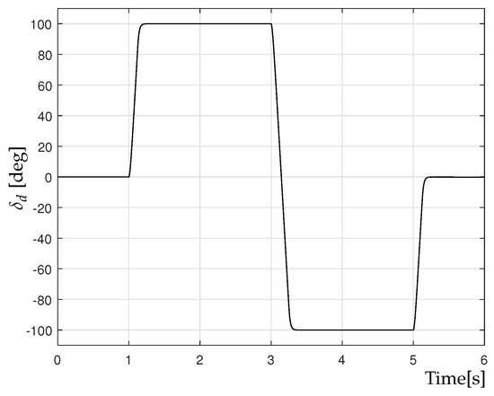
Figure 1. Steering angle ${\delta }_d$.

The initial conditions for the maneuver in the CarSim simulation were set as follows: $v_x\left(0\right)=28$ m/s, $v_y\left(0\right)=0$ m/s, and ${\omega }_z\left(0\right)=0$ rad/s. To introduce a significant challenge for the proposed control system, the longitudinal and lateral tire–road friction coefficients ${\mu }_x$ and ${\mu }_y$ were assumed to undergo an abrupt transition from dry-road conditions ${\mu }_{y,d}=0.9$ to wet-road conditions ${\mu }_{y,w}=0.5$, as illustrated in Figure 2. Furthermore, these friction coefficients were perturbed by white noise, modeled as ${\mu }_x={\mu }_y={\mu }_{y,d}(0.0125\mathcal{R}+1)$ for $t\in [0,3)$ s and ${\mu }_x={\mu }_y={\mu }_{y,w}(0.0125\mathcal{R}+1)$ for $t\ge 3$ s, where $\mathcal{R}$ represents a white noise signal.

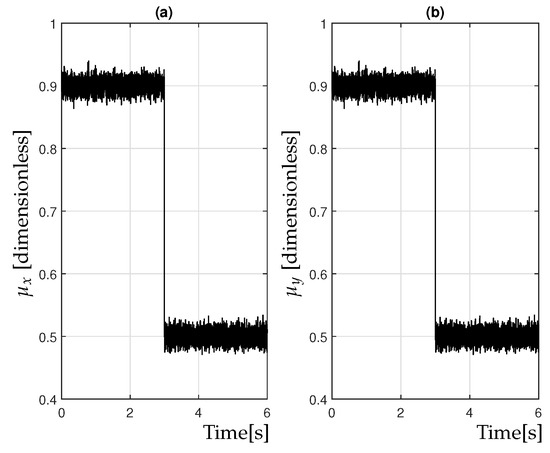
Figure 2. Friction coefficient: (a) ${\mu }_x$; (b) ${\mu }_y$.

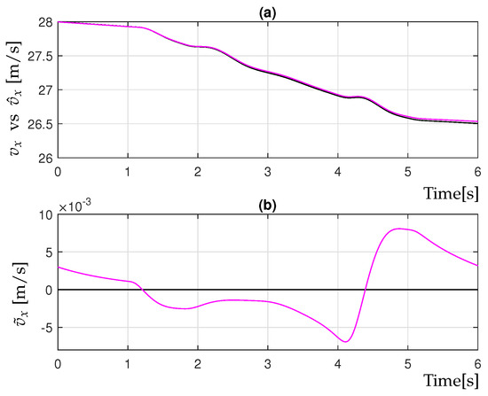
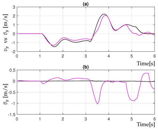
In simulation tests, the adaptive gain HOSM observer designed in (4) was implemented and compared with the nonlinear observer designed in (28). The gains of the observer were set as shown in Table 2. Figure 3a and Figure 4a present the estimate variables ${\widehat{v}}_x$ and ${\widehat{v}}_y$ alongside the actual outputs $v_x$ and $v_y$. As shown in Figure 3a and Figure 4a, the HOSM observer with adaptive gain performs better than the nonlinear observer. This is further supported by Figure 3b and Figure 4b, which show small observer errors.

Table 2. Parameters of the HOSM observer with adaptive gains (4), the nonlinear observer (28), the HOSM controller with adaptive gain (32), and the SM controller (62).

${\mathit{k}}_{\mathit{o},1}$ = 0.1	${\mathit{\omega }}_{\mathit{o},1}$ = 30	${\mathit{\lambda }}_{\mathit{o}}$ = 0.1
$k_{o,2}$ = 0.1	${\omega }_{o,2}$ = 10
$k_{y,1}$ = 1	${\omega }_{y,1}$ = 5	${\lambda }_y$ = 4
$k_{y,2}$ = 1	${\omega }_{y,2}$ = 5
$k_{z,1}$ = 0.12	${\omega }_{z,1}$ = 5.2	${\lambda }_z$ = 5
$k_{z,2}$ = 0.12	${\omega }_{z,2}$ = 5.2
$k_1$ = 90	${\eta }_{s,y}$= 150
$k_2$ = 10	${\eta }_{s,z}$= 150

Figure 3. (a) Longitudinal velocity of the ground vehicle $v_x$ [red] and observer ${\widehat{v}}_x$: HOSM observer with adaptive gains (4) [black] and nonlinear observer (28) [magenta]; (b) observer error ${\tilde{v}}_x=v_x-{\widehat{v}}_x$: HOSM observer with adaptive gains (4) [black] and nonlinear observer (28) [magenta].

Figure 4. (a) Lateral velocity of the ground vehicle $v_y$ [red] and observer ${\widehat{v}}_y$: HOSM observer with adaptive gains (4) [black] and nonlinear observer (28) [magenta]; (b) observer error ${\tilde{v}}_y=v_y-{\widehat{v}}_y$: HOSM observer with adaptive gains (4) [black] and nonlinear observer (28) [magenta].

To support the capabilities of the HOSM observer using adaptive gain in (4), Figure 5 shows the evolution of the adaptive gains ${\gamma }_1\left(t\right)$ and ${\gamma }_2\left(t\right)$.

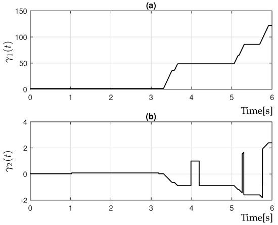
Figure 5. Observer gain: (a) ${\gamma }_1\left(t\right)$; (b) ${\gamma }_2\left(t\right)$.

Furthermore, the proposed HOSM controller using adaptive gain (32) was compared with the controller designed by Sliding Modes (62). In order to have a fair comparison between the proposed controller (32) and SMC (62), the control gains in Table 1 were used. Figure 6a and Figure 7a present the observer variables ${\widehat{v}}_y$ and ${\omega }_z$ along with the references $v_{y,\mathrm{ref}}$ and ${\omega }_{z,\mathrm{ref}}$ to be tracked. Additionally, Figure 6b and Figure 7b depict the tracking errors ${\widehat{v}}_y-v_{y,\mathrm{ref}}$ and ${\omega }_z-{\omega }_{z,\mathrm{ref}}$, respectively. It is possible to notice in Figure 6b and Figure 7b that the proposed controller (32) has a better performance than SMC (62). The parameters considered in the reference model given in (29) are presented in Table 3.

Figure 6. (a) Lateral velocity observer for ground vehicles ${\widehat{v}}_y$ and reference $v_{y,\mathrm{ref}}$ [red]: HOSM controller with adaptive gains (32) [black] and SM controller (62) [magenta]; (b) tracking error $e_y={\widehat{v}}_y-v_{y,\mathrm{ref}}$: HOSM controller with adaptive gains (32) [black] and SM controller (62) [magenta].

Figure 7. (a) Lateral velocity observer for ground vehicles ${\omega }_z$ and reference ${\omega }_{z,\mathrm{ref}}$ [red]: HOSM controller with adaptive gains (32) [black] and SM controller (62) [magenta]; (b) tracking error $e_z={\omega }_z-{\omega }_{z,\mathrm{ref}}$: HOSM controller with adaptive gains (32) [black] and SM controller (62) [magenta].

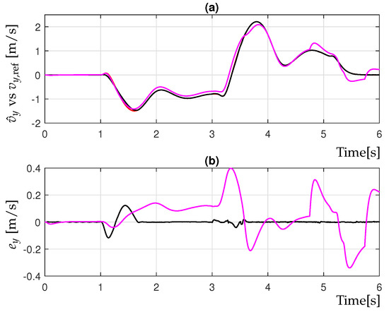
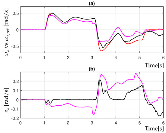
Table 3. Constants of the reference model (29).

${\mathit{m}}_{\mathrm{ref}}=\mathit{m}$	${\mathit{B}}_{\mathit{y},\mathit{f},\mathrm{ref}}={\mathit{B}}_{\mathit{y},\mathit{f}}$	${\mathit{B}}_{\mathit{y},\mathit{r},\mathrm{ref}}=14.7$
$J_{z,\mathrm{ref}}=2488\mathrm{kg}{\mathrm{m}}^2$	$C_{y,f,\mathrm{ref}}=C_{y,f}$	$C_{y,r,\mathrm{ref}}=1.2$
${\mu }_{y,\mathrm{ref}}=0.9$	$D_{y,f,\mathrm{ref}}$ = 10,000 $\mathrm{N}$	$D_{y,r,\mathrm{ref}}$ = 10,000 $\mathrm{N}$

Figure 8 presents the behavior of the active controls, such as ${\Delta }_c$ (due to the AFS input) and yaw moment $M_z$ (due to RTV input),of the scheme proposed in this article (32), demonstrating good tracking between the variables and the reference (see Figure 6 and Figure 7). In addition, Figure 9 and Figure 10 show the behavior of the gains of the ${\Delta }_c$ and $M_z$ control inputs. Moreover, as shown in Figure 8, the proposed controller (32) requires less control effort than the classical SMC (62), resulting in reduced stress in the actuators. Therefore, the proposed controller (32) provides a better general performance with respect to SMC (62).

Figure 8. (a) AFS Input ${\Delta }_f$; (b) RTV Input $M_z$: HOSM controller with adaptive gains (32) [black] and SM controller (62) [magenta].

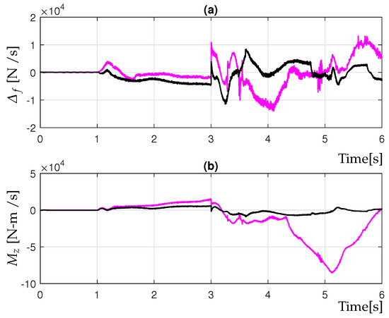
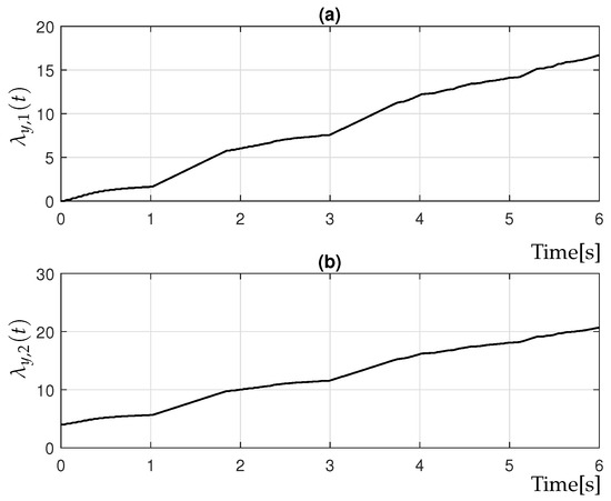
Figure 9. Controller gain: (a) ${\lambda }_{y,1}\left(t\right)$; (b) ${\lambda }_{y,2}\left(t\right)$.

Figure 10. Controller gain: (a) ${\lambda }_{z,1}\left(t\right)$; (b) ${\lambda }_{z,2}\left(t\right)$.

The external disturbances affecting the vehicle are primarily caused by wind (refer to Figure 11), resulting in longitudinal and lateral forces $F_{d,x}$ and $F_{d,y}$, and a yaw moment $M_{d,z}$. The forces and yaw moment generated by wind are expressed as $F_{d,x}=-A_{s,f}\rho c_{a,x}{v}_{aw,x}^2/2$ and $F_{d,y}=-A_{s,l}\rho c_{a,y}{v}_{aw,y}^2/2$, where $A_{s,f}=2.59 {\mathrm{m}}^2$ and $A_{s,l}=5.1{\mathrm{m}}^2$ represent the frontal and lateral projected areas of the vehicle, $\rho$ is the air density, and $c_{a,x}=0.28$ and $c_{a,y}=0.54$ are the aerodynamic coefficients (dimensionless) for the front and lateral surfaces, respectively. The wind velocity components are given by $v_{w,x}=v_{w,X}cos{\alpha }_z+v_{w,Y}sin{\alpha }_z$ and $v_{w,y}=-v_{w,X}sin{\alpha }_z+v_{w,Y}cos{\alpha }_z$. The apparent wind velocity components are expressed as $v_{aw,x}=v_x-v_{w,x}$ and $v_{aw,y}=v_y-v_{w,y}$.

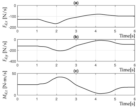
Figure 11. Disturbances: (a) $F_{d,x}$; (b) $F_{d,y}$; (c) $M_{d,z}$.

To support the capabilities of the HOSM controller with adaptive gain proposed in (32), Figure 9 and Figure 10 show the evolution of the adaptive gains ${\Delta }_c$ and $M_z$ in the HOSM controller integrated into the control law (32).

6. Conclusions

This study presents the development and evaluation of a dynamic HOSM controller with adaptive gains designed for ground vehicles utilizing Active Front Steering (AFS) and Rear Torque Vectoring (RTV) systems. A key contribution of this work is the integration of a nonlinear observer with adaptive gains for estimating lateral velocity, paired with an estimator capable of reconstructing parametric uncertainties and external disturbances within a finite time. These features are pivotal for enhancing trajectory control under challenging driving conditions and dynamic variations in the vehicle’s behavior. The simulation results obtained using CarSim validate the controller’s effectiveness in achieving accurate trajectory tracking, even in the presence of significant parametric variations and external perturbations, such as wind gusts. Overall, this research advances robust vehicle control by proposing a nonlinear control approach with adaptive gain that ensures high-precision disturbance estimation and adaptation to system variations. While the simulation findings are encouraging, future work will extend the proposed adaptive HOSM observer–controller framework to address additional challenges such as sensitivity to sensor noise and split-road conditions. For the former, Physics-Informed Neural Networks (PINNs) will be investigated for real-time noise filtering and state reconstruction, enhancing estimation accuracy and control robustness under noisy measurements. For the latter, asymmetric traction scenarios—where one side of the vehicle operates on a low-friction surface and the other on high-friction pavement—will be considered to evaluate stability and control performance under extreme conditions. Furthermore, hardware-in-the-loop (HIL) implementations on embedded platforms such as the NVIDIA Jetson Orin NX or Jetson Nano will be pursued, integrating both the high-fidelity vehicle model and the control algorithm to assess real-time feasibility and readiness for deployment in physical vehicles.

References

- Shtessel, Y.; Edwards, C.; Fridman, L.; Levant, A. Sliding Mode Control and Observation; Springer: New York, NY, USA, 2014. [Google Scholar]
- Acosta-Lúa, C.; Castillo-Toledo, B.; Cespi, R.; Di Gennaro, S. An integrated active nonlinear controller for wheeled vehicles. J. Frankl. Inst. 2015, 352, 4890–4910. [Google Scholar] [CrossRef]
- Acosta-Lúa, C.; Di Gennaro, S. Nonlinear adaptive tracking for ground vehicles in the presence of lateral wind disturbance and parameter variations. J. Frankl. Inst. 2017, 354, 2742–2768. [Google Scholar] [CrossRef]
- Acosta-Lúa, C.; Bianchi, D.; Di Gennaro, S. Nonlinear observer-based adaptive control of ground vehicles with uncertainty estimation. J. Frankl. Inst. 2023, 360, 14175–14189. [Google Scholar] [CrossRef]
- Borri, A.; Bianchi, D.; Di Benedetto, M.D.; Di Gennaro, S. Optimal workload actuator balancing and dynamic reference generation in active vehicle control. J. Frankl. Inst. 2017, 354, 1722–1740. [Google Scholar] [CrossRef]
- Mirzaei, M.; Mirzaeinejad, H. Fuzzy scheduled optimal control of integrated vehicle braking and steering systems. IEEE/ASME Trans. Mechatronics 2017, 22, 2369–2379. [Google Scholar] [CrossRef]
- Navarrete-Guzmán, A.; Di Gennaro, S.; Rivera Domínguez, J.; Acosta Lua, C.; Loukianov, A.G.; Castillo-Toledo, B. Enhanced discrete–time modeling via variational integrators and digital controller design for ground vehicles. IEEE Trans. Ind. Electron. 2016, 63, 6375–6385. [Google Scholar] [CrossRef]
- Sun, Z.; Zheng, J.; Man, Z.; Wang, H.; Lu, R. Sliding mode–based active disturbance rejection control for vehicle steer–by–wire systems. IET Cyber-Phys. Syst. Theory Appl. 2018, 3, 1–10. [Google Scholar] [CrossRef]
- Guo, H.; Liu, F.; Xu, F.; Chen, H.; Cao, D.; Ji, Y. Nonlinear model predictive lateral stability control of active chassis for intelligent vehicles and its FPGA implementation. IEEE Trans. Syst. Man Cybern. Syst. 2019, 49, 2–13. [Google Scholar] [CrossRef]
- Acosta-Lúa, C.; Di Gennaro, S.; Navarrete-Guzman, A.; Ortega Cisneros, S.; Rivera Domínguez, J. Digital implementation via FPGA of controllers for active control of ground vehicles. IEEE Trans. Ind. Inform. 2019, 5, 2253–2264. [Google Scholar]
- Etienne, L.; Acosta-Lúa, C.; Di Gennaro, S.; Barbot, J.P. A super-twisting controller for active control of ground vehicles with lateral tire-road friction estimation and CarSim validation. Int. J. Control. Autom. Syst. 2020, 18, 1177–1189. [Google Scholar] [CrossRef]
- Yu, J.; Liu, Z.; Shi, P. Robust State-Estimator-Based Control of Uncertain Semi-Markovian Jump Systems Subject to Actuator Failures and Time-Varying Delay. IEEE Trans. Autom. Control 2024, 69, 487–494. [Google Scholar] [CrossRef]
- Bianchi, D.; Borri, A.; Benedetto, M.D.; Di Gennaro, S. Active attitude control of ground vehicles with partially unknown model. IFAC-PapersOnLine 2020, 53, 14621–14626. [Google Scholar] [CrossRef]
- Liu, W.; He, C.; Ji, Y.; Hou, X.; Zhang, J. Active disturbance rejection control of path following control for autonomous ground vehicles. In Proceedings of the 2020 Chinese Automation Congress, Shanghai, China, 6–8 November 2020; pp. 6839–6844. [Google Scholar]
- Swain, S.K.; Rath, J.J.; Veluvolu, K.C. Neural Network Based Robust Lateral Control for an Autonomous Vehicle. Electronics 2021, 10, 510. [Google Scholar] [CrossRef]
- Emelyanov, S.V.; Korovin, S.K.; Levantovsky, L.V. Higher Order Sliding Regimes in the Binary Control Systems. Dokl. Akad. Nauk. Russian Acad. Sci. 1986, 287, 1338–1342. [Google Scholar]
- Utkin, V. Discussion aspects of high–order sliding mode control. IEEE Trans. Autom. Control 2015, 61, 829–833. [Google Scholar] [CrossRef]
- Utkin, V.; Pozniak, A.; Orlov, Y.; Polyakov, A. Conventional and High Order Sliding Mode Control. J. Frankl. Inst. 2020, 35, 10244–10261. [Google Scholar] [CrossRef]
- Mercado-Uribe, J.A.; Moreno, J.A. Discontinuous integral action for arbitrary relative degree in sliding–mode control. Automatica 2020, 118, 109018. [Google Scholar] [CrossRef]
- Fridman, L.; Moreno, J.; Iriarte, R. Sliding Modes After the First Decade of the 21st Century: State of the Art; Lecture Notes in Control and Information Sciences; Springer Verlag: Berlin/Heidelberg, Germany, 2011. [Google Scholar]
- Kreerenko, O.D. Nonlinear Adaptive Control of UAV Flight Under the Influence of Wind Disturbance. In Proceedings of the 2024 IEEE International Russian Smart Industry Conference (SmartIndustryCon), Sochi, Russia, 25–29 March 2024; pp. 813–818. [Google Scholar]
- Imran, I.H.; Wood, K.; Montazeri, A. Adaptive Control of Unmanned Aerial Vehicles with Varying Payload and Full Parametric Uncertainties. Electronics 2024, 13, 347–358. [Google Scholar] [CrossRef]
- Yoon, D.S.; Choi, S.B. Adaptive Control for Suspension System of In-Wheel Motor Vehicle with Magnetorheological Damper. Machines 2024, 12, 433–443. [Google Scholar] [CrossRef]
- He, S.; Xu, X.; Xie, J.; Wang, F.; Liu, Z. Adaptive control of dual-motor autonomous steering system for intelligent vehicles via Bi-LSTM and fuzzy methods. Control Eng. Pract. 2023, 130, 105362. [Google Scholar] [CrossRef]
- Setlur, P.; Wagner, J.R.; Dawson, D.M.; Braganza, D. A trajectory tracking steer-by-wire control system for ground vehicles. IEEE Trans. Veh. Technol. 2006, 55, 76–85. [Google Scholar] [CrossRef]
- Burgio, G.; Zeglaar, P. Integrated Vehicle Control using Steering and Brakes. Int. J. Control 2006, 79, 162–169. [Google Scholar] [CrossRef]
- Pacejka, H. Tyre and Vehicle Dynamics; Elsevier: Amsterdam, The Netherlands, 2006. [Google Scholar]
Disclaimer/Publisher’s Note: The statements, opinions and data contained in all publications are solely those of the individual author(s) and contributor(s) and not of MDPI and/or the editor(s). MDPI and/or the editor(s) disclaim responsibility for any injury to people or property resulting from any ideas, methods, instructions or products referred to in the content. |
© 2025 by the authors. Licensee MDPI, Basel, Switzerland. This article is an open access article distributed under the terms and conditions of the Creative Commons Attribution (CC BY) license (https://creativecommons.org/licenses/by/4.0/).