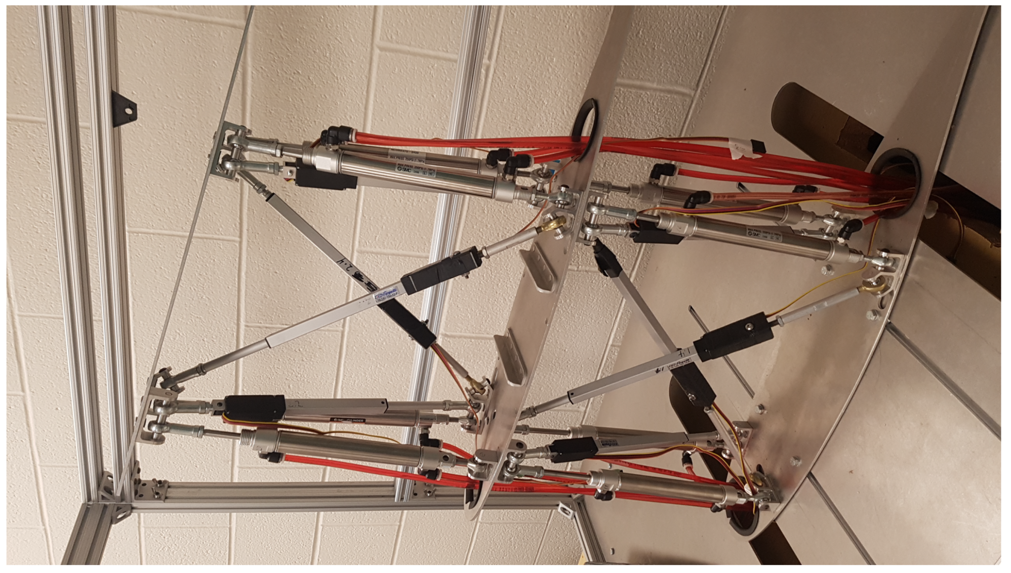
Figure 1.
Reconfigurable modular morphing wing, view 1.
Figure 1.
Reconfigurable modular morphing wing, view 1.
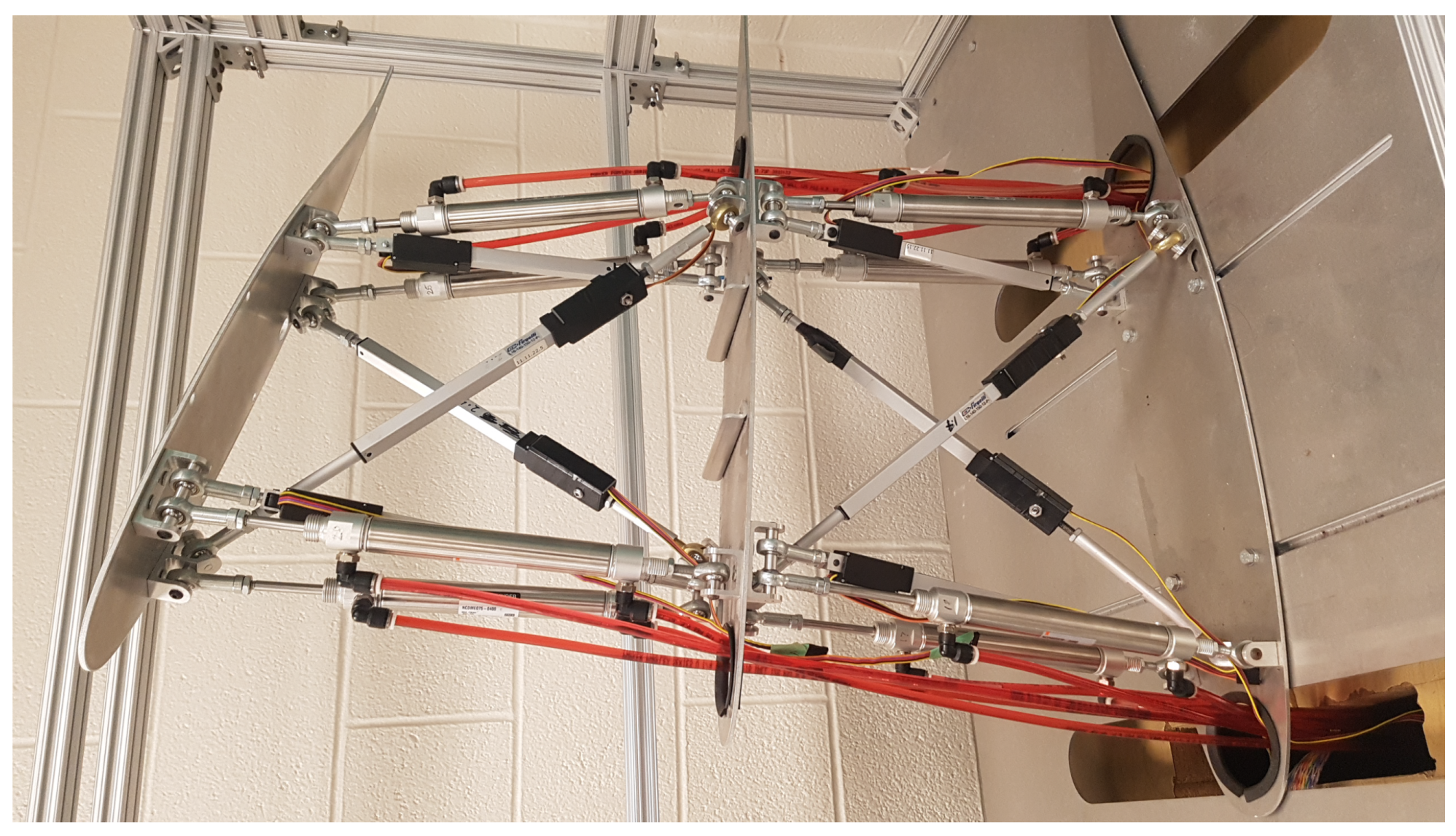
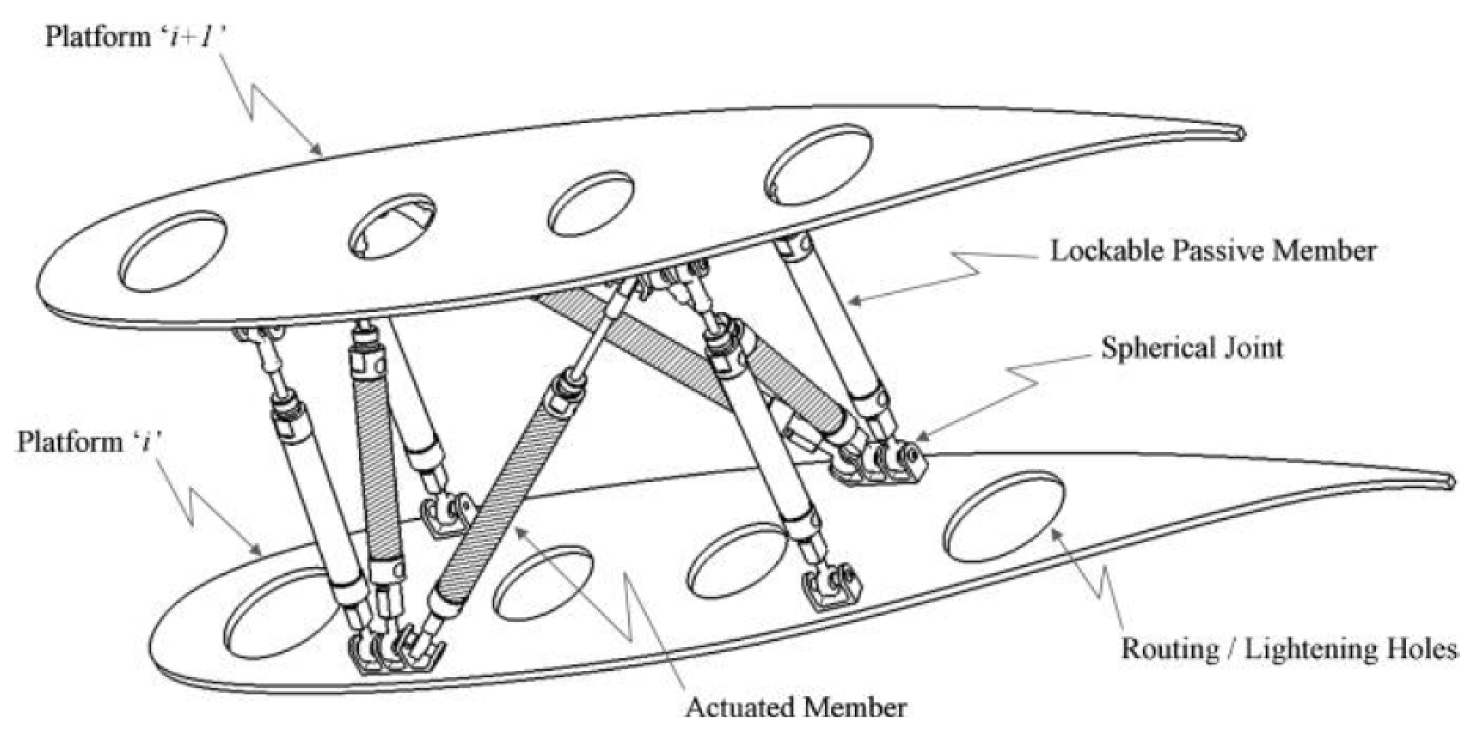
Figure 2.
Reconfigurable modular morphing wing, view 2.
Figure 2.
Reconfigurable modular morphing wing, view 2.
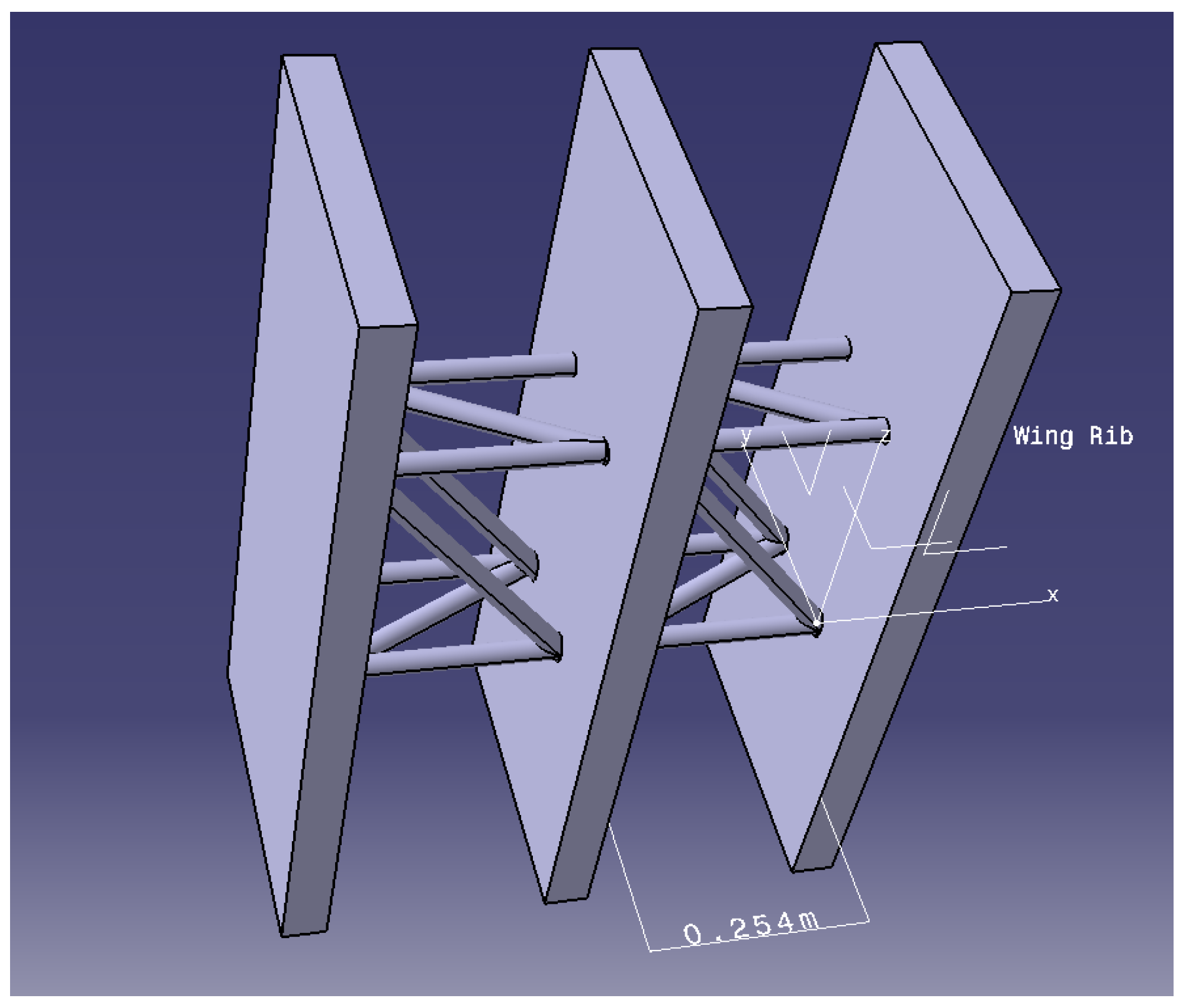
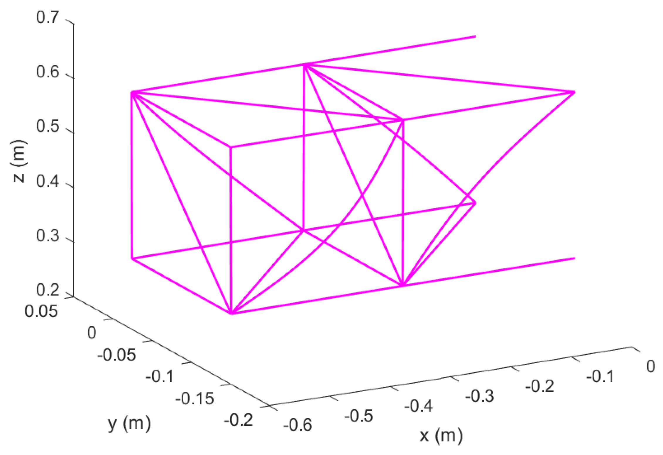
Figure 3.
Configuration of structural element connections in morphing Wing, Topology 1.
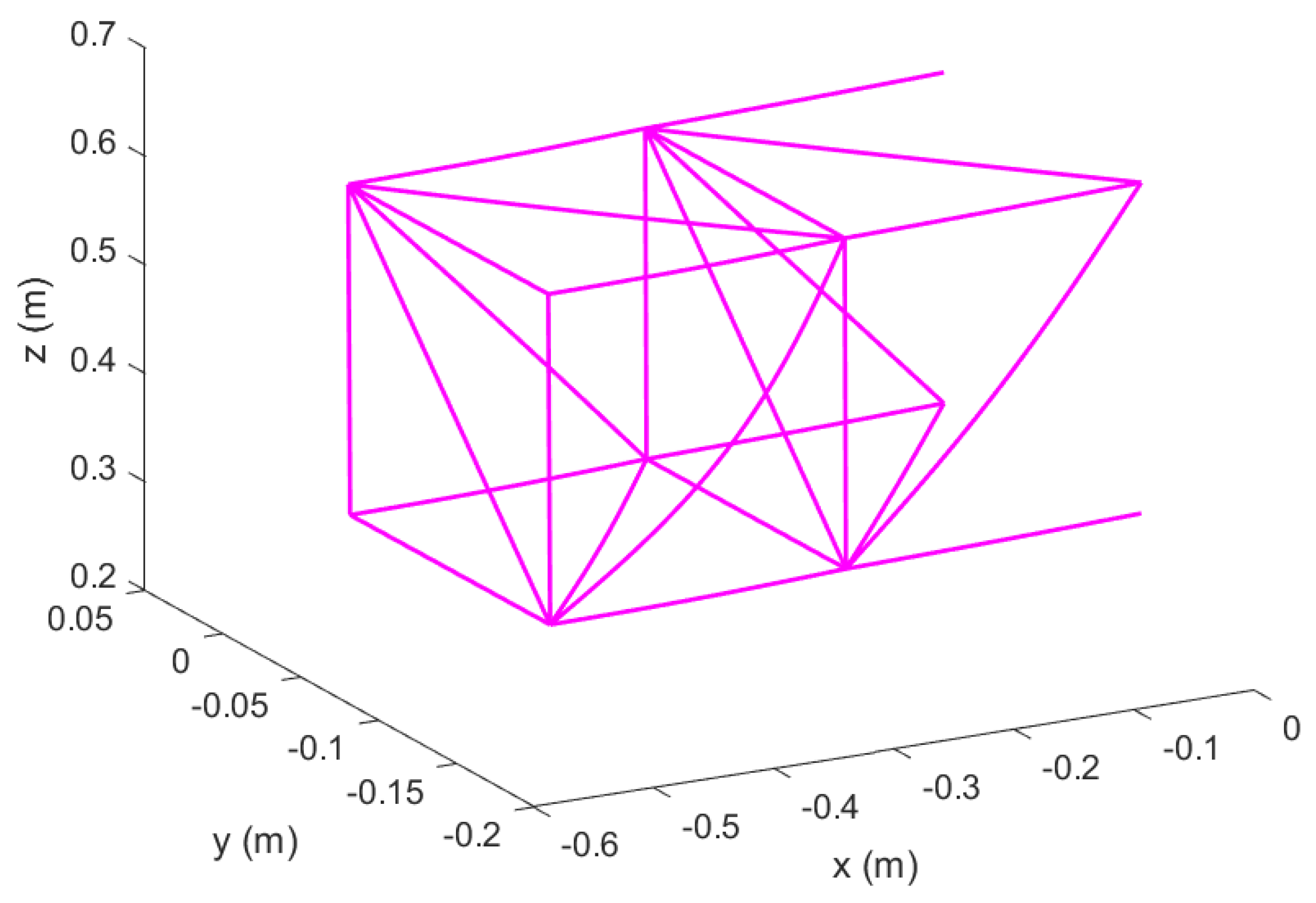
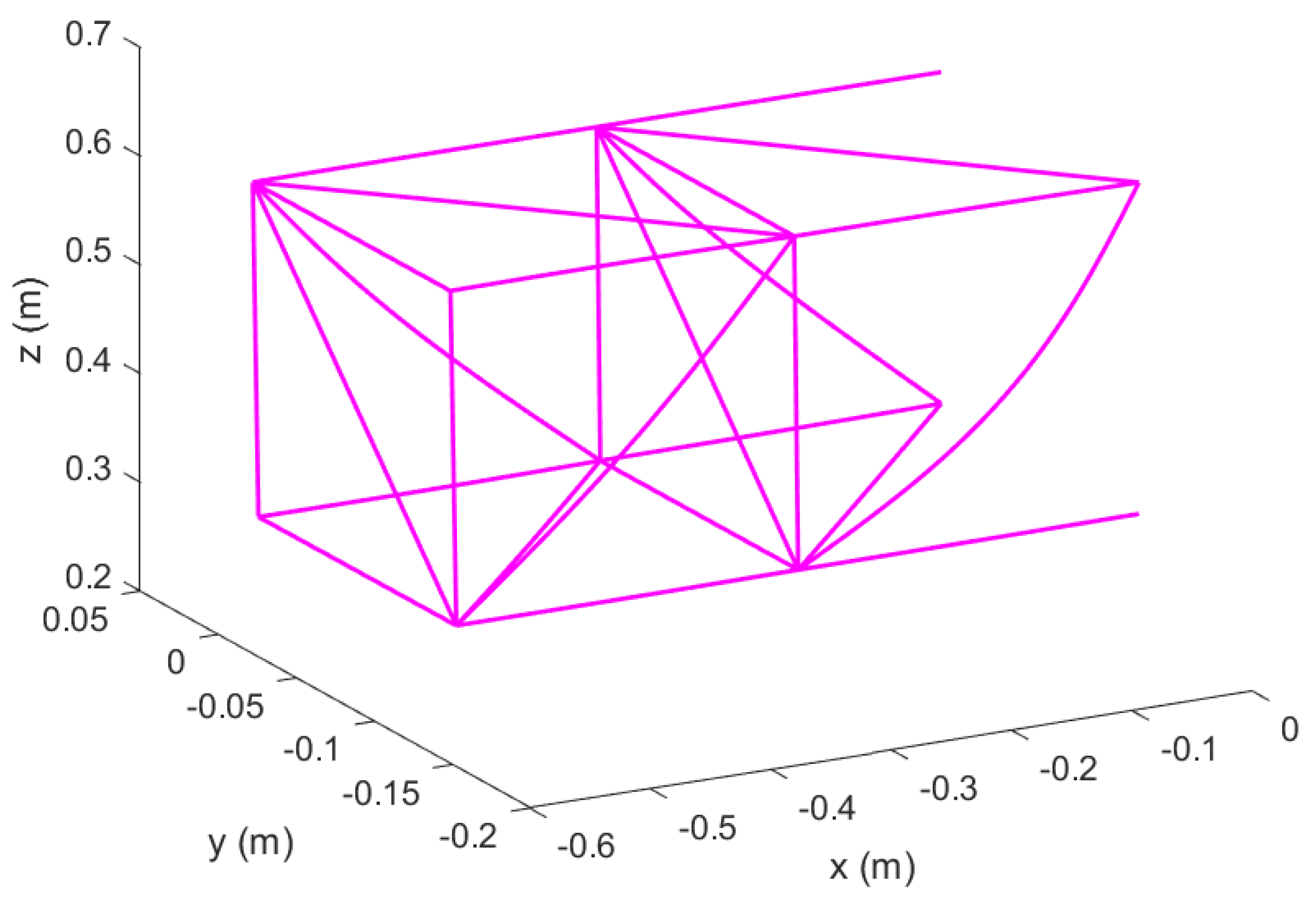
Figure 3.
Configuration of structural element connections in morphing Wing, Topology 1.
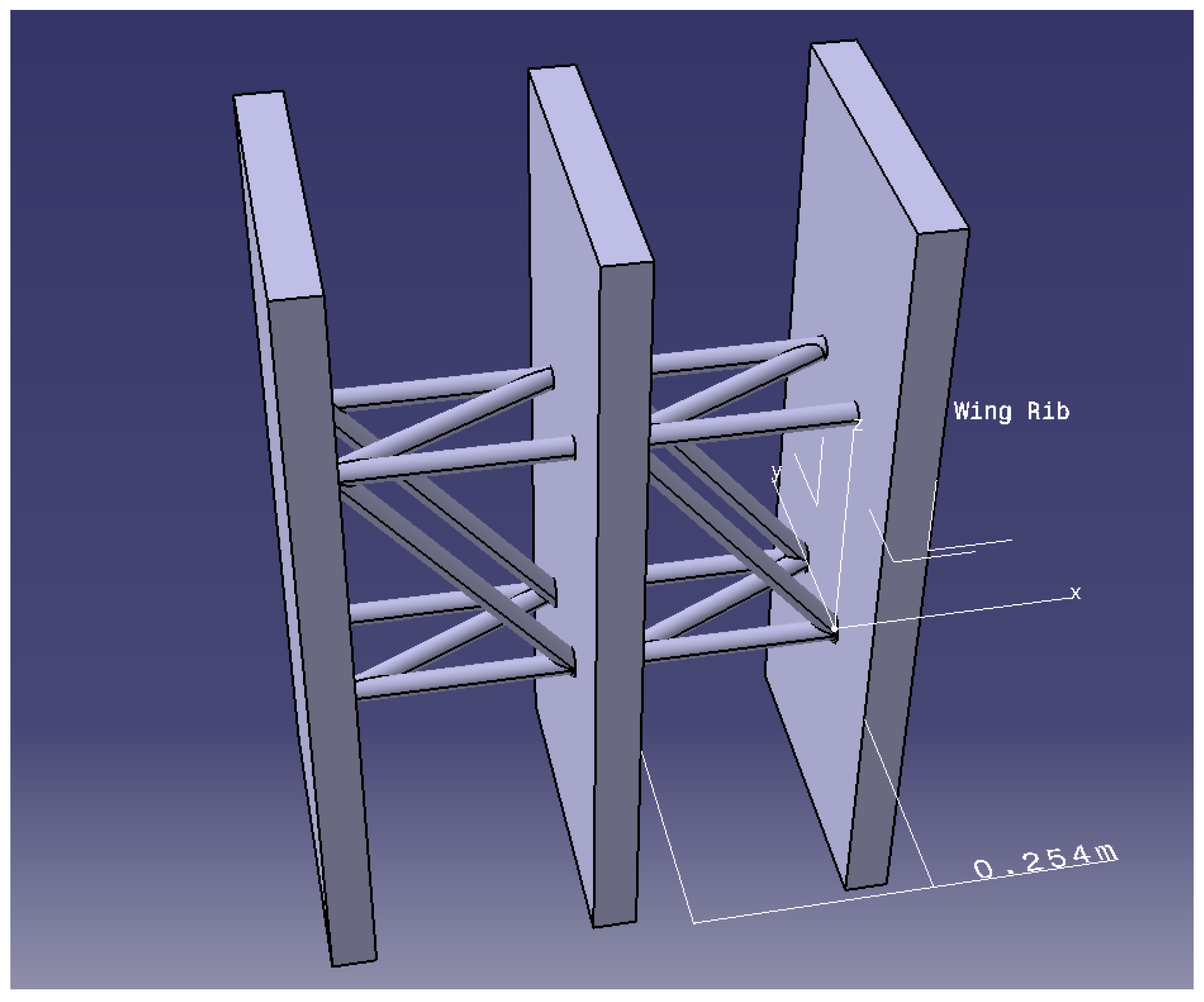
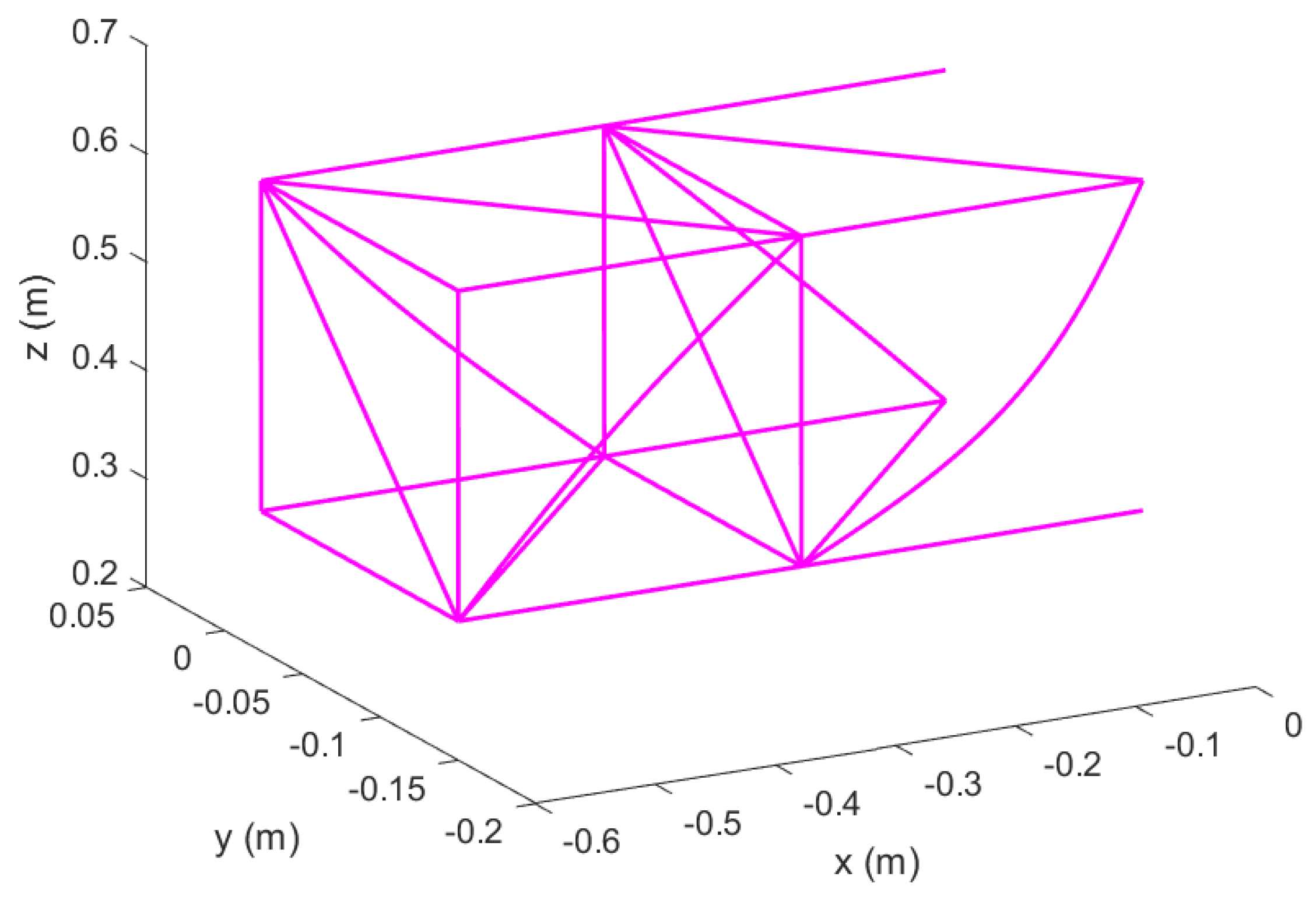
Figure 4.
Configuration of structural element connections in morphing wing, Topology 2.
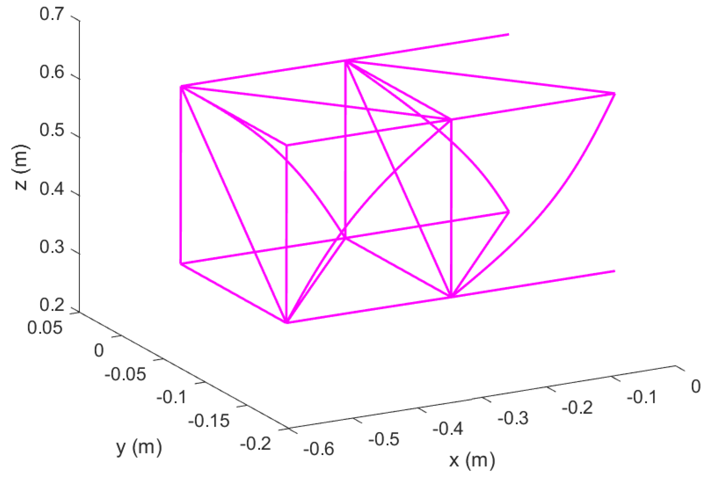
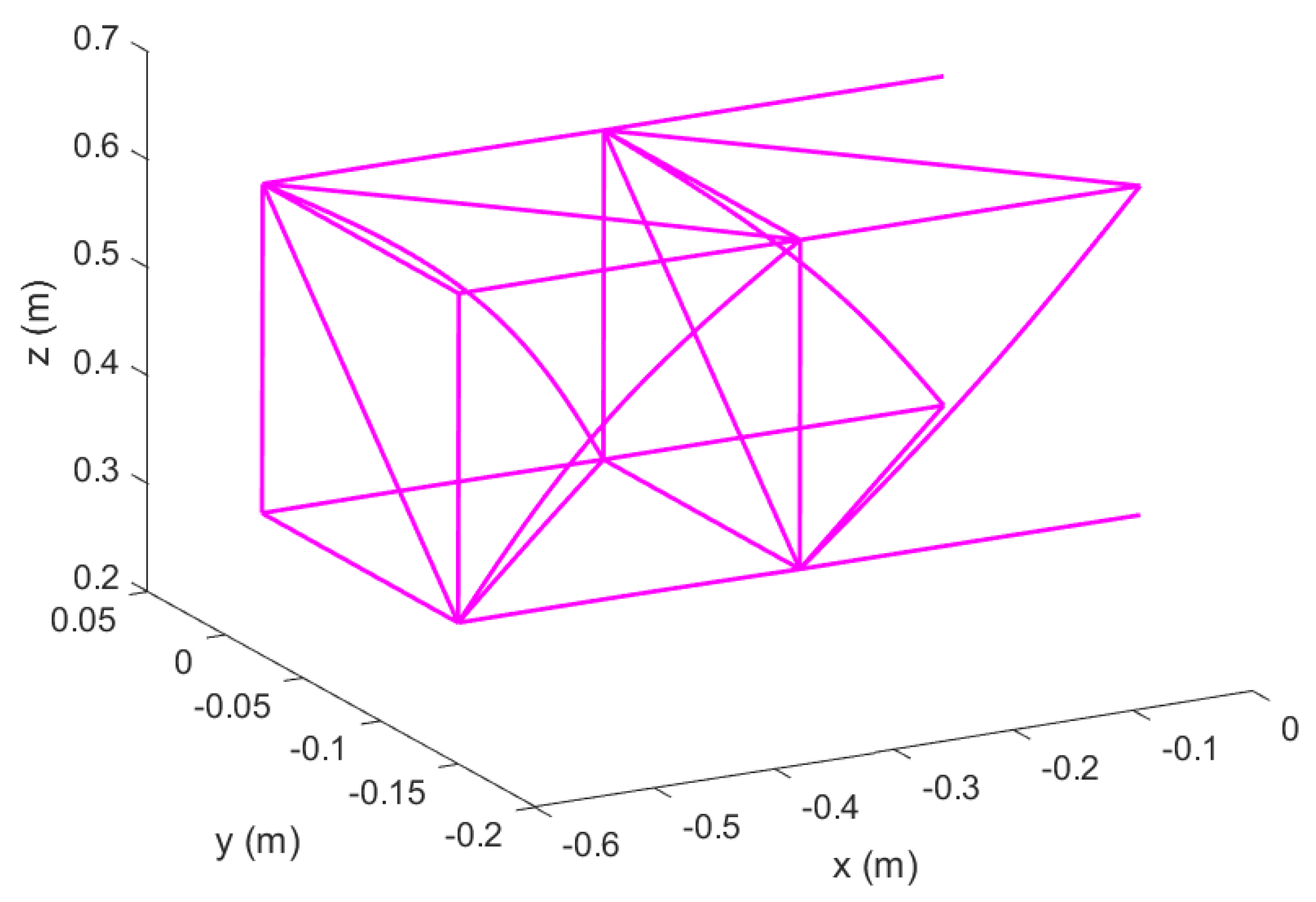
Figure 4.
Configuration of structural element connections in morphing wing, Topology 2.
Figure 5.
Mechanism of the reconfigurable morphing wing, Topology 1 [
6].
Figure 5.
Mechanism of the reconfigurable morphing wing, Topology 1 [
6].
Figure 6.
Mode 1 (out–of–plane/flapping) of two Euler–Bernoulli Beams connected through hinged joint.
Figure 6.
Mode 1 (out–of–plane/flapping) of two Euler–Bernoulli Beams connected through hinged joint.
Figure 7.
Mode 2 (in–plane/lead–lag) of two Euler–Bernoulli Beams connected through hinged joint.
Figure 7.
Mode 2 (in–plane/lead–lag) of two Euler–Bernoulli Beams connected through hinged joint.
Figure 8.
Mode 3 (out–of–plane/flapping) of two Euler–Bernoulli Beams connected through hinged joint.
Figure 8.
Mode 3 (out–of–plane/flapping) of two Euler–Bernoulli Beams connected through hinged joint.
Figure 9.
Mode 4 (in–plane/lead–lag) of two Euler–Bernoulli Beams connected through hinged joint.
Figure 9.
Mode 4 (in–plane/lead–lag) of two Euler–Bernoulli Beams connected through hinged joint.
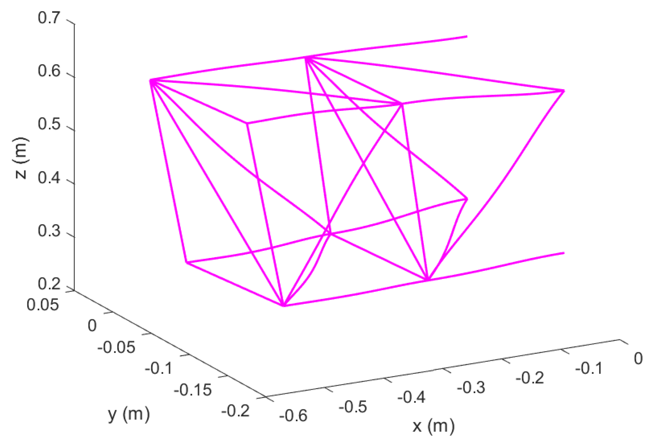
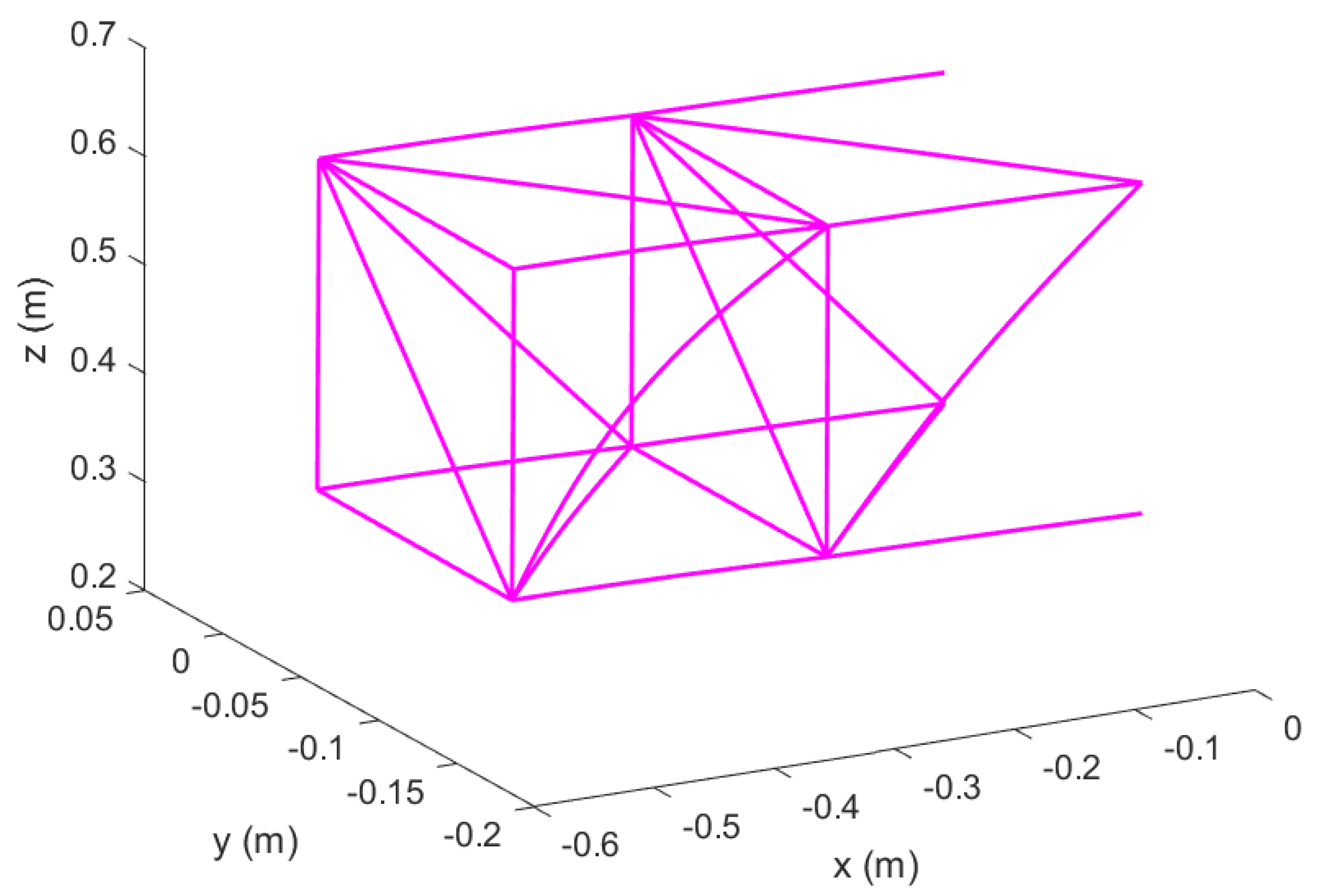
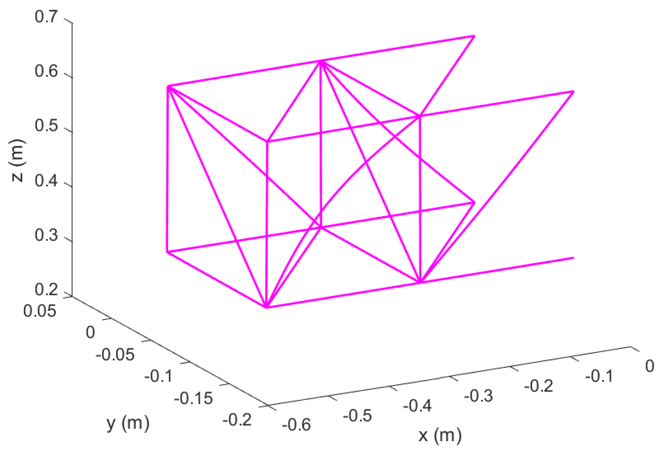
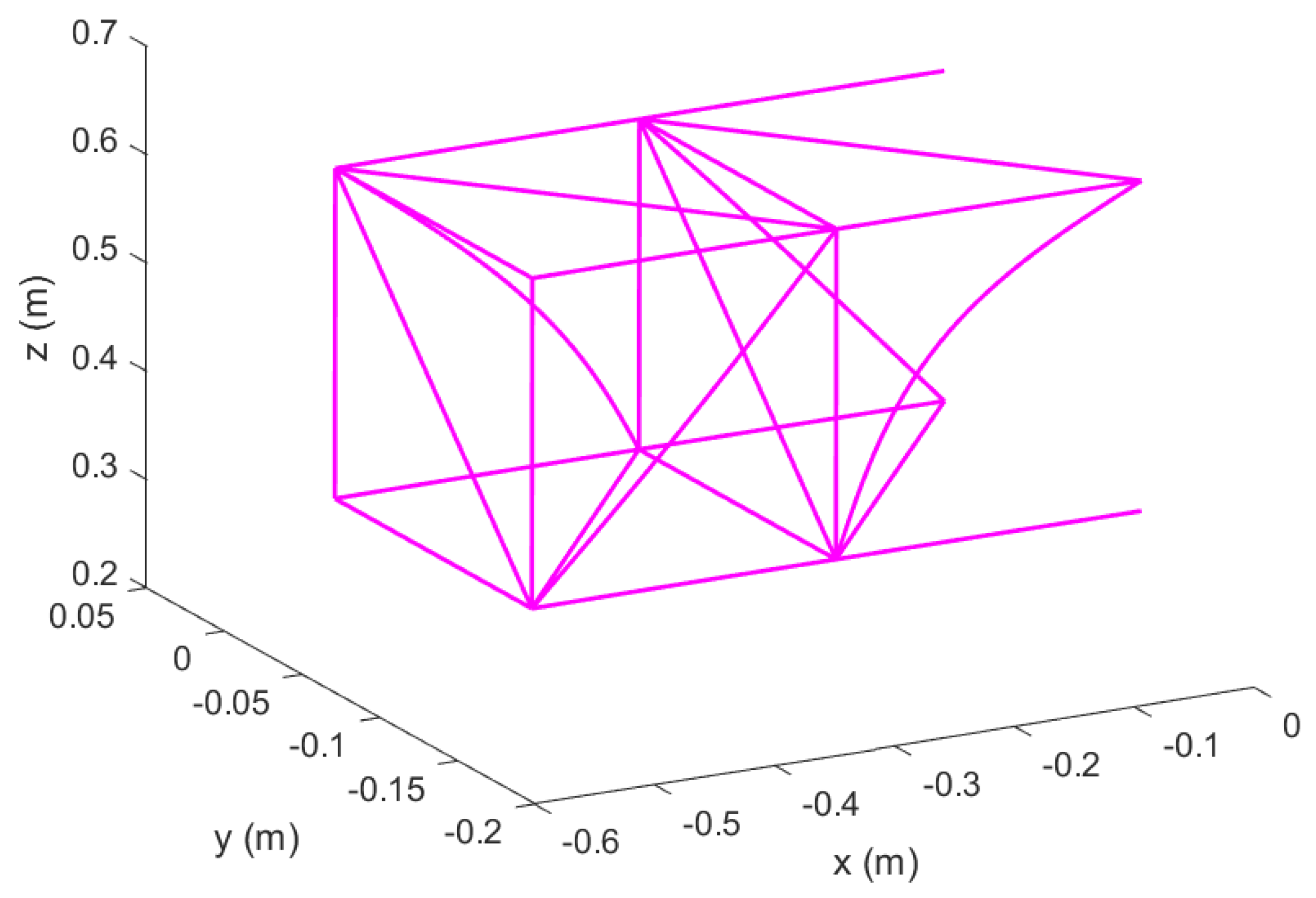
Figure 10.
Un–morphed wing in Topology 1 with no hinged ends; original configuration.
Figure 10.
Un–morphed wing in Topology 1 with no hinged ends; original configuration.
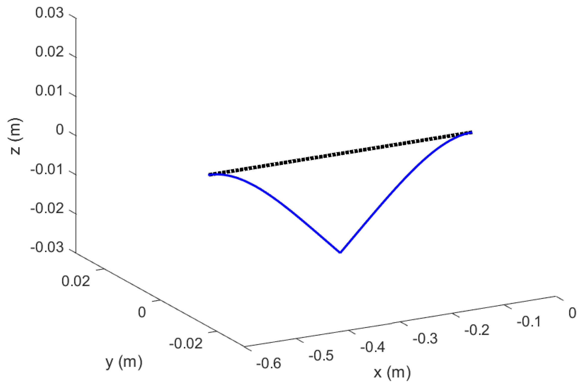
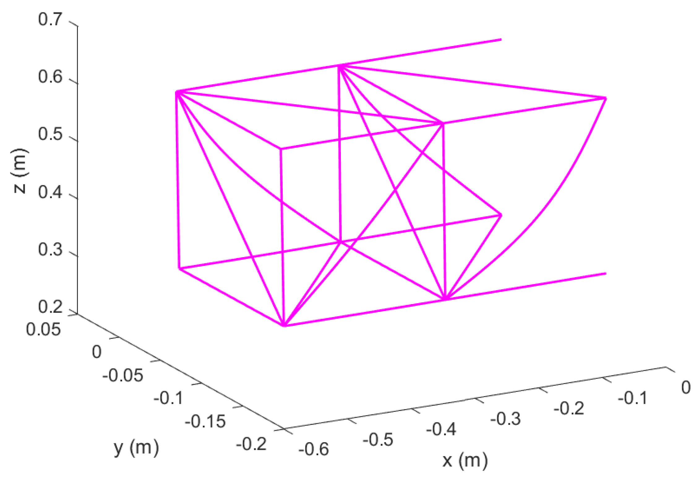
Figure 11.
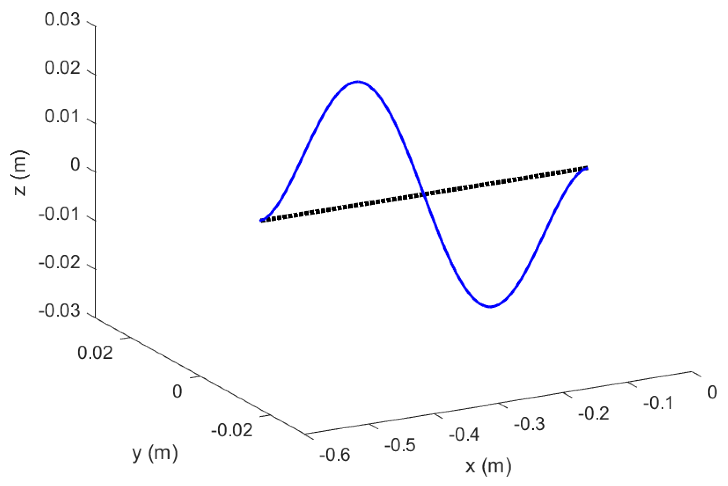
Mode 1 of Euler–Bernoulli Beams in Topology 1 with no hinged ends; original configuration.
Figure 11.
Mode 1 of Euler–Bernoulli Beams in Topology 1 with no hinged ends; original configuration.
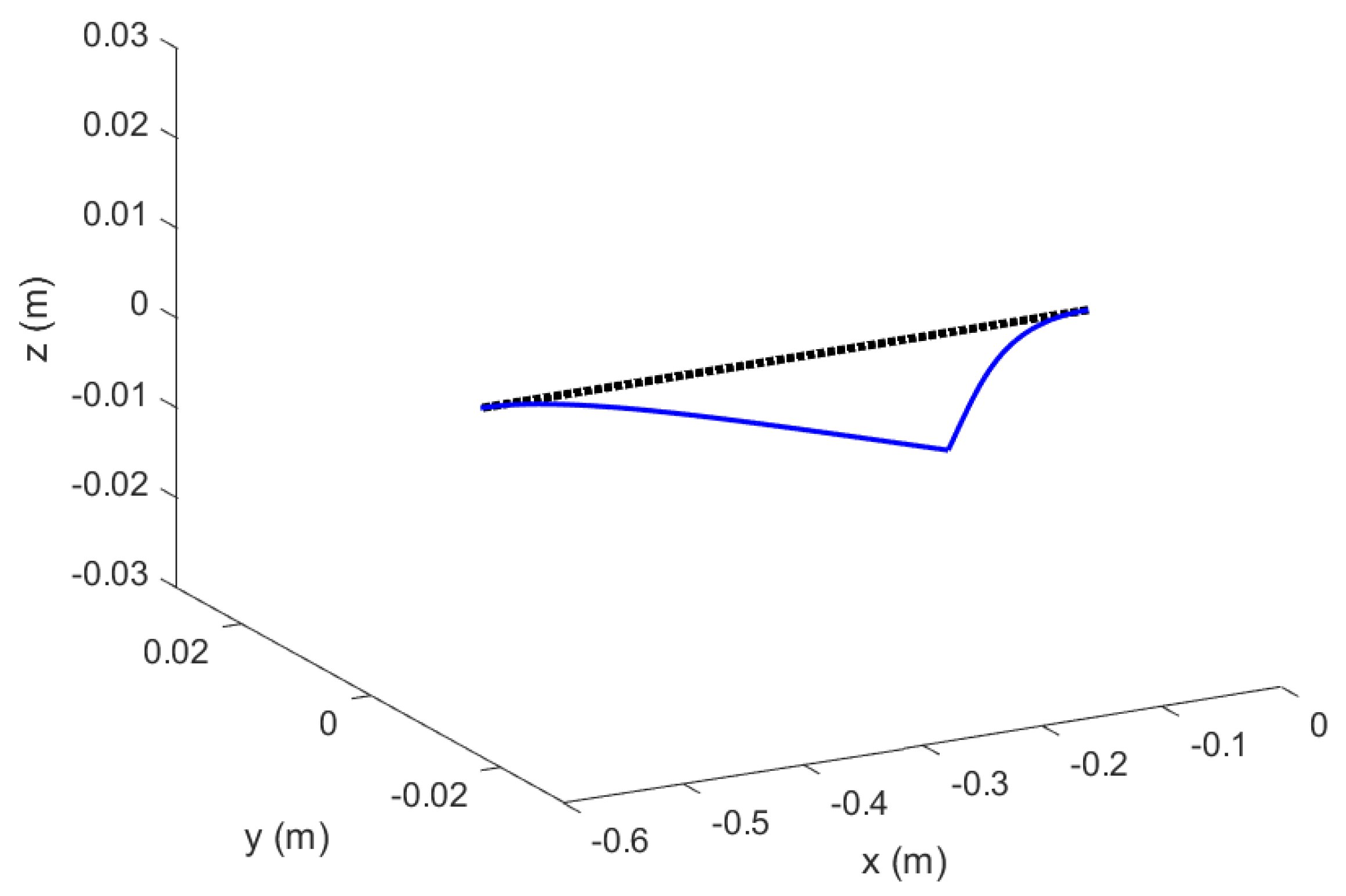
Figure 12.
Mode 2 of Euler–Bernoulli Beams in Topology 1 with no hinged ends; original configuration.
Figure 12.
Mode 2 of Euler–Bernoulli Beams in Topology 1 with no hinged ends; original configuration.
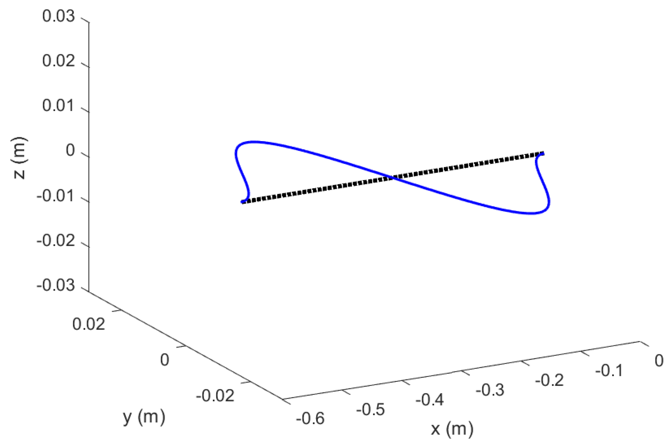
Figure 13.
Mode 3 of Euler–Bernoulli Beams in Topology 1 with no hinged ends; original configuration.
Figure 13.
Mode 3 of Euler–Bernoulli Beams in Topology 1 with no hinged ends; original configuration.
Figure 14.
Mode 4 of Euler–Bernoulli Beams in Topology 1 with no hinged ends; original configuration.
Figure 14.
Mode 4 of Euler–Bernoulli Beams in Topology 1 with no hinged ends; original configuration.
Figure 15.
Mode 5 of Euler–Bernoulli Beams in Topology 1 with no hinged ends; original configuration.
Figure 15.
Mode 5 of Euler–Bernoulli Beams in Topology 1 with no hinged ends; original configuration.
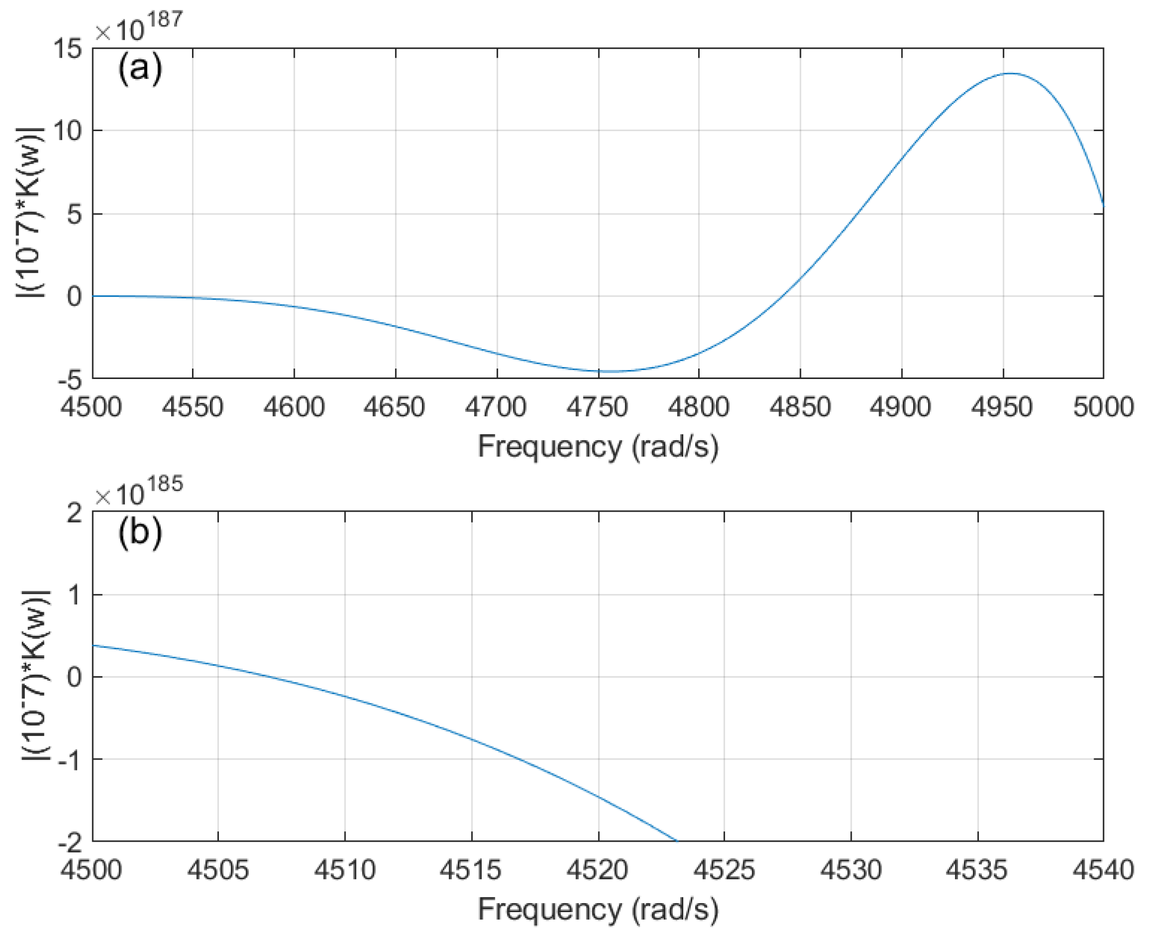
Figure 16.
Dynamic Stiffness Matrix plot of Euler–Bernoulli Beams in Topology 1 with unhinged ends using DSM; original configuration (a) a selected region of natural frequencies showing zero–crossing at the 10th natural frequency (b) a detailed section showing zero–crossing at the 9th natural frequency.
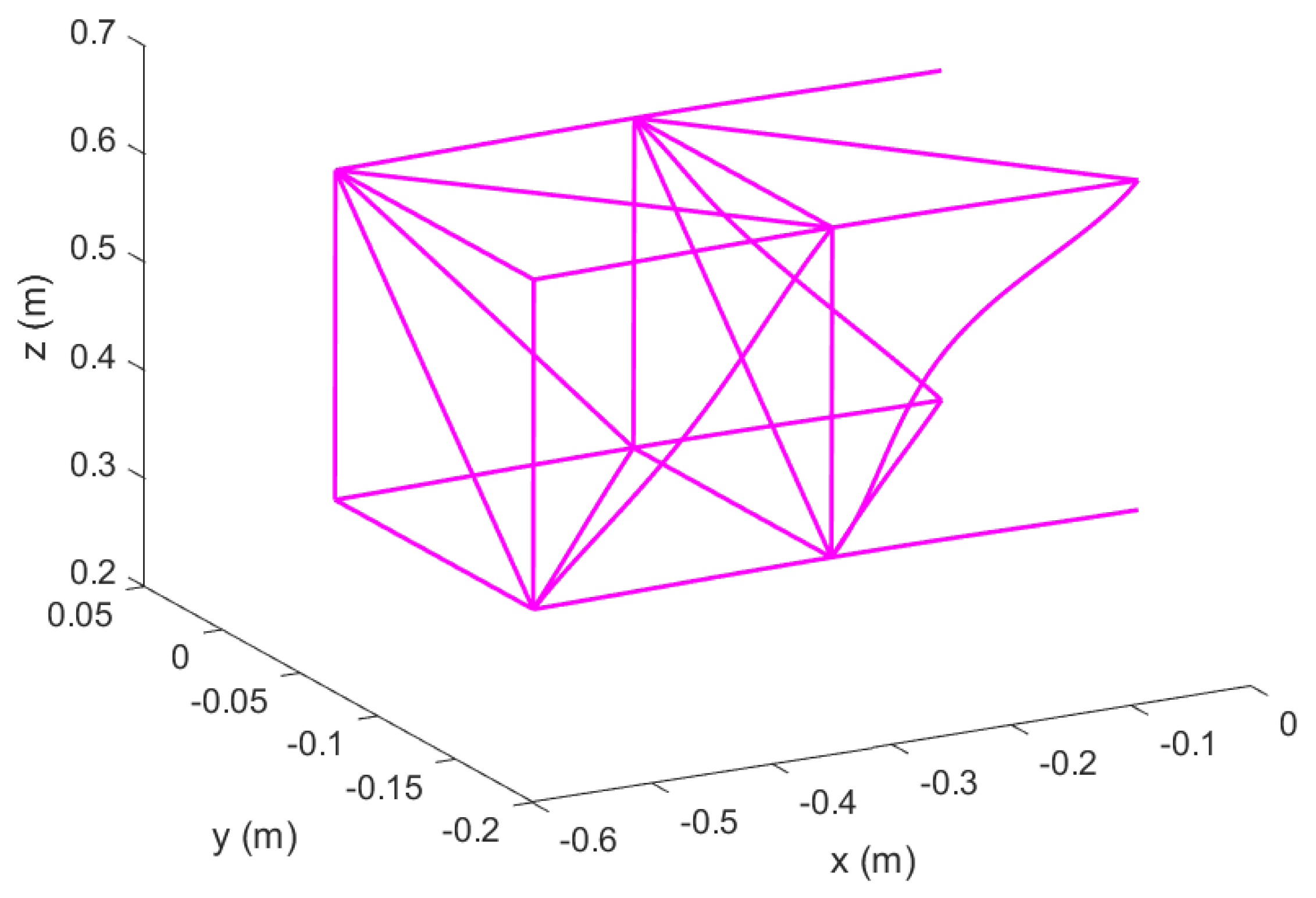
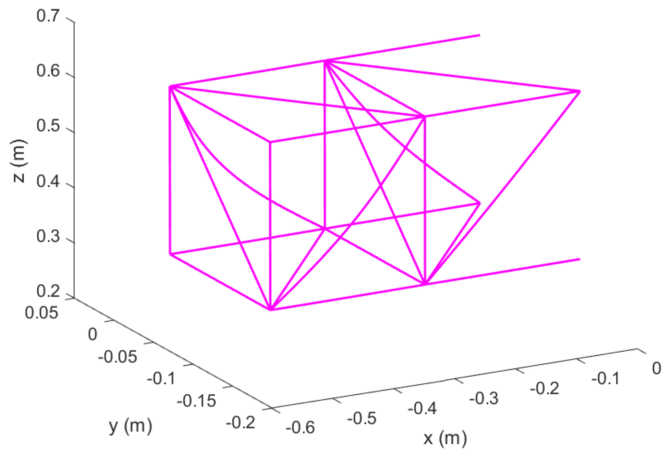
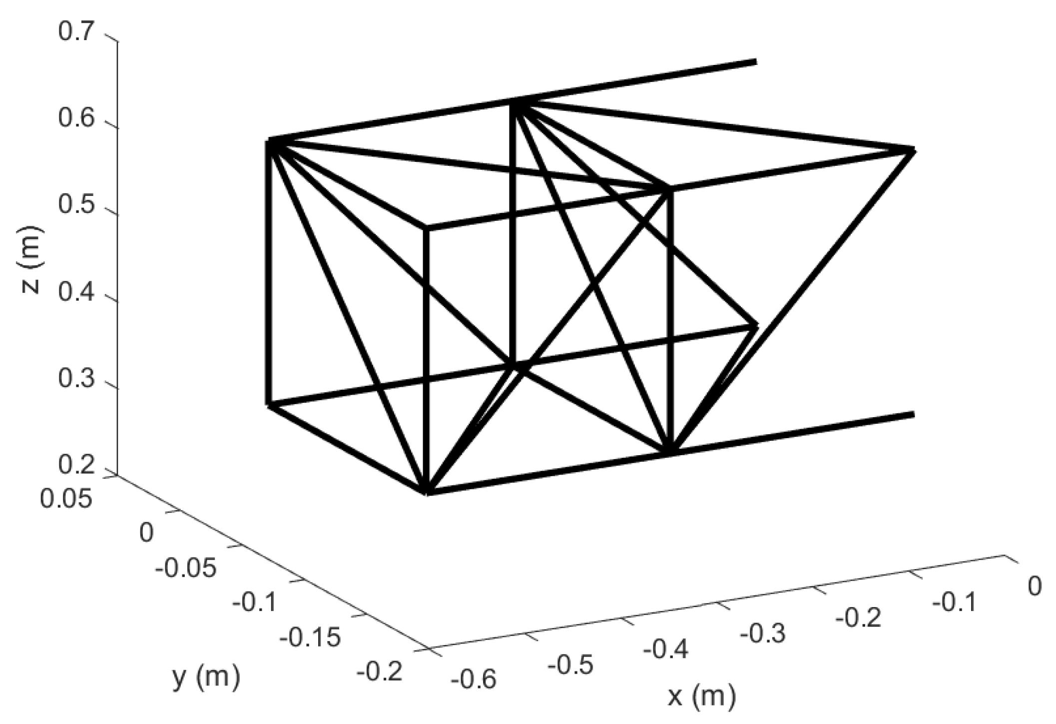
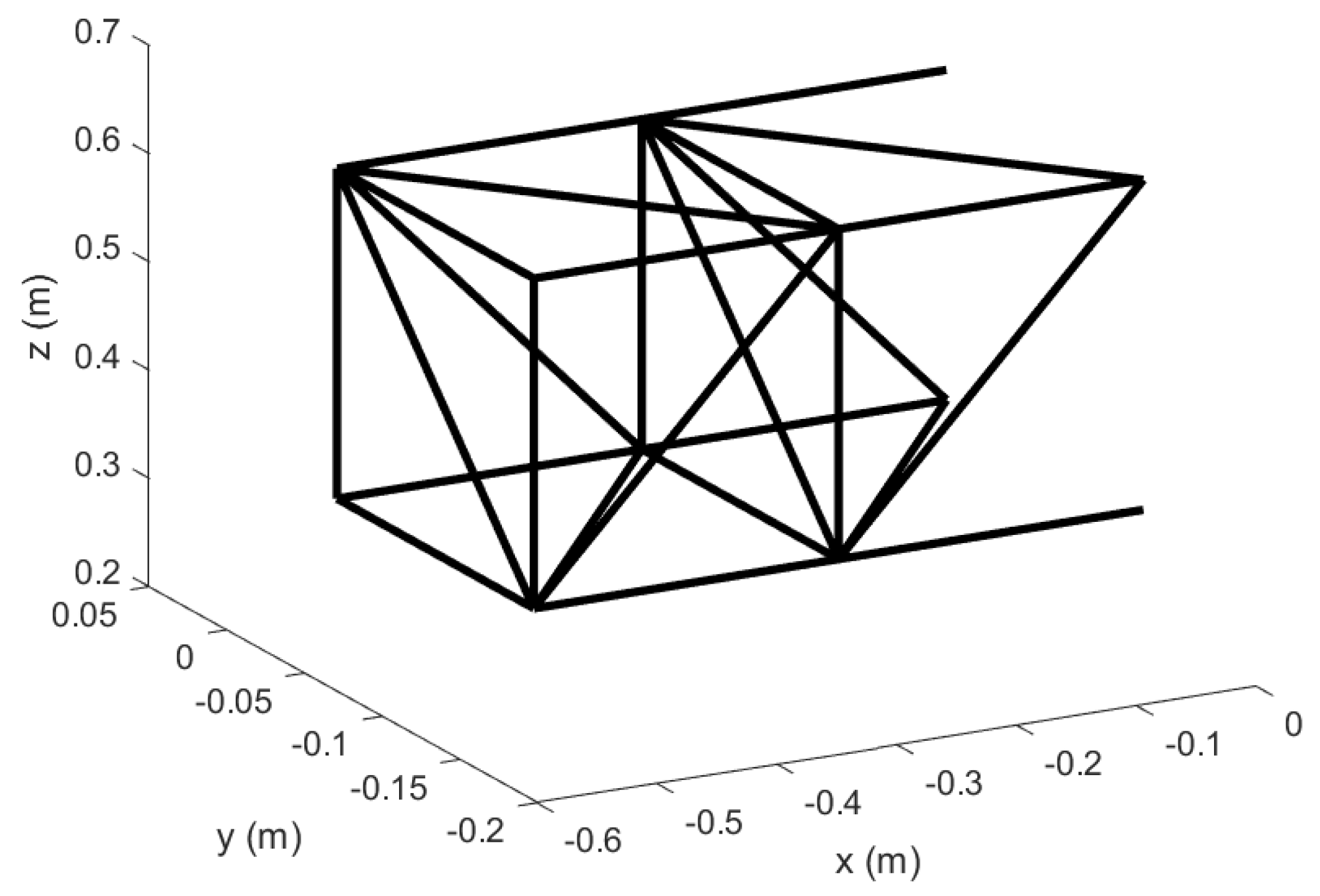
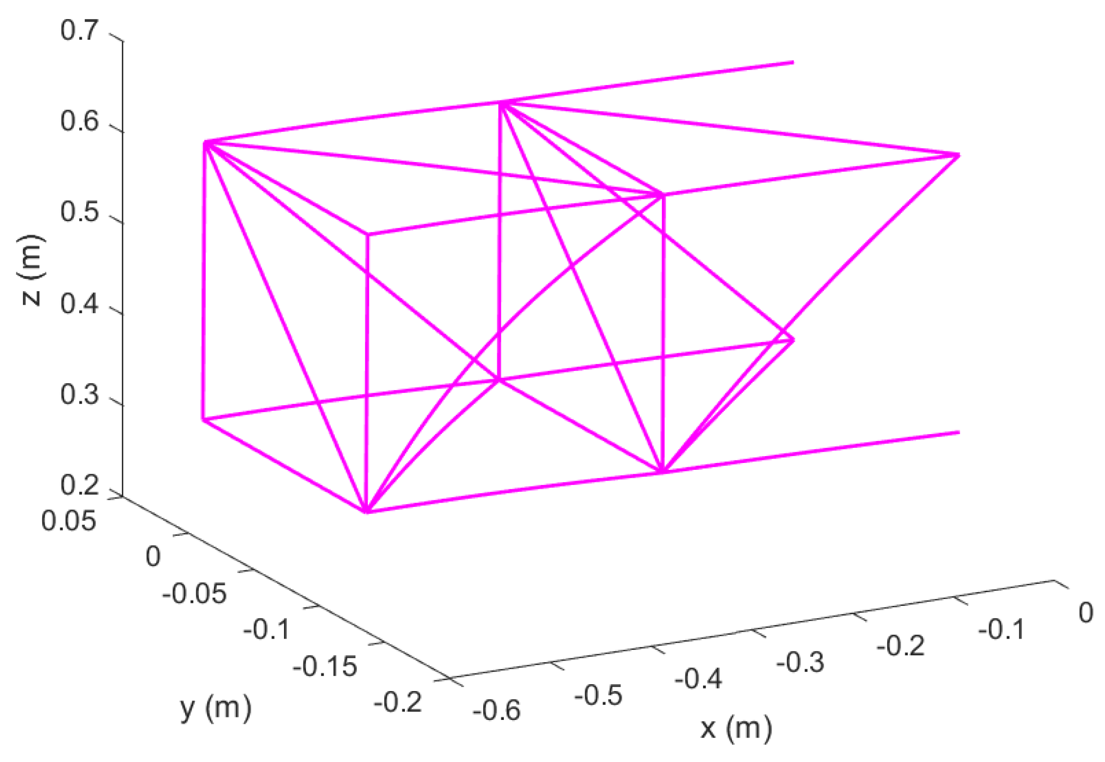
Figure 17.
Un–morphed wing in Topology 1 with hinged ends; original configuration.
Figure 17.
Un–morphed wing in Topology 1 with hinged ends; original configuration.
Figure 18.
Mode 1 of Euler–Bernoulli Beams in Topology 1 with hinged ends; original configuration.
Figure 18.
Mode 1 of Euler–Bernoulli Beams in Topology 1 with hinged ends; original configuration.
Figure 19.
Mode 2 of Euler–Bernoulli Beams in Topology 1 with hinged ends; original configuration.
Figure 19.
Mode 2 of Euler–Bernoulli Beams in Topology 1 with hinged ends; original configuration.
Figure 20.
Mode 3 of Euler–Bernoulli Beams in Topology 1 with hinged ends; original configuration.
Figure 20.
Mode 3 of Euler–Bernoulli Beams in Topology 1 with hinged ends; original configuration.
Figure 21.
Mode 4 of Euler–Bernoulli Beams in Topology 1 with hinged ends; original configuration.
Figure 21.
Mode 4 of Euler–Bernoulli Beams in Topology 1 with hinged ends; original configuration.
Figure 22.
Mode 5 of Euler–Bernoulli Beams in Topology 1 with hinged ends; original configuration.
Figure 22.
Mode 5 of Euler–Bernoulli Beams in Topology 1 with hinged ends; original configuration.
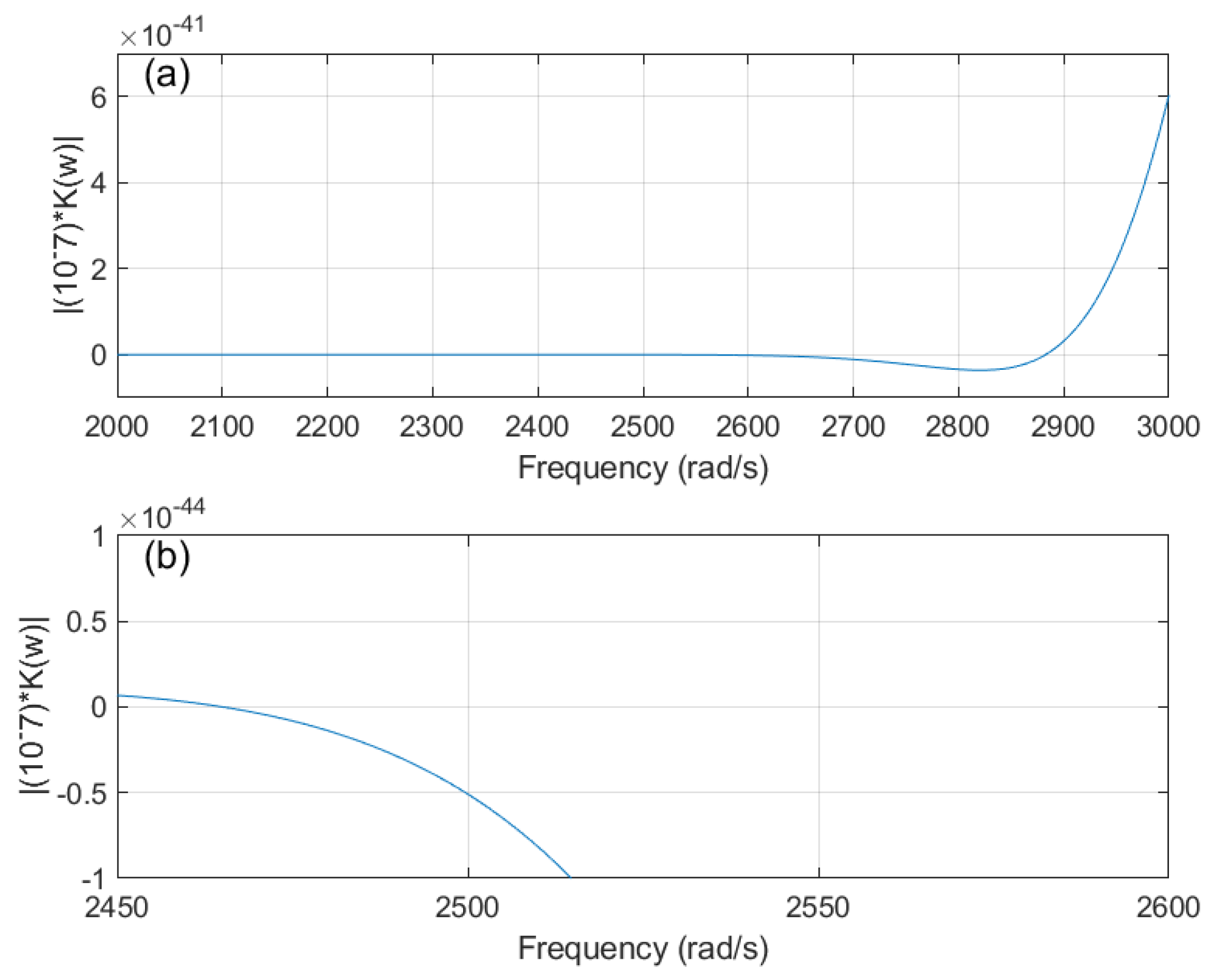
Figure 23.
Dynamic Stiffness Matrix plot of Euler–Bernoulli Beams in Topology 1 with hinged ends using DSM; original configuration (a) a selected region of natural frequencies showing zero–crossing at the 10th natural frequency (b) a detailed section showing zero–crossing at the 9th natural frequency.
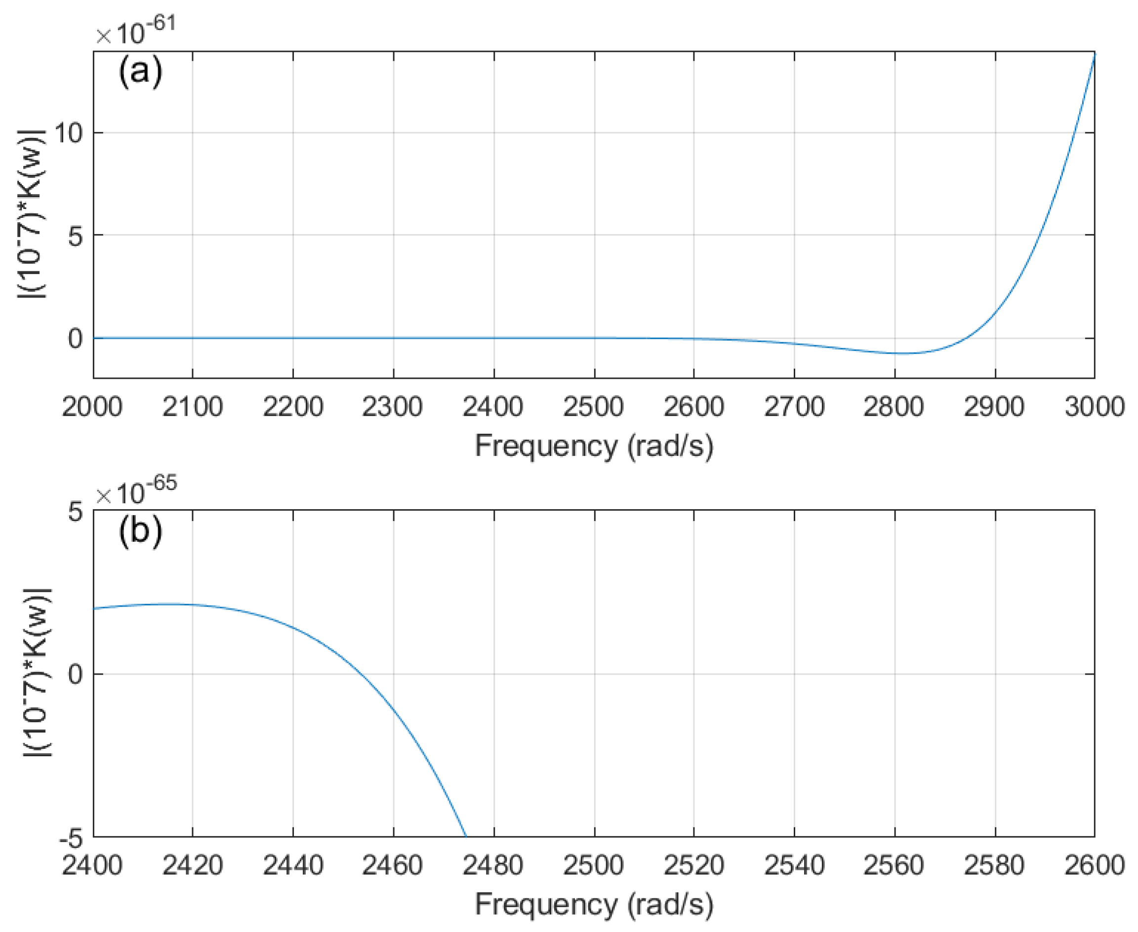
Figure 24.
Mode Plot of Timoshenko beams in Topology 1 with hinged ends using DSM; original configuration (a) a selected region of natural frequencies showing zero–crossing at the 10th natural frequency (b) a detailed section showing zero–crossing at the 9th natural frequency.
Figure 24.
Mode Plot of Timoshenko beams in Topology 1 with hinged ends using DSM; original configuration (a) a selected region of natural frequencies showing zero–crossing at the 10th natural frequency (b) a detailed section showing zero–crossing at the 9th natural frequency.
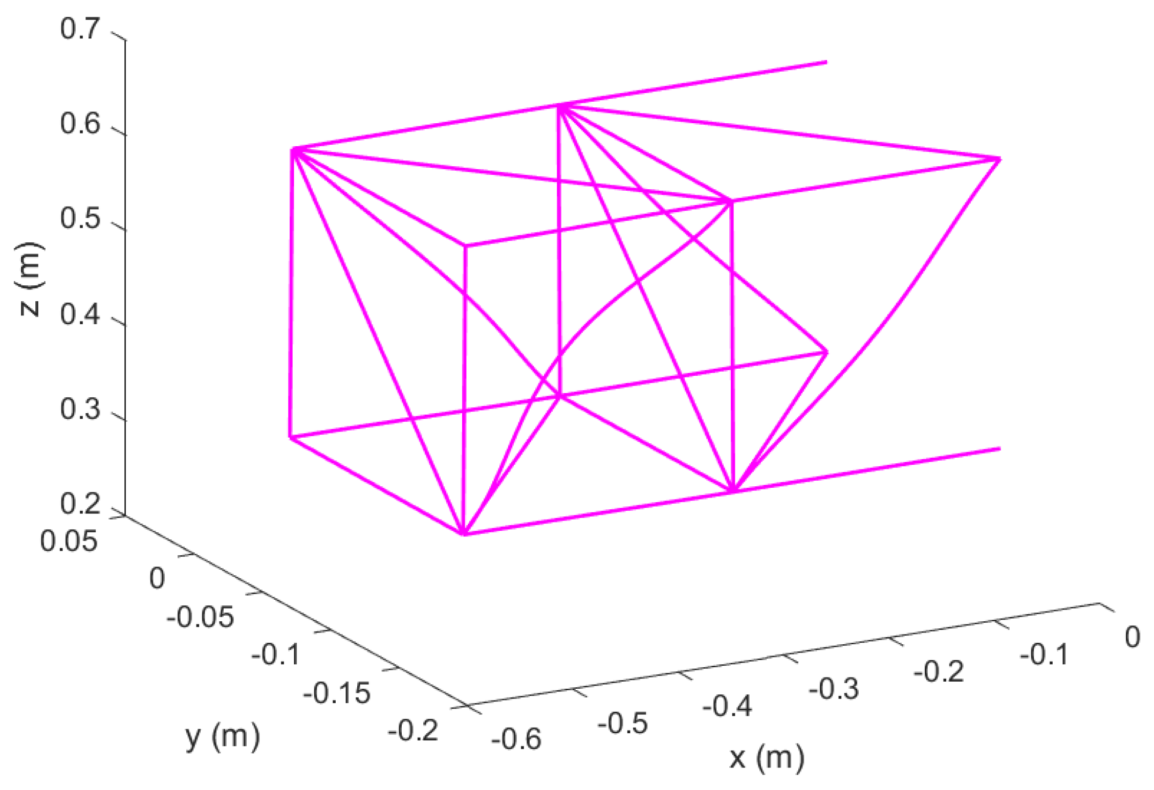
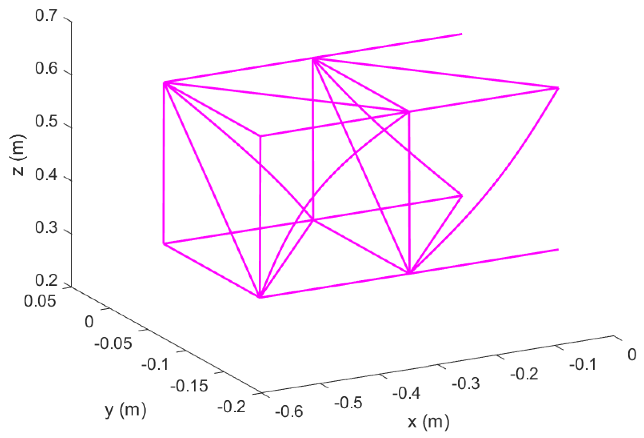
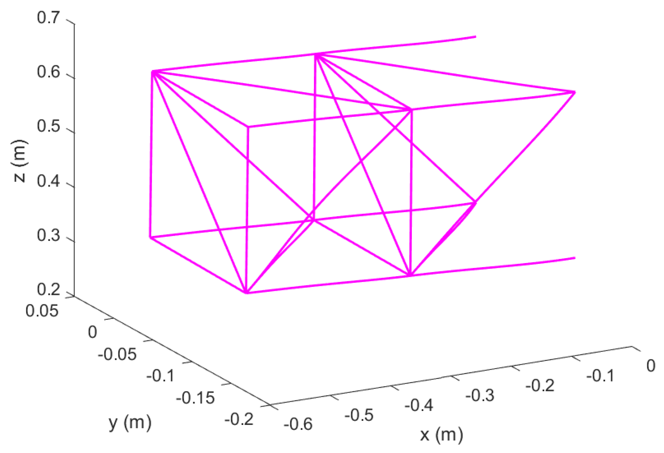
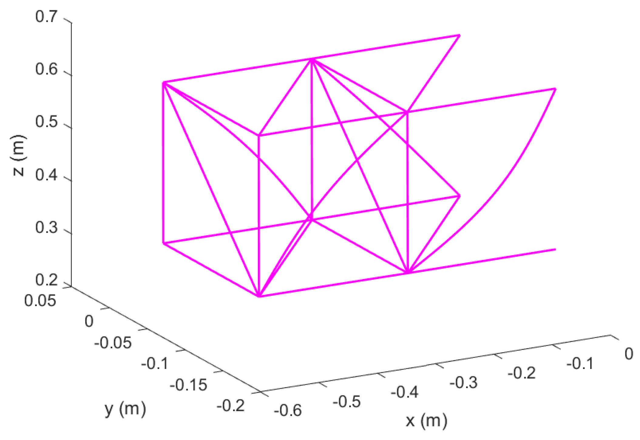
Figure 25.
Un–morphed wing in Topology 1 with hinged ends; original configuration.
Figure 25.
Un–morphed wing in Topology 1 with hinged ends; original configuration.
Figure 26.
Mode 1 of Timoshenko beams in Topology 1 with hinged ends; original configuration.
Figure 26.
Mode 1 of Timoshenko beams in Topology 1 with hinged ends; original configuration.
Figure 27.
Mode 2 of Timoshenko beams in Topology 1 with hinged ends; original configuration.
Figure 27.
Mode 2 of Timoshenko beams in Topology 1 with hinged ends; original configuration.
Figure 28.
Mode 3 of Timoshenko beams in Topology 1 with hinged ends; original configuration.
Figure 28.
Mode 3 of Timoshenko beams in Topology 1 with hinged ends; original configuration.
Figure 29.
Mode 4 of Timoshenko beams in Topology 1 with hinged ends; original configuration.
Figure 29.
Mode 4 of Timoshenko beams in Topology 1 with hinged ends; original configuration.
Figure 30.
Mode 5 of Timoshenko beams in Topology 1 with hinged ends; original configuration.
Figure 30.
Mode 5 of Timoshenko beams in Topology 1 with hinged ends; original configuration.
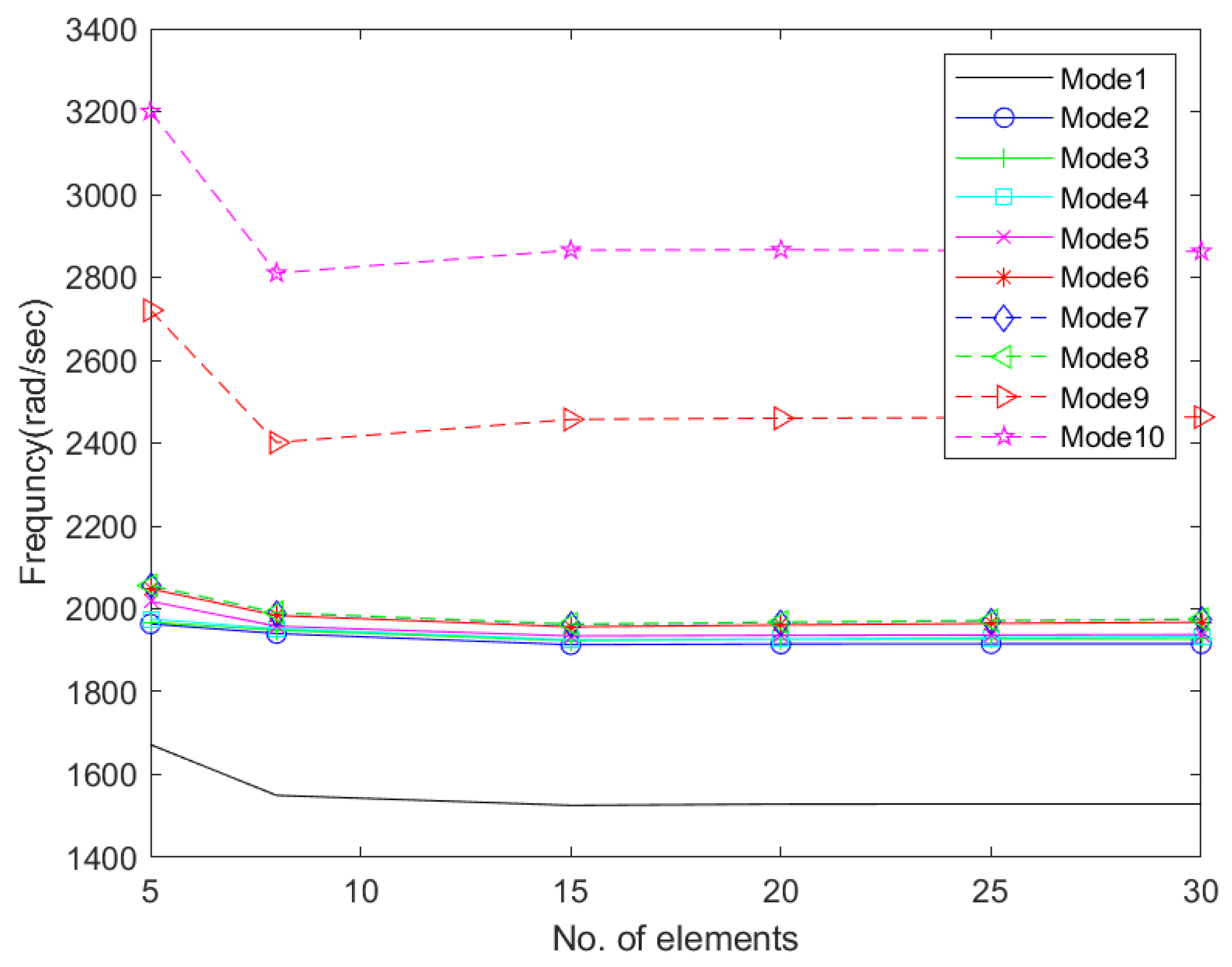
Figure 31.
Convergence of natural frequencies of Timoshenko beams in Topology 1 with hinged ends.
Figure 31.
Convergence of natural frequencies of Timoshenko beams in Topology 1 with hinged ends.
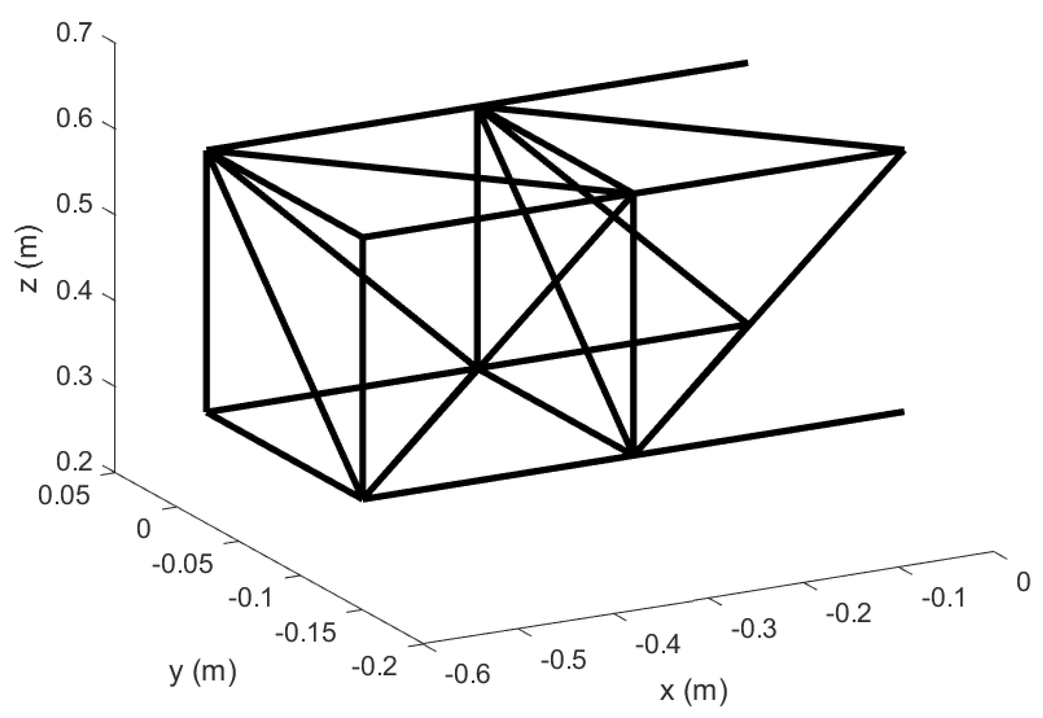
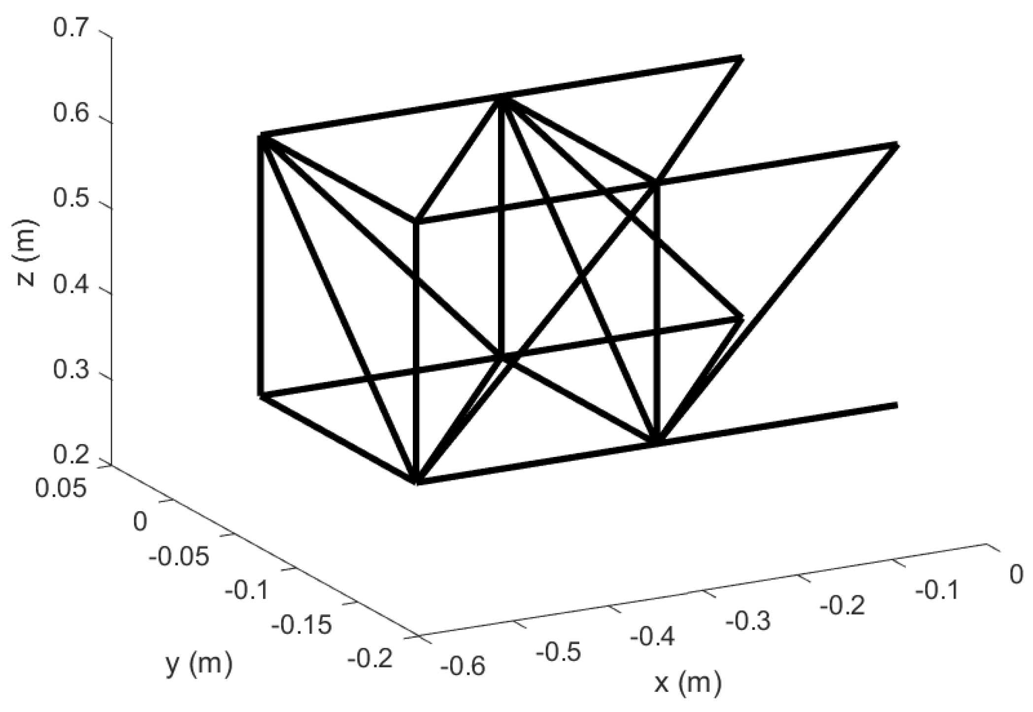
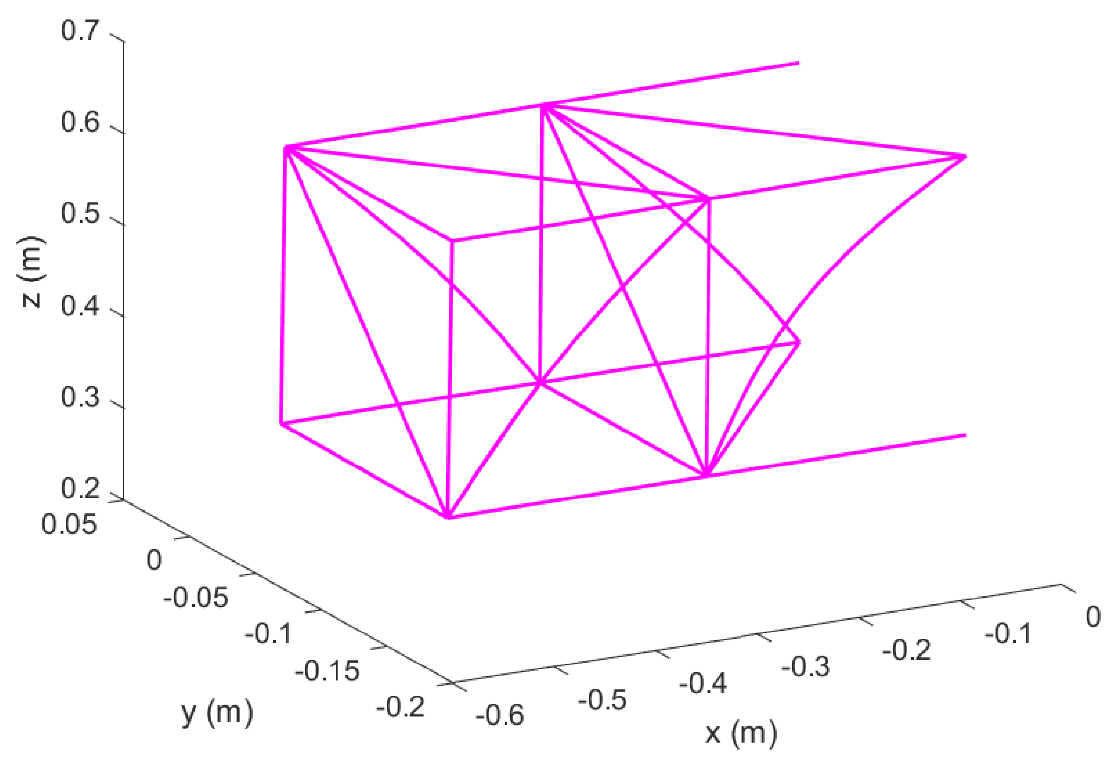
Figure 32.
Spanwise Expanded wing in Topology 1 with hinged ends; morphed configuration.
Figure 32.
Spanwise Expanded wing in Topology 1 with hinged ends; morphed configuration.
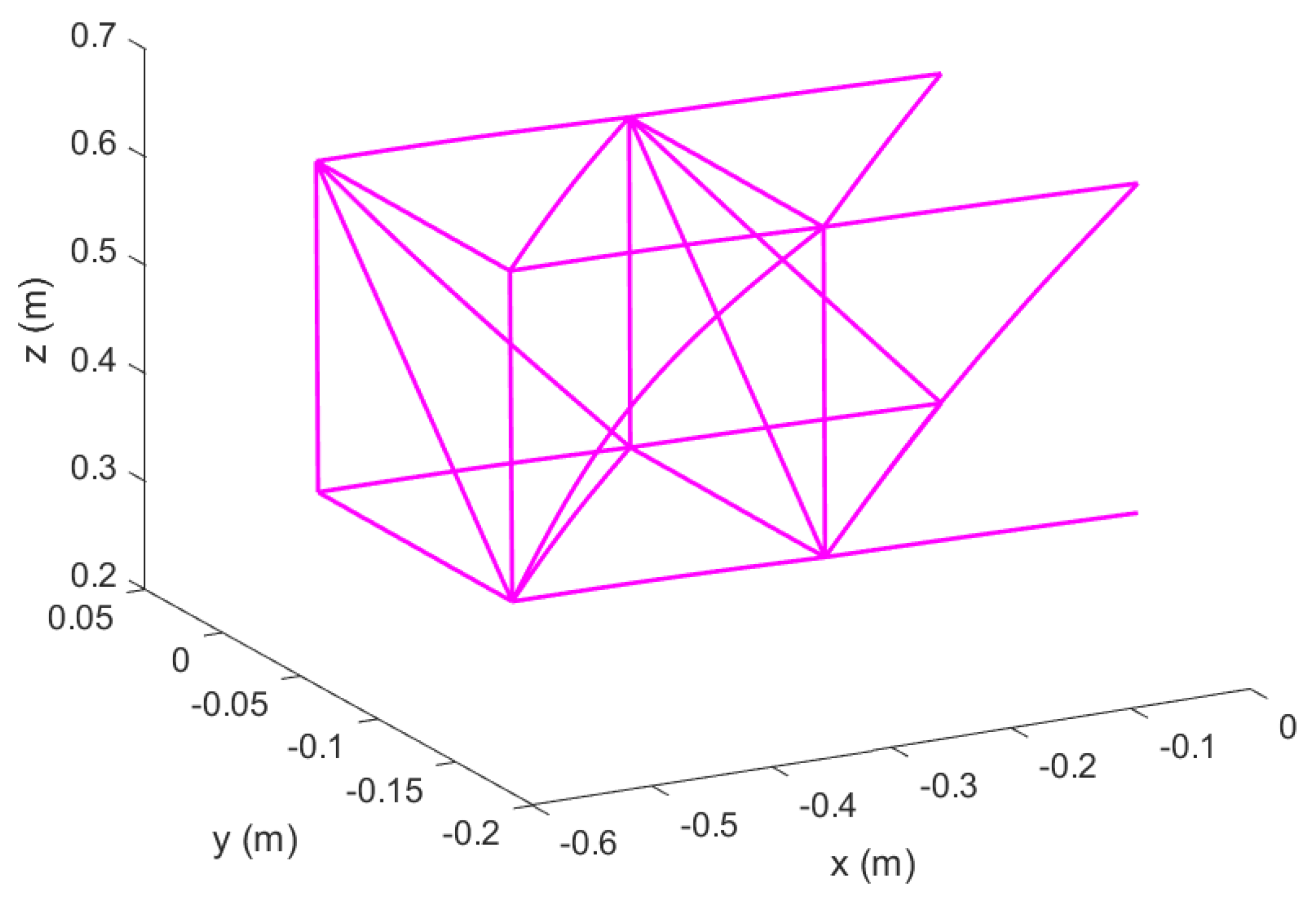
Figure 33.
Mode 1 of Timoshenko beams in Topology 1 with hinged ends; spanwise expanded configuration.
Figure 33.
Mode 1 of Timoshenko beams in Topology 1 with hinged ends; spanwise expanded configuration.
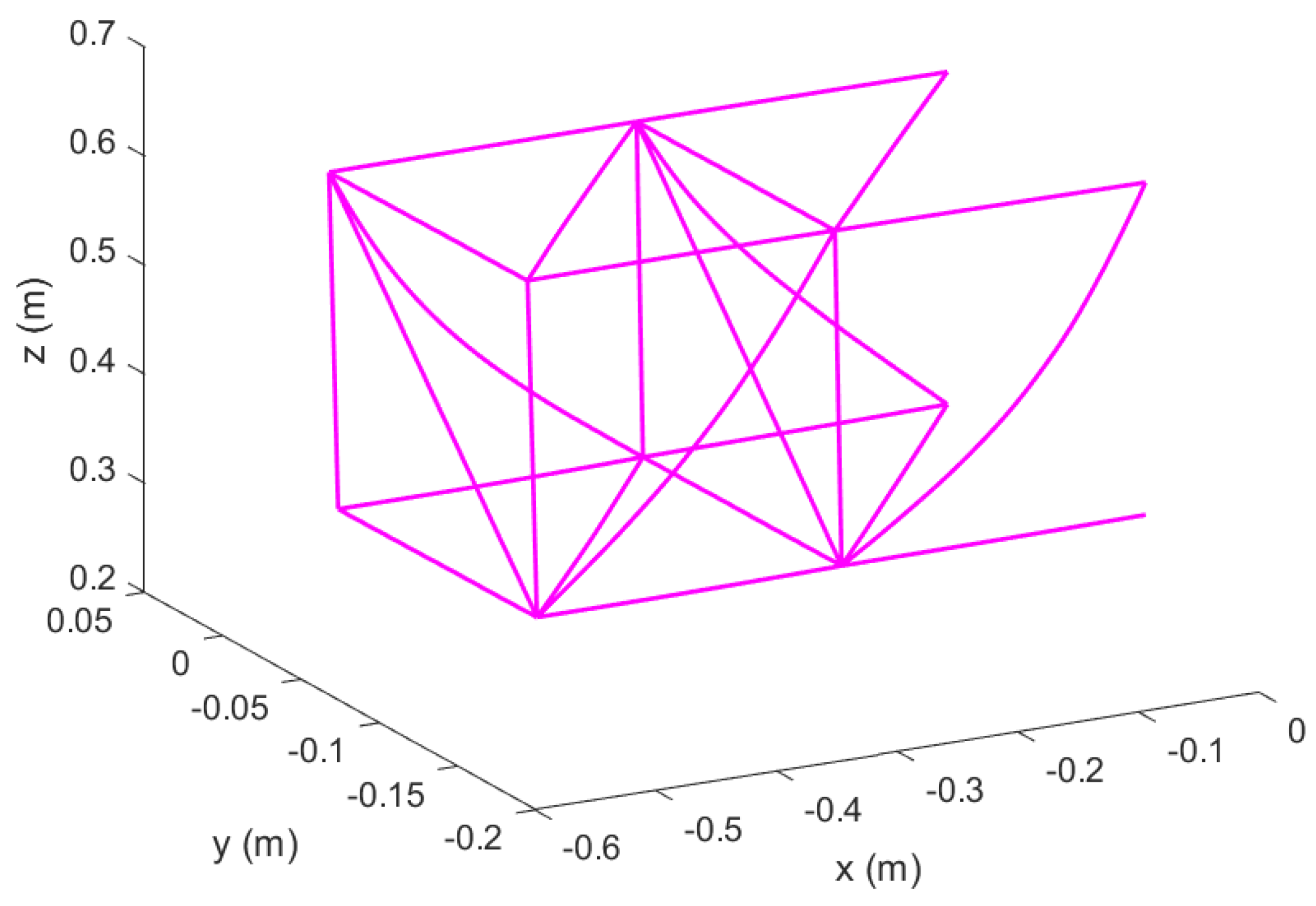
Figure 34.
Mode 2 of Timoshenko beams in Topology 1 with hinged ends; spanwise expanded configuration.
Figure 34.
Mode 2 of Timoshenko beams in Topology 1 with hinged ends; spanwise expanded configuration.
Figure 35.
Mode 3 of Timoshenko beams in Topology 1 with hinged ends; spanwise expanded configuration.
Figure 35.
Mode 3 of Timoshenko beams in Topology 1 with hinged ends; spanwise expanded configuration.
Figure 36.
Mode 4 of Timoshenko beams in Topology 1 with hinged ends; spanwise expanded configuration.
Figure 36.
Mode 4 of Timoshenko beams in Topology 1 with hinged ends; spanwise expanded configuration.
Figure 37.
Mode 5 of Timoshenko beams in Topology 1 with hinged ends; spanwise expanded configuration.
Figure 37.
Mode 5 of Timoshenko beams in Topology 1 with hinged ends; spanwise expanded configuration.
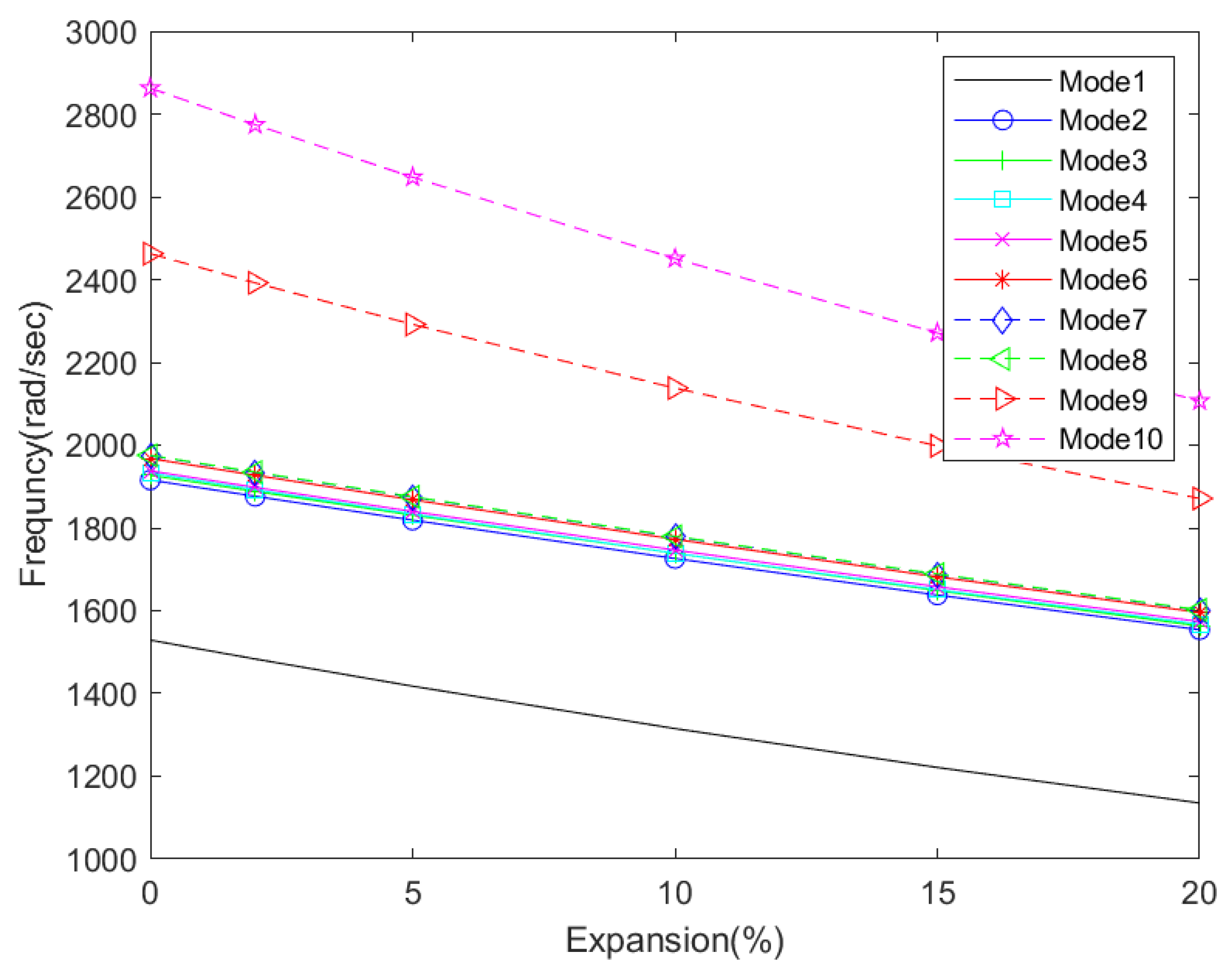
Figure 38.
Changes in natural frequencies of Timoshenko beams with spanwise expansion.
Figure 38.
Changes in natural frequencies of Timoshenko beams with spanwise expansion.
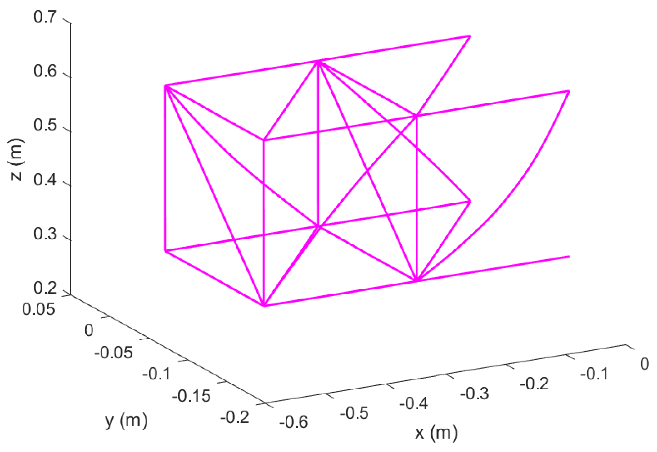
Figure 39.
Un–morphed wing in Topology 2 with hinged ends; original configuration.
Figure 39.
Un–morphed wing in Topology 2 with hinged ends; original configuration.
Figure 40.
Mode 1 of Timoshenko beams in Topology 2 with hinged ends; original configuration.
Figure 40.
Mode 1 of Timoshenko beams in Topology 2 with hinged ends; original configuration.
Figure 41.
Mode 2 of Timoshenko beams in Topology 2 with hinged ends; original configuration.
Figure 41.
Mode 2 of Timoshenko beams in Topology 2 with hinged ends; original configuration.
Figure 42.
Mode 3 of Timoshenko beams in Topology 2 with hinged ends; original configuration.
Figure 42.
Mode 3 of Timoshenko beams in Topology 2 with hinged ends; original configuration.
Figure 43.
Mode 4 of Timoshenko beams in Topology 2 with hinged ends; original configuration.
Figure 43.
Mode 4 of Timoshenko beams in Topology 2 with hinged ends; original configuration.
Figure 44.
Mode 5 of Timoshenko beams in Topology 2 with hinged ends; original configuration.
Figure 44.
Mode 5 of Timoshenko beams in Topology 2 with hinged ends; original configuration.
Table 1.
Wing Morphing and its effect.
Table 1.
Wing Morphing and its effect.
| Morphing Type | Performance Effects | Benefit | Cost |
|---|
| Sweep | Drag-divergence, Mach number | Maneuvers, high-speed flight | Lower lift coefficient, higher weight |
| Cant | Lateral stability | Positive increases roll | Decrease maneuverability |
| Twist | Lift, Drag | Aerodynamic force control | Wing torsional rigidity |
| Span | Aspect Ratio, Wing loading | Shorter span maneuverability | Wing root moment |
Table 2.
Mechanical Properties of Steel.
Table 2.
Mechanical Properties of Steel.
| Material | Density | Modulus of Elasticity | Poisson Ratio | Shear Modulus |
|---|
| | kg/m3 | Pa | | Pa |
|---|
| Low Carbon Steel | 7750.4 | 1.8616 × 10¹¹ | 0.3 | 7.16 × 10¹⁰ |
Table 3.
Natural Frequencies, , of Two Euler–Bernoulli Beams Analysis with Hinged node.
Table 3.
Natural Frequencies, , of Two Euler–Bernoulli Beams Analysis with Hinged node.
| Mode | 1 | 2 | 3 | 4 | 5 | 6 | 7 | 8 | 9 | 10 |
|---|
| FEM | 1781.8 | 1781.8 | 7441 | 7452.5 | 11159 | 11182 | 19234 | 19234 | 24118 | 24257 |
| Ansys | 1684.94 | 1684.94 | 7223.50 | 7223.50 | 10,213.30 | 10,213.30 | 18,794.43 | 18,794.43 | 22,369.11 | 22,369.11 |
| Difference (%) | 5.75 | 5.75 | 3.01 | 3.17 | 9.26 | 9.48 | 2.34 | 2.34 | 7.82 | 8.44 |
Table 4.
Natural Frequencies, of Euler–Bernoulli Beam Analysis with no spherical joint in Topology 1, Original Configuration.
Table 4.
Natural Frequencies, of Euler–Bernoulli Beam Analysis with no spherical joint in Topology 1, Original Configuration.
| Mode | 1 | 2 | 3 | 4 | 5 | 6 | 7 | 8 | 9 | 10 |
|---|
| FEM | 1909.5 | 3471.1 | 3590.5 | 4307.4 | 4372.5 | 4395.3 | 4419 | 4429.5 | 4507.7 | 4850.5 |
| DSM | 1910.4 | 3474.1 | 3586.4 | 4309.1 | 4372.6 | 4387.2 | 4411.6 | 4421.4 | 4509.3 | 4841.3 |
| Difference (%) | 0.05 | 0.09 | 0.119 | 0.04 | 0.0023 | 0.18 | 0.17 | 0.18 | 0.035 | 0.19 |
Table 5.
Natural Frequencies, of Euler–Bernoulli Beam Analysis with Hinged ends in Topology 1, Original Configuration.
Table 5.
Natural Frequencies, of Euler–Bernoulli Beam Analysis with Hinged ends in Topology 1, Original Configuration.
| Mode | 1 | 2 | 3 | 4 | 5 | 6 | 7 | 8 | 9 | 10 |
|---|
| FEM | 1549.6 | 1917.6 | 1923.6 | 1937.1 | 1945.7 | 1950.5 | 1953.3 | 1954.1 | 2498.5 | 2922.1 |
| DSM | 1533.7 | 1914.6 | 1923.3 | 1938 | 1946.8 | 1949.7 | 1949.7 | 1952.6 | 2465.3 | 2881.3 |
Difference
(%) | 1.04 | 0.16 | 0.02 | 0.05 | 0.06 | 0.04 | 0.18 | 0.08 | 1.35 | 1.42 |
Table 6.
Natural Frequencies, of Timoshenko beam Analysis with Hinged ends in Topology 1, original configuration.
Table 6.
Natural Frequencies, of Timoshenko beam Analysis with Hinged ends in Topology 1, original configuration.
| Mode | 1 | 2 | 3 | 4 | 5 | 6 | 7 | 8 | 9 | 10 |
|---|
| FEM | 1528.9 | 1915.7 | 1927.2 | 1932.4 | 1937.7 | 1967.6 | 1974.5 | 1975.4 | 2462.6 | 2862.4 |
| DSM | 1530.8 | 1905.8 | 1911.6 | 1926.3 | 1935.1 | 1938 | 1940.9 | 1940.9 | 2453.6 | 2872.6 |
Difference
(%) | 0.12 | 0.52 | 0.82 | 0.32 | 0.13 | 1.53 | 1.73 | 1.78 | 0.37 | 0.36 |
Table 7.
Natural Frequencies, of Timoshenko beam Analysis with Hinged ends in Topology 1, spanwise expanded configuration.
Table 7.
Natural Frequencies, of Timoshenko beam Analysis with Hinged ends in Topology 1, spanwise expanded configuration.
| Mode | 1 | 2 | 3 | 4 | 5 | 6 | 7 | 8 | 9 | 10 |
|---|
| FEM | 1276.6 | 1690.3 | 1702.2 | 1703 | 1710.5 | 1735.7 | 1741.8 | 1742.6 | 2080.4 | 2376.8 |
Table 8.
Change of Natural Frequencies, of Timoshenko beam Analysis with Hinged ends in Topology 1, with spanwise expansion.
Table 8.
Change of Natural Frequencies, of Timoshenko beam Analysis with Hinged ends in Topology 1, with spanwise expansion.
| Mode Number | Expansion (%) |
|---|
| 0 | 2 | 5 | 10 | 15 | 20 |
|---|
| Mode 1 | 1528.9 | 1483.4 | 1417.7 | 1315.2 | 1221.3 | 1135.4 |
| Mode 2 | 1915.7 | 1876.4 | 1818.8 | 1726.2 | 1637.9 | 1553.9 |
| Mode 3 | 1927.2 | 1888.1 | 1830.8 | 1738.7 | 1648.6 | 1562.9 |
| Mode 4 | 1932.4 | 1892.4 | 1833.6 | 1738.9 | 1650.8 | 1567.3 |
| Mode 5 | 1937.7 | 1897.9 | 1839.7 | 1746.5 | 1657.9 | 1573.6 |
| Mode 6 | 1967.6 | 1927.2 | 1867.8 | 1772.5 | 1681.8 | 1595.7 |
| Mode 7 | 1974.5 | 1933.9 | 1874.4 | 1778.7 | 1687.7 | 1601.2 |
| Mode 8 | 1975.4 | 1934.8 | 1875.2 | 1779.6 | 1688.5 | 1602 |
| Mode 9 | 2462.6 | 2392 | 2291.7 | 2137.8 | 1998.4 | 1871.2 |
| Mode 10 | 2862.4 | 2774 | 2647.2 | 2450.6 | 2271 | 2106.7 |
Table 9.
Natural Frequencies, of Timoshenko beam Analysis with Hinged ends in Topology 2, original configuration.
Table 9.
Natural Frequencies, of Timoshenko beam Analysis with Hinged ends in Topology 2, original configuration.
| Mode | 1 | 2 | 3 | 4 | 5 | 6 | 7 | 8 | 9 | 10 |
|---|
| FEM | 1547.3 | 1892.4 | 1923 | 1928.4 | 1937.8 | 1964.7 | 1974.5 | 1975.2 | 2480.1 | 2703.4 |


