Article

Differential Quadrature Method for Fully Intrinsic Equations of Geometrically Exact Beams

College of Aerospace Engineering, Nanjing University of Aeronautics and Astronautics, Nanjing 210016, China
*
Author to whom correspondence should be addressed.
Aerospace 2022, 9(10), 596; https://doi.org/10.3390/aerospace9100596
Submission received: 5 August 2022 / Revised: 18 September 2022 / Accepted: 3 October 2022 / Published: 12 October 2022
(This article belongs to the Special Issue Structural Dynamics and Control)

Abstract

:
In this paper, a differential quadrature method of high-order precision (DQ−Pade), which is equivalent to the generalized Pade approximation for approximating the end of a time or spatial interval, is used to solve nonlinear fully intrinsic equations of beams. The equations are a set of first-order differential equations with respect to time and space, and the explicit unknowns of the equations involve only forces, moments, velocity and angular velocity, without displacements and rotations. Based on the DQ−Pade method, the spatial and temporal discrete forms of fully intrinsic equations were derived. To verify the effectiveness and applicability of the proposed method for discretizing the fully intrinsic equations, different examples available in the literatures were considered. It was found that when using the DQ−Pade method, the solutions of the intrinsic beam equations are obviously superior to those found by some other usual algorithms in efficiency and computational accuracy.

1. Introduction

Due to the high aspect ratio of a rotor blade, which is usually regarded as a beam-like structure, beam theory has been a very important part of helicopter rotor dynamics modeling and analysis. The blade will have medium or large deflection in complex working environments, which leads to the nonlinear characteristics of the aeroelastic response analysis of the helicopter rotor. Among the many beam theories describing these nonlinear behaviors, the large deformation beam theory has attracted the most attention. It has only a small strain assumption and no restriction on displacements or rotations.
At present, the large deformation beam theory has been applied in many fields, and lots of beam models have been developed. They can be classified according to their solution methods. It was found that there are three categories: displacement-based methods [1], mixed-form methods [2,3] and stress-based methods [4,5]. The main advantage of displacement-based methods is the ease of applying geometric boundary conditions with them. However, they are computationally expensive due to the higher-order nonlinear terms. Even with high-order truncation, the complete formula has to be written over several pages. Mixed-form methods establish the kinematics equation by mixing the rotation and displacement variables with the generalized velocity and strain measures. Lagrange multipliers are used to apply the constitutive and kinematic relations to the governing equations in the mixed formula. Differently from the displacement-based theory and the mixed formula theory, there is no displacement, nor any rotation variables, in the stress-based formula. Green and Laws [6] coined the term “fully intrinsic” for this concept. The fully intrinsic theory was originally proposed by Hegemier and Nair [7]. In 2003, Hodges [4] reconsidered it on the basis of [2] and developed the fully intrinsic equations of geometrically exact beams, which only include forces, moments, velocity and angular velocity. The displacements and rotations can be obtained by recovering them in the post-processing. Due to no truncation in the derivation process, these compact equations are complete and accurate, and the maximum nonlinearity (the highest order of the nonlinear terms in the equations) is only two. Palacios and Cesnik [8] compared the numerical efficiency and ease of use of these three different methods for the analysis of aircraft structure, aeroelastic characteristics, and flight dynamics.
Patil and Hodges [9] analyzed the nonlinear aeroelastic characteristic of wings with a high aspect ratio using the fully intrinsic method. Patil and Althoff [10] presented an energy-continuous Galerkin method for solving the fully intrinsic equations, which can obtain a high precision solution with a low computational cost. However, the Galerkin method was also found to face some difficulties in practical applications, such as time-consuming integration and an inability to deal with spatial discontinuity. Patil and Hodges [11] proposed the concept of the variable-order finite-element Galerkin method. They found that the third-order finite element offers a particularly good balance of accuracy, computational efficiency, and applicability to general problems. Sotoudeh and Hodges [12] developed an incremental method for solving the fully intrinsic equations of statically indeterminate structures. They [13] also extended the application of fully intrinsic theory to more general configurations by establishing different types of fully intrinsic boundary conditions. Khaneh, Masjedi, and Ovesy [14,15] investigated the static analysis method by discretizing the fully intrinsic equations using the Chebyshev collocation method. Tashaorian et al. [16] established non-local, fully intrinsic equations for non-beam-like structures whose one-dimensional structure length is close to the two-dimensional cross-section size, which breaks through the limitation that the fully intrinsic equations can only be used for modeling slender structures. Byeonguk et al. [17] used the exponential function to replace the Rodrigues parameters to represent the finite rotation, and realized the absolute non-singularity expression in the equations, and therefore, the numerical realization of solving the equations became more compact.
The fully intrinsic equations developed by Hodges are the differential equations of first-order partial derivatives in time and space. Usually, two steps are needed to discretize them: the first is to discretize the equations of motion in the spatial domain to obtain the first-order partial differential equations about time; the second is to discretize the equations of motion in the time domain to obtain the algebraic equations, which can be solved directly. There are four commonly used methods for spatial discretization in the literature which the reader can consult. The first is the finite difference method. Hodges [2] used the central difference scheme to discretize the equations in the spatial domain, and mentioned that this method has second-order accuracy. The second is the Galerkin method, which was presented by Patil [10] using Legendre polynomials as weighting functions to establish integral equations. The third method is the Chebyshev collocation method. Khaneh, Masjedi, and Ovesy [14,15] used this method to discretize static intrinsic equations. The last method is the differential quadrature (DQ) method that has been used more recently.
It was proposed by Bellman and Casti [18] in 1971. The basic principle is that the derivative of a function at a specific point can be approximated as a weighted linear summation of the function values at all discrete points in the entire domain. Bert [19] first applied the method to the mechanical analysis of structural elements, and found that the method has the advantages of a simple formula, convenient use, less computation, and high precision. However, with the deepening of research and applications, researchers found that when the number of discrete points is large, the numerical ill-condition will appear when calculating the weighting coefficients. This disadvantage limited the application of the DQ method. Shu and Richards [20,21] overcame the shortcoming by introducing the generalized differential quadrature (GDQ) method based on Lagrange polynomial vector space. By using the GDQ method, the weighting coefficients of arbitrary-order derivatives are calculated using simple algebraic formulas. A notable feature of the GDQ method is that there are no limits to the type and number of discrete points. Oleg et al. [22] constructed a multi-layer wavelet collocation method which uses the Gaussian wavelet function as the interpolation basis function, and the collocation points are selected by dichotomy. An adaptive multi-layer wavelet configuration method [23] and a fast, adaptive wavelet configuration method [24] were presented by the same group. Chen [25] proposed the concept of the differential quadrature element method, which discretizes the domain into several regular sub-domains to deal with irregular boundaries. Wei et al. [26] found that the differential quadrature element method is more effective at dealing with higher-order derivative problems. Fung [27,28] pointed out that the accuracy and stability of the DQ method in the time domain depend on the locations of the sampling discrete points. By using appropriately distributed discrete points, the accuracy of the end value of the time interval can be improved to 2N-1 or 2N (N is the maximum order of polynomials), which is better than the commonly used uniformly spaced point and Chebyshev–Gauss–Lobatto point distribution. They proved that this terminal approximation is equivalent to the generalized Pade approximation.
Amoozgar and Shahverdi [29] firstly applied the differential quadrature method to solve the fully intrinsic equations of a geometrically exact beam. They found that the GDQ method can obtain more accurate results with a lesser computational cost than the traditional finite element method. Based on GDQ method, they also analyzed the dynamic stability of the beam under following forces [30] and the aeroelastic stability of the hingeless rotor [31]. Tashaorian et al. [16] used the GDQ method for the spatial discretization of non-local fully intrinsic equations.
For the first-order partial differential equations with respect to time obtained after the space discretization of the fully intrinsic equations, the difference algorithms [2,10,32] are commonly used to solve them recursively. These algorithms often need to go through a time-consuming recursion process when solving the aeroelastic response of the rotor, especially when solving the steady-state periodic response of the rotor. Borri [33] also pointed out the shortcomings of these algorithms in solving the steady-state response of the rotor’s aeroelasticity: since these algorithms are solved step by step, recursively, an initial value is required. For the nonlinear equations of aeroelasticity, it may be difficult to find an initial value related to a specific periodic solution. Therefore, he proposed that in the time-discrete process of the equations of motion, a set of algebraic equations should be derived by substituting periodic boundary value conditions, so that the nonlinear steady-state periodic solution of the rotor aeroelasticity can be obtained directly.
In this paper, the space-time discretization of the fully intrinsic beam equations is carried out on the basis of a differential quadrature method of high-order precision, and the new calculation formulas for solving the responses of the fully intrinsic dynamic equations of the beam are presented. The validity and applicability of the formulas proposed in this paper are verified by static analysis and modal calculation of the cantilever beam, and the calculation of the beam’s dynamic response, including the transient response and periodic steady-state response.

2. Fully Intrinsic Beam Equations

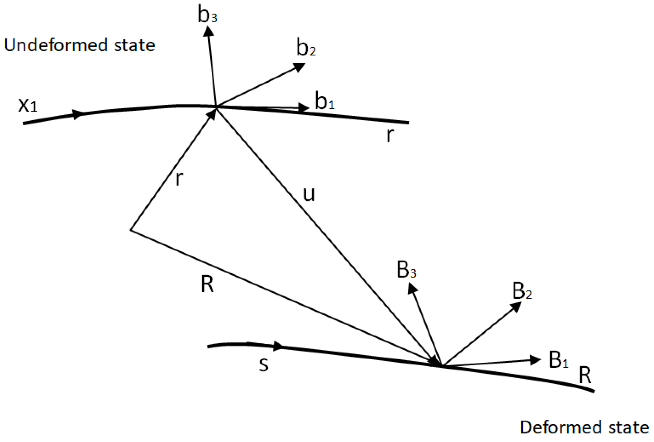
Figure 1 shows the undeformed and deformed states of the beam. At each point on the axis of the undeformed beam, a reference coordinate system b ( x 1 ) is introduced. At each point along the axis of the deformed beam, a reference coordinate system B ( x 1 ) is introduced. All variables involved in the fully intrinsic equations are expressed in the coordinate system b and B . The equations can be expressed in a compact form as
F B + ( k ˜ + κ ˜ ) F B + f B = P ˙ B + Ω ˜ B P B M B + ( k ˜ + κ ˜ ) M B + ( e ˜ 1 + γ ˜ ) F B + m B = H ˙ B + Ω ˜ B H B + V ˜ B P B V B + ( k ˜ + κ ˜ ) V B + ( e ˜ 1 + γ ˜ ) Ω B = γ ˙ B Ω B + ( k ˜ + κ ˜ ) Ω B = κ ˙ B
Here, (   ) represents the partial derivative with respect to the reference axis of the undeformed beam coordinate system, and ( · ) represents the partial derivative with respect to time. F ( x , t ) and M ( x , t ) represent the force and moment of the beam section, respectively. P ( x , t ) and H ( x , t ) represent the linear momentum and angular momentum of the beam section, respectively. γ ( x , t ) and κ ( x , t ) represent the generalized force and moment strains of the beam, respectively. V ( x , t ) and Ω ( x , t ) represent the linear and angular velocities of the beam section, respectively. f ( x , t ) and m ( x , t ) represent the external force and moment acting on the beam, respectively. k is the initial twist/curvature of the beam that expressed in the undeformed coordinate system b . (   ) ˜ is the cross-product operator, and for k = k 1 k 2 k 3 T , the operator can be expressed as
k ˜ = 0 k 3 k 2 k 3 0 k 1 k 2 k 1 0
The first two equations in Equations (1) are partial differential equations of linear and angular momentum equilibrium. The latter two are partial differential equations for the kinematic equations, which were derived from the generalized strain-displacement and generalized velocity-displacement equations. This process essentially eliminates the displacement and rotation variables, leaving the equation with only intrinsic quantities.
γ κ = R S S T T F M P H = μ Δ μ ξ ˜ μ ξ ˜ I F M
Equations (3) are the equations for the beam constitutive relation and the generalized velocity-momentum relation. R ( x ) , T ( x ) , and S ( x ) are the flexibility characteristic constants of the beam profile. This linear constitutive relation is valid for small-strain cases. μ ( x ) , ξ ( x ) , and I ( x ) represent the beam’s linear density, centroid offset (the centroid of the profile relative to the reference axis), and the moment of inertia per unit length, respectively. Equations (1) and (3) constitute a complete set of differential equations for first-order partial derivatives in time and space.

3. Space-Time Discretization of Fully Intrinsic Equations

3.1. Discretization in the Spatial Domain

To solve the above equations, space discretization must be carried out first. The essence of spatial discretization is to eliminate the derivative terms. The DQ method, which has received much attention in recent years, approximates the derivative term as the weighted linear summation of the function values at all discrete points along the domain. Therefore, the computation of the weight coefficients is very important, which depends on the distribution of discrete points. The approximate solution at the end of time interval obtained by the discrete point distribution used in the [27,28] is equivalent to the approximate solution obtained by using the Pade approximation. Its characteristic is that the accuracy of the approximate solution at the inner points of the domain is no different from it is other points on the distribution, both of which are p -order ( p is the maximum order of the polynomials). However, the accuracy at the terminal node can be improved to 2 p where the additional parameter μ = 1 (the format is non-dissipative at the high-frequency regime).
This paper firstly adopts this discrete points’ distribution to discretize the spatial domain equations, and this differential discretization method is called the DQ−Pade method in this paper. The n th derivative of the function f ( x ) with respect to the spatial direction x can be expressed as
( n ) f x ( n ) = f x ( n ) ( x i ) = k = 1 N W i k ( n ) f ( x k ) , n = 1 , , N
Here, W i k ( n ) is the weight coefficient, and the algebraic expression is as follows:
W i k ( 1 ) = M ( 1 ) ( x i ) ( x i x k ) M ( 1 ) ( x k ) , i , k = 0 , 1 , . , N b u t i k W i i ( 1 ) = M ( 2 ) ( x i ) 2 M ( 1 ) ( x k ) , i = 0 , 1 , . , N
Among them, M , M ( 1 ) , and M ( 2 ) can be calculated by the respective following formulas:
M ( ζ ) = ζ N + 1 W 1 ζ W 2 ζ 2 W 3 ζ 3 W N ζ N M ( 1 ) ( ζ ) = ( N + 1 ) ζ N W 1 2 W 2 ζ 3 W 3 ζ 2 N W N ζ N 1 M ( 2 ) ( ζ ) = N ( N + 1 ) ζ N 1 2 W 2 6 W 3 ζ N ( N 1 ) W N ζ N 2
where
W k = ( 1 ) N k N ! N ! ( N + k 2 ) ! ( k 1 ) ! ( k 1 ) ! ( N + 1 k ) ! ( 2 N ) !   ·   2 ( N + μ ( k 1 ) ) 1 + μ ,   0 μ 1
The calculation method of discrete points is obtained by the following formula:
ζ N W 1 W 2 ζ W 3 ζ 2 W N ζ N 1 = 0
By taking the root of the above equation, N discrete points can be obtained. Figure 2 shows the distribution at N = 9 . As can be seen in the figure, the discrete points are not evenly distributed, and nodal points (0 or 1) are not included. Therefore, when introducing boundary conditions V 0 , Ω 0 , F L , and M L , Equation (5) should be used to directly calculate the weight coefficient W i 0 of the start point value or to calculate W i L of end point after some transformations. Thus, the spatial derivative terms in Equation (1) are written as
V i = k = 1 N W i k V k + W i 0 V 0 Ω i = k = 1 N W i k Ω k + W i 0 Ω 0 F i = k = 1 N W i k F k + W i L F L   M i = k = 1 N W i k M k + W i L M L  
By substituting Equation (9) into Equation (1), the spatial discretization of the intrinsic equations based on DQ−Pade method can be expressed as
k = 1 N W i k F k + ( k ˜ i + κ ˜ i ) F i + f i + W i L F L = P ˙ i + Ω ˜ i P i k = 1 N W i k M k + ( k ˜ i + κ ˜ i ) M i + ( e ˜ 1 + γ ˜ i ) F i + m i + W i L M L = H ˙ i + Ω ˜ i H i + V ˜ i P i k = 1 N W i k V k + ( k ˜ i + κ ˜ i ) V i + ( e ˜ 1 + γ ˜ i ) Ω i + W i 0 V 0 = γ ˙ i k = 1 N W i k Ω k + ( k ˜ i + κ ˜ i ) Ω i + W i 0 Ω 0 = κ ˙ i
In Equations (9) and (10), the subscripts containing i or k are variables corresponding to discrete points x i or x k . Arrange the equations with respect to the time term, and then a set of differential equations with respect to time, which are the same in form as other spatial discretization methods, is obtained:
A j i q ˙ i + B j i q i + C j i k q i q k + D j = 0
where q is the vector of unknown intrinsic variables, A and B are linear coefficient matrices. C is a nonlinear coefficient matrix. D is the external load vector, which also contains intrinsic dynamic boundary conditions V 0 , Ω 0 , F L , and M L .
It is worth mentioning that the DQ−Pade method can also be used to discretize the equations of displacements and rotations recovering from the intrinsic variables (Hodges [5]):
u = C T ( e 1 + γ ) e 1 k ˜ u θ = ( Δ + 1 2 θ ˜ + 1 4 θ θ T ) ( κ + k C k )
where
C = [ 1 ( 1 / 4 ) θ T θ ] Δ θ ˜ + ( 1 / 2 ) θ θ T 1 + ( 1 / 4 ) θ T θ
The equations after using DQ−Pade discretization can be expressed as
k = 1 N W i k u k + W i 0 u 0 C i T ( e 1 + γ i ) + e 1 + k ˜ i u i = 0 k = 1 N W i k θ k + W i 0 θ 0 ( Δ + 1 2 θ ˜ i + 1 4 θ i θ i T ) ( κ i + k i C i k i ) = 0
Here, θ is the Rodriguez parameter representing the rotation matrix. u 0 and θ 0 are the geometric boundary conditions. The discretized equations are algebraic equations containing nonlinearity and need to be solved iteratively.

3.2. Discretization in the Time Domain

DQ−Pade was originally derived for the solution of time-domain responses and has been successfully applied in time-domain problems [20,21]. Therefore, it is naturally used in this paper to discretize the first-order partial differential equation with respect to time obtained after space discretization. Compared with the traditional recursive method, this paper presents the global format of the DQ−Pade method, which can get the responses of all discrete time points at once.
If there are M + 1 time points ( t 0 , t 1 , , t M ) in a time domain T , t i ( i = 1 , , M ) is the best approximation of the time discrete point calculated by Equations (7) and (8). Additionally, t 0 is the start point of the time domain T . Thus, the time derivative term q ˙ in the discrete Equation (11) can be discretized by the DQ−Pade method:
q ˙ ( t ) = k = 1 M W i k q k + W i 0 q 0 i n i t i a l
where the weight coefficients W can be calculated using Equation (5)–(8); q 0 i n i t i a l is the initial condition. Substitute Equation (15) into (11). Then, the following equation is obtained:
A k = 1 M W i k q k + A W i 0 q 0 i n i t i a l + B q i + C ( q i ) q i + D i = 0 , i = 1 , , M
Equation (16) can also be written in matrix form as
A W 11 + B + C ( q 1 ) A W 12 A W 13 A W 1 M A W 21 A W 22 + B + C ( q 2 ) A W 23 A W 2 M A W 31 A W 32 A W 33 + B + C ( q 3 ) A W 3 M A W M 1 A W M 2 A W M 3 A W M M + B + C ( q M ) q 1 q 2 q 3 q M + A W 10 q 0 i n i t i a l A W 20 q 0 i n i t i a l A W 30 q 0 i n i t i a l A W M 0 q 0 i n i t i a l + D 1 D 2 D 3 D M = 0
The above equation can be written in a simplified form:
A t o t a l q t o t a l + A 0 q 0 i n i t i a l + D t o t a l = 0
This is the initial value formula for the time-discrete solution based on the DQ−Pade method. Given the initial condition q 0 i n i t i a l , the responses at all discrete time points can be solved at one time.
If the time domain T is a period, the steady-state periodic response of the intrinsic equations is required. For this case, it is difficult to give the initial value q 0 i n i t i a l satisfying the final steady-state periodic response when Equation (18) is still used. Therefore, it is necessary to deduce the discrete formula with consideration of the periodic boundary condition
q 0 = q T
Here, q T can be obtained by polynomial interpolation:
q T = L 0 ( 1 ) q 0 + L 1 ( 1 ) q 1 + + L M ( 1 ) q M
where L k is the Lagrange interpolation polynomial. Substitute Equation (19) into (18) to get
q 0 b o u n d a r y = l 1 q 1 + + l M q M   ,   l i = L i / ( 1 L 0 )
q 0 b o u n d a r y is the constraint condition of periodic boundary value problems. Bring it into Equation (16) and write it in matrix form:
A W 11 + B + C ( q 1 ) A W 12 A W 13 A W 1 M A W 21 A W 22 + B + C ( q 2 ) A W 23 A W 2 M A W 31 A W 32 A W 33 + B + C ( q 3 ) A W 3 M A W M 1 A W M 2 A W M 3 A W M M + B + C ( q M ) q 1 q 2 q 3 q M + A W 10 l 1 A W 10 l 2 A W 10 l 3 A W 10 l M A W 20 l 1 A W 20 l 2 A W 20 l 3 A W 20 l M A W 30 l 1 A W 30 l 2 A W 30 l 3 A W 30 l M A W M 0 l 1 A W M 0 l 2 A W M 0 l 3 A W M 0 l M q 1 q 2 q 3 q M + D 1 D 2 D 3 D M = 0
Similarly, the equation can be simplified as
A t o t a l q t o t a l + A 0 q 0 b o u n d a r y + D t o t a l = 0
Equation (23) is the periodic boundary value formula based on the DQ−Pade method for a time discrete solution. Like the initial value formula of Equation (17) and (18), the derived algebraic equations contain nonlinear terms, C . Therefore, it is necessary to solve the algebraic equations via nonlinear iteration, e.g., a Newton iteration method. To get the function’s values at other points along the domain, Lagrange polynomial interpolation can be used.

3.3. DQ−Pade Element Method

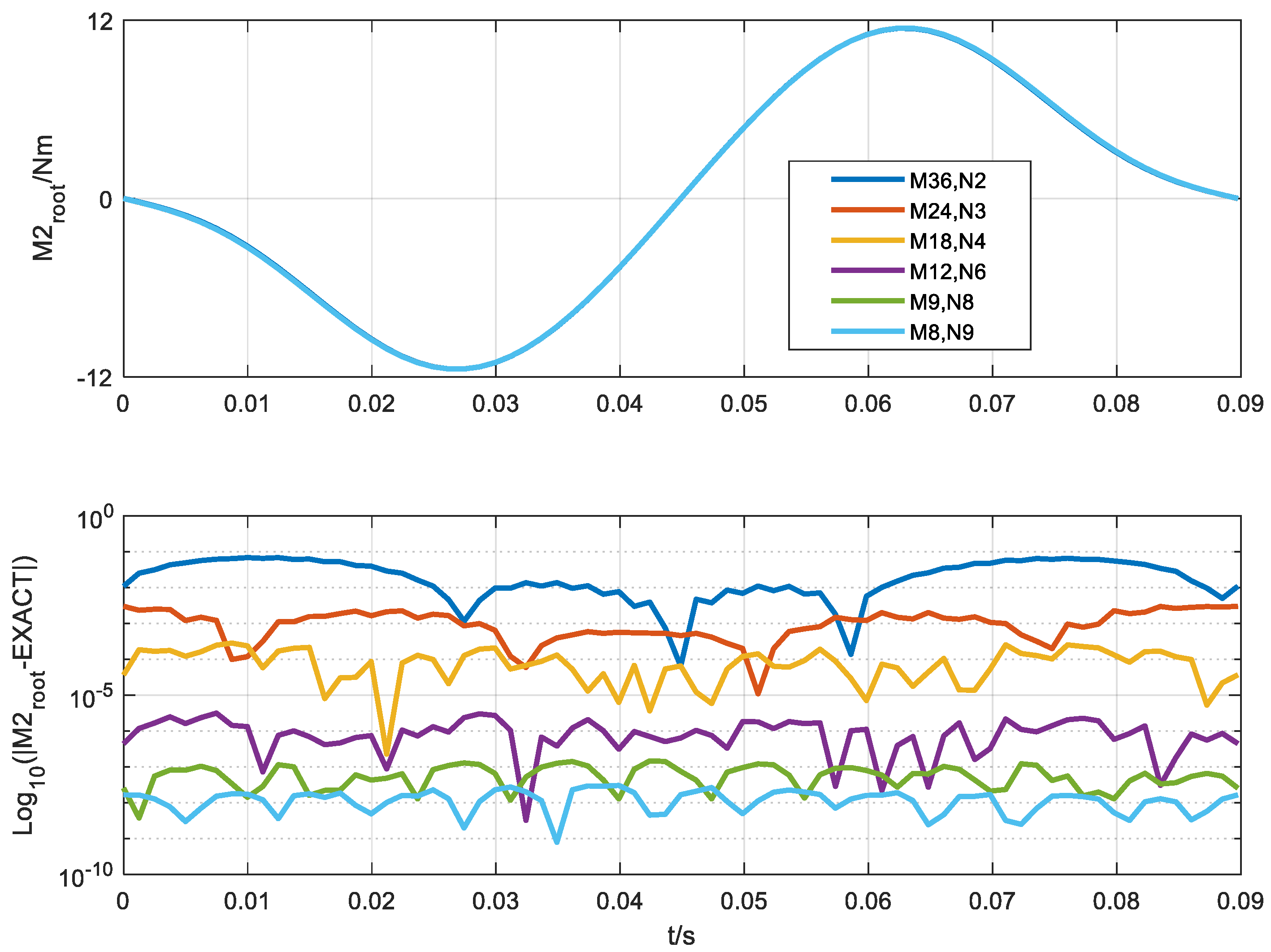
It can be seen in the space discrete equation, Equation (10), and the time discrete equation, Equations (18) and (23), that the coefficient matrixes of the equations are fully matrixes (each element of a matrix has a nonzero value). When dealing with large-scale problems, such as rapid changes or discontinuities in spatial or time domains, the quantity of discrete points needs to be increased, and then the cost of storing and operating the coefficient matrix will increase rapidly, reducing the computational efficiency. Another reason that can be seen in Equation (8) is that when the discrete number N is large, it is difficult to find the root of the formula, which leads to a decrease in the calculation accuracy of the weight coefficient. Meanwhile, there are more nodal points in the domain, which is beneficial to the accuracy of the DQ−Pade method to some extent. Therefore, it is necessary to divide the entire time/space domain into multiple sub-domains, similarly to the finite element method. Additionally, the sub-domains are connected through the weight coefficients of the public points.
If M elements are divided in the spatial domain, the spatial discrete Equation (10) is transformed into
k = 1 N W i k F k m + ( k ˜ i m + κ ˜ i m ) F i m + f i m + W i L ( k = 1 N L k ( 0 ) F k m + 1 ) = P ˙ i m + Ω ˜ i m P i m k = 1 N W i k M k m + ( k ˜ i m + κ ˜ i m ) M i m + ( e ˜ 1 + γ ˜ i m ) F i m + m i m + W i L ( k = 1 N L k ( 0 ) M k m + 1 ) = H ˙ i m + Ω ˜ i m H i m + V ˜ i m P i m   k = 1 N W i k V k m + ( k ˜ i m + κ ˜ i m ) V i m + ( e ˜ 1 + γ ˜ i m ) Ω i m + W i 0 ( k = 0 N L k ( 1 ) V k m 1 ) = γ ˙ i m k = 1 N W i k Ω k m + ( k ˜ i m + κ ˜ i m ) Ω i m + W i 0 ( k = 1 N L k ( 1 ) Ω k m 1 ) = κ ˙ i m
The boundary conditions can be expressed as
k = 0 N L k ( 1 ) V k m 1 = V 0 ,   k = 1 N L k ( 1 ) Ω k m 1 = Ω 0 ,   when   m = 1 k = 1 N L k ( 0 ) F k m + 1 = F L ,   k = 1 N L k ( 0 ) M k m + 1 = M L ,   when   m = M
When M elements are divided in the time domain, the initial value Equation (17) is transformed into
AW 11 + B + C ( q 1 1 ) AW 1 N AW N 1 AW N N + B + C ( q N 1 ) AW 10 L 1 ( 1 ) AW 10 L N ( 1 ) AW 11 + B + C ( q 1 2 ) AW 1 N AW N 0 L 1 ( 1 ) AW N 0 L N ( 1 ) AW N 1 AW N N + B + C ( q N 2 ) AW 10 L 1 ( 1 ) AW 10 L N ( 1 ) AW 11 + B + C ( q 1 M ) AW 1 N AW N 0 L 1 ( 1 ) AW N 0 L N ( 1 ) AW N 1 AW N N + B + C ( q N M ) q 1 1 q N 1 q 1 2 q N 2 q 1 M q N M + D 1 1 + AW 10 q 0 i n i t i a l D N 1 + AW N 0 q 0 i n i t i a l D 1 2 D N 2 D 1 M D N M = 0
and the boundary value formula, Equation (22), is transformed into
AW 11 + B + C ( q 1 1 ) AW 1 N AW 10 L 1 ( 1 ) AW 10 L N ( 1 ) AW N 1 AW N N + B + C ( q N 1 ) AW N 0 L 1 ( 1 ) AW N 0 L N ( 1 ) AW 10 L 1 ( 1 ) AW 10 L N ( 1 ) AW 11 + B + C ( q 1 2 ) AW 1 N AW N 0 L 1 ( 1 ) AW N 0 L N ( 1 ) AW N 1 AW N N + B + C ( q N 2 ) AW 10 L 1 ( 1 ) AW 10 L N ( 1 ) AW 11 + B + C ( q 1 M ) AW 1 N AW N 0 L 1 ( 1 ) AW N 0 L N ( 1 ) AW N 1 AW N N + B + C ( q N M ) q 1 1 q N 1 q 1 2 q N 2 q 1 M q N M + D 1 1 D N 1 D 1 2 D N 2 D 1 M D N M = 0
The main diagonal matrix block in Equation (26) and (27) is the coefficient matrix of each element, and the sub-diagonal matrix is the connection coefficient matrix formed by each element through the public point (the connecting point of two elements). The matrix block in the upper right corner of the Equation (27) is a connected coefficient matrix formed by the periodic boundary condition. The initial value condition is reflected in the first sub-vector in the total load vector of Equation (26).
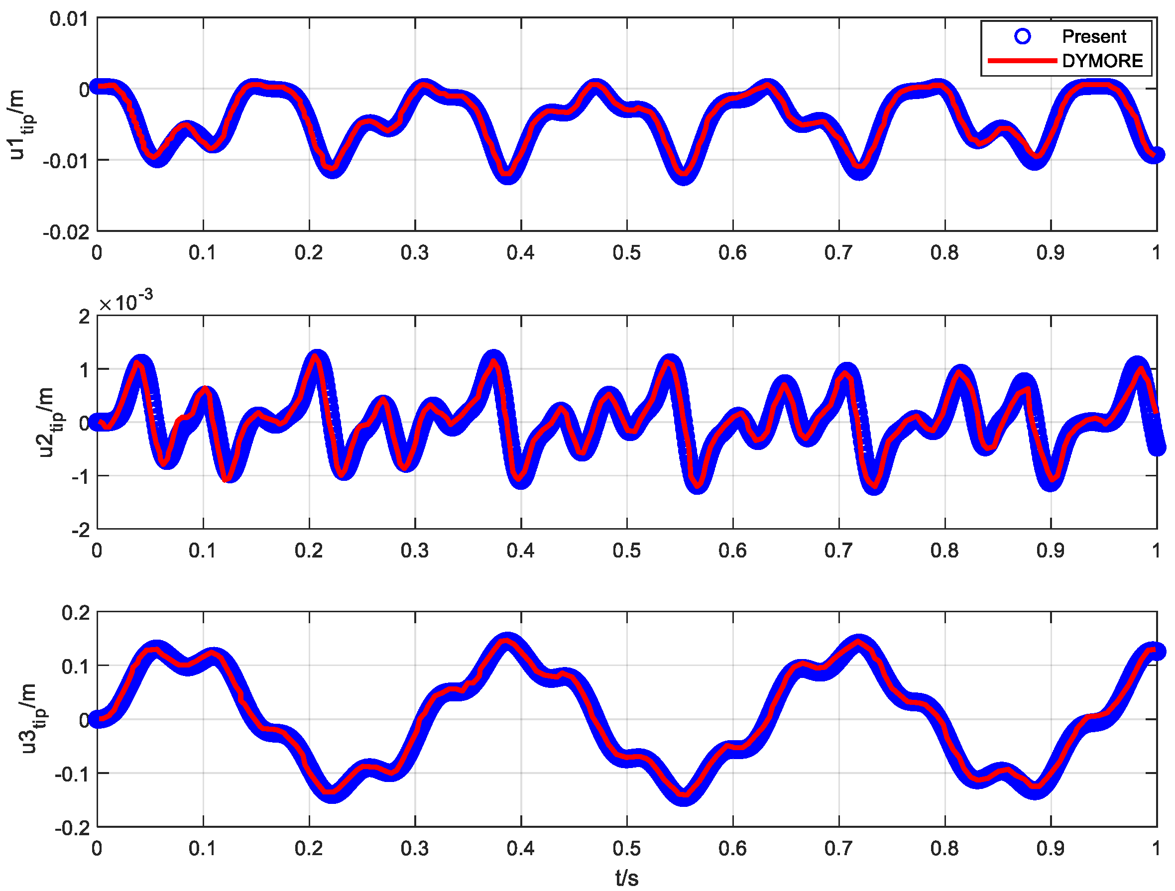
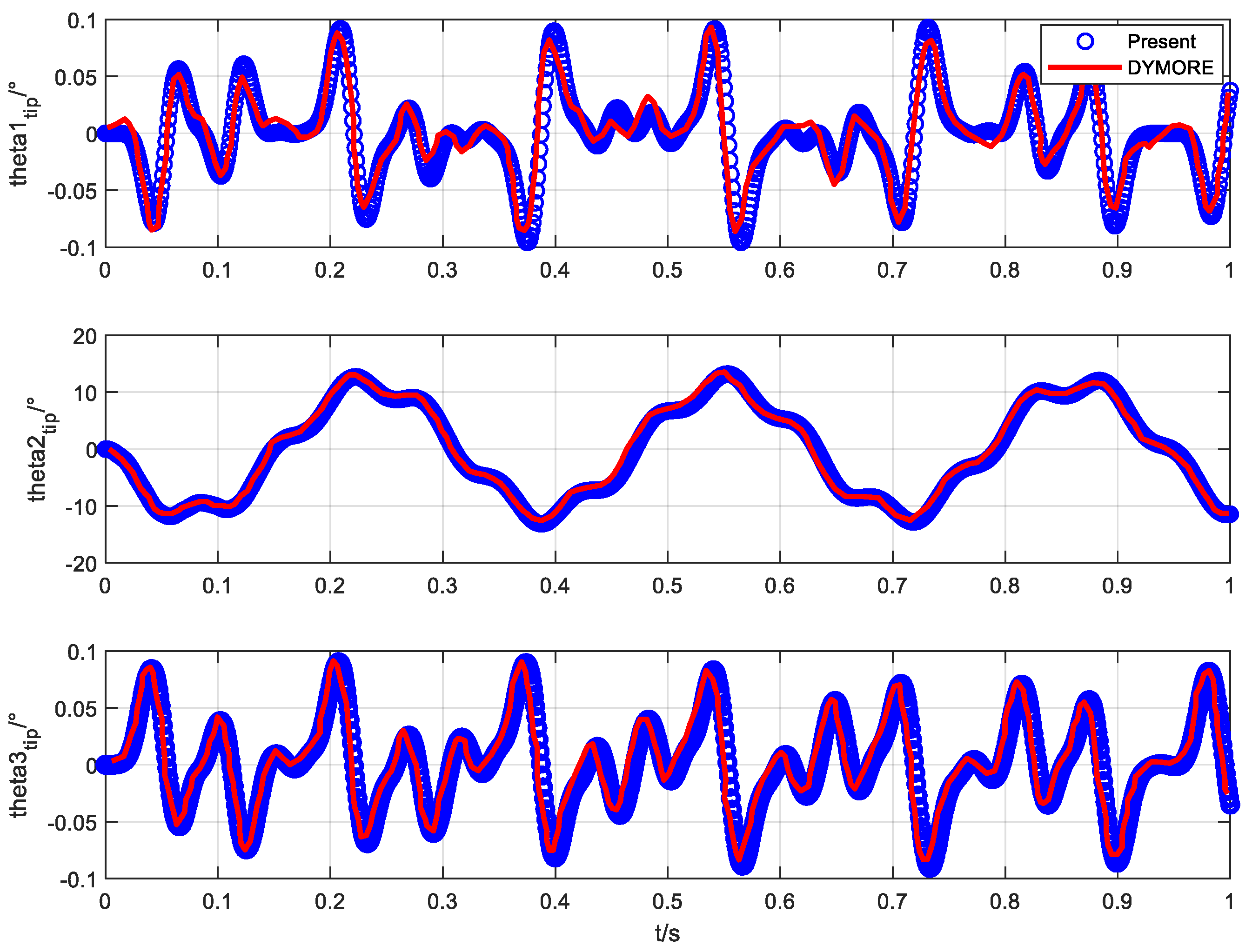
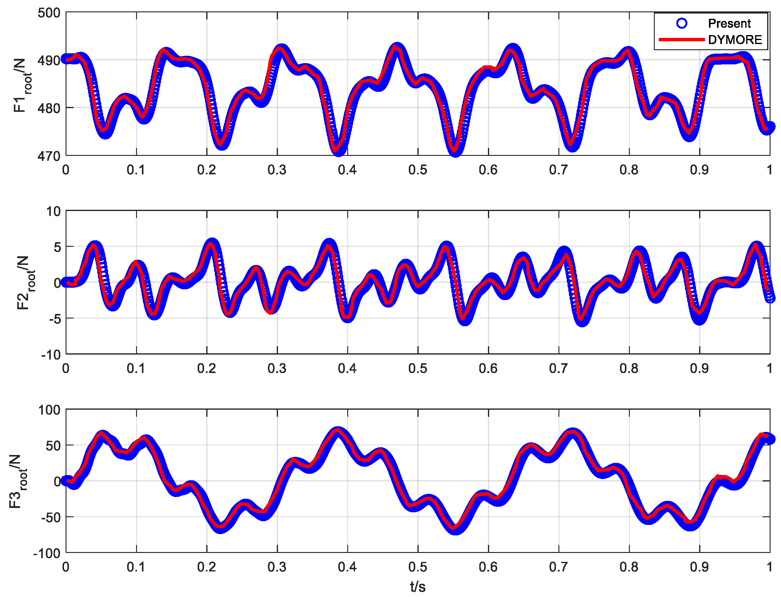
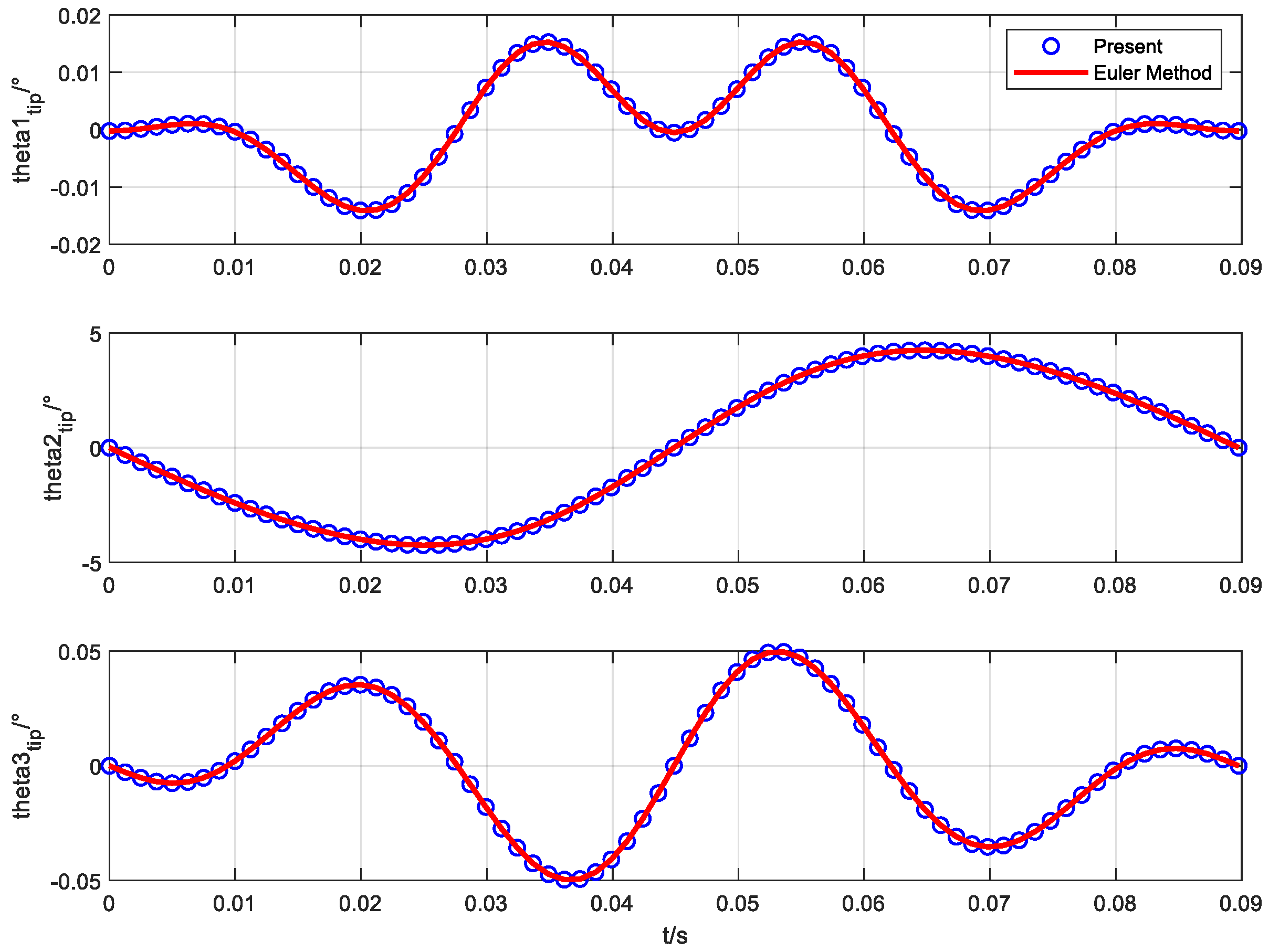
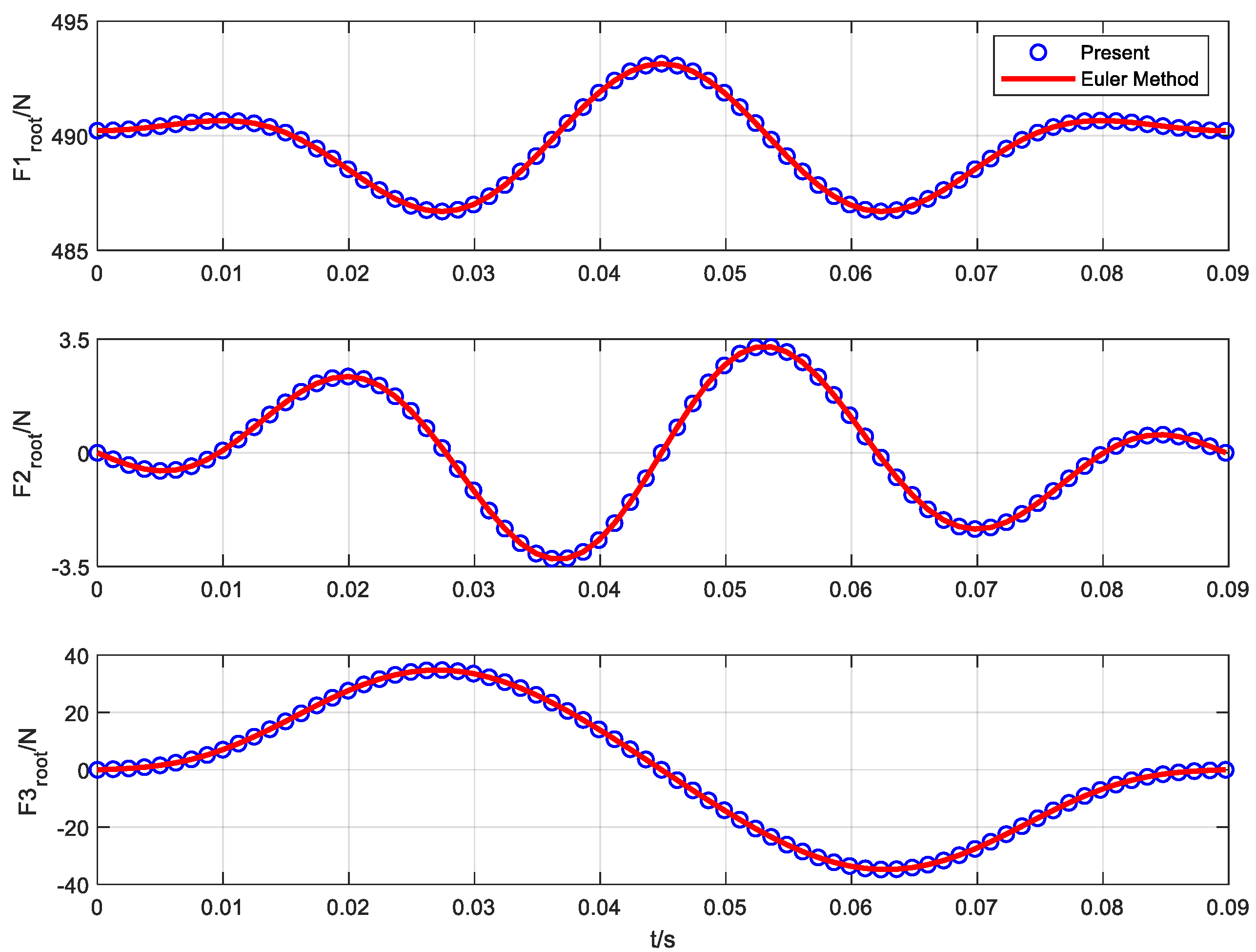
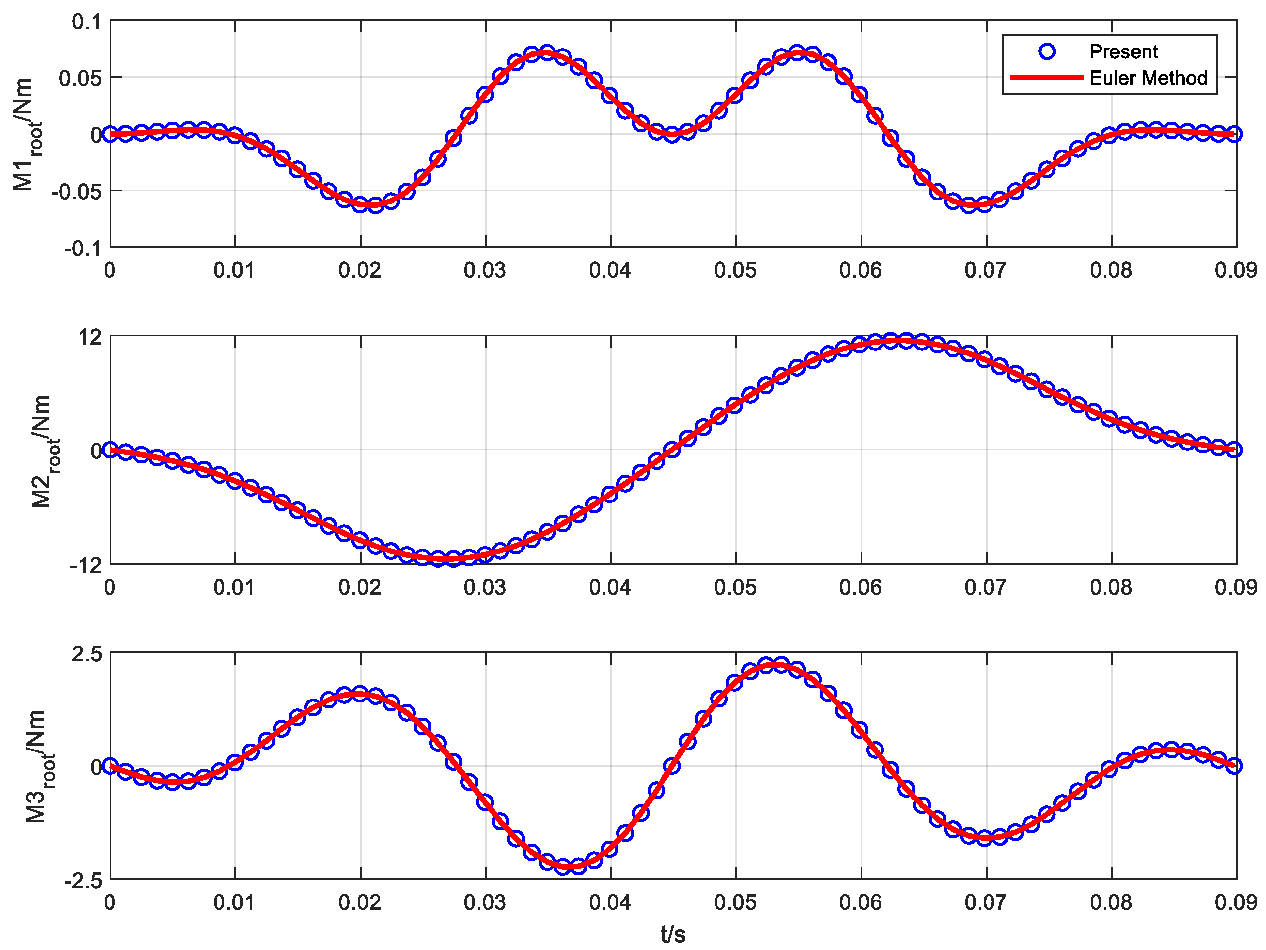
It can be seen in the matrix form that the coefficient matrix of the equations after dividing is characterized by a sparse banded distribution. Compared with the method of forming full matrix coefficients without dividing elements, the DQ−Pade element method can improve the calculation speed of the matrix and reduce the storage cost, thereby improving the calculation efficiency. The accuracy and efficiency of the method are verified by the following examples.

4. Numerical Results

To verify the applicability and validity of the proposed time/spatial discretization formula for intrinsic beam equations, two examples are considered. Firstly, the spatial discrete formula is verified by static analysis and modal calculation of the cantilever beam. Another example is calculating the dynamic response of a rotating cantilever beam to verify the accuracy and efficiency of the proposed time-discrete formula.

4.1. Static Analysis and Modal Calculation of the Cantilever Beam

Firstly, the static analysis of the following force applied to the tip of the cantilever beam is considered. Then, the velocity condition is applied to its root to calculate its natural frequency [10]. The structural characteristics of the cantilever beam are shown in Table 1. For static analysis, apply a following force F t i p = 3 E I / L 2 at the tip. Simitses and Hodges [34] gave the exact solution of the dimensionless equation (made by F t i p L ) for the bending moment at the root M ¯ r o o t = 0.8104403623 . Due to static analysis, time-dependent terms are eliminated in Equation (9), and it can be simplified to
k = 1 N W i k F k + κ ˜ i F i + W i L F L = 0 k = 1 N W i k M k + κ ˜ i M i + e ˜ 1 F i + W i L M L = 0
Table 2 lists the results of the root bending moment calculated by different DQ methods. The GDQ method is the discretization method based on Lagrange polynomial space that was used to calculate weight coefficients in [29]. The wavelet-differential quadrature (WDQ) method is a DQ method based on the adaptive multi-layer wavelet collocation method in [27,28]. The number of discrete points is determined by the wavelet resolution layer j and the translation factor N ( n = 2 j + 1 + 2 N + 1 ), and N = 2 , j = 0 4 is taken here. The results of the central difference method (CDM) used by the Hodges [4] are also listed in this table.
From Table 2 and Figure 3 and Figure 4, it can be clearly seen that the DQ methods has better accuracy than the CDM. Compared with the other two DQ methods, the DQ−Pade method has obvious advantages in convergence speed. With the same computational cost, the accuracy of this method is at least three orders of magnitude higher than those of the other two methods. To achieve the minimum error magnitude of 10−10, only nine discrete points are needed in this method. The computational cost is much lower than 16 points for the GDQ method and 37 points for the WDQ method.
However, it can be seen in Figure 3 that when the number of discrete points exceeds 9, the calculation accuracy of this method decreases as the number of discrete points increases. The reason is that with the increase in the number of discrete points, it will be difficult to calculate the distributed discrete points, resulting in a decrease in the accuracy of calculating discrete weight coefficients. Figure 4 shows the error curve of calculating the bending moment at the root by dividing different discrete element numbers. It can be seen in the figure that dividing discrete elements can effectively improve the calculation accuracy and restrain the divergence of error. At the same time, it is worth noting that as the number of element (M) increases, the rate of error convergence decreases. Additionally, it is observed that when the number of discrete points in single element exceeds 10, the accuracy usually decreases. Therefore, it is recommended to divide the sub-domains as little as possible in the entire domain, and discretize points in any sub-domain no more than 10 times.
If the intrinsic dynamic boundary conditions of the rotating cantilever beam [10] are
V 0 T = [ 0 , 51.03 , 0 ] , Ω 0 T = [ 0 , 0 , 3.189 ] , F L T = [ 0 , 0 , 0 ] , M L T = [ 0 , 0 , 0 ]
Wright [35] gave an exact solution for the bending frequency in this case:
ω 1 s t , b e n d i n g = 5.703 , ω 2 n d , b e n d i n g = 18.72 , ω 3 r d , b e n d i n g = 44.50
Table 3 lists the frequency results of CDM, DQ−Pade, and the GDQ method. The CDM is sensitive to the calculation step, so it needs more discrete points. It was found that the frequency results had considerable accuracy when the number of discrete points exceeds 150. Compared with the GDQ method, our method still has the prominent characteristics of low cost and high precision, so it is an ideal choice for the spatial discretization of the fully intrinsic equations.

4.2. Dynamic Response of the Rotating Beam

In the second example, the dynamic response analysis of rotating cantilever beam is considered, including transient and steady-state responses. The length of the beam is 1 m, and the rotational speed is 70 rad/s. The material properties of the beam are shown in Table 4 [32].
A periodic excitation force F = 50 sin ( 20 t )   N is applied in the flapping direction at the tip of the beam. The transient response results of DYMORE with a calculation step size of 0.001 s is given in [32]. This present method had the same calculation cost: 125 time elements and 8 time points in each element, denoted as M125−N8. Tip displacement, tip rotation angle, root force, and bending moment are shown in Figure 5, Figure 6, Figure 7 and Figure 8, respectively. From these figures, it can be seen that the present method is in good agreement with the calculation results of DYMORE. Even for axial forces with insufficient calculation accuracy in [32], this method can still achieve satisfactory accuracy.
With the same rotational speed, a periodic harmonic force is applied in the direction of tip flapping:
F = 10 sin ( 70 t ) + 5 sin ( 2 70 t ) + 2 sin ( 3 70 t )   N
The authors of [32] used the backward second-order Euler method to calculate the time domain response. We took the Euler method as a reference for the steady-state response. Figure 9, Figure 10, Figure 11 and Figure 12 shows the steady-state periodic response curves of tip displacements, rotations, root forces, and moments calculated by the two methods. In the figures, the steady-state period formula of the DQ−Pade element method uses a combination of eight time elements divided in one period and nine distribution points used in each element (M8−N9), both of which use the same time element step size, t = 2 π / 70 / 72 (one time element per 5°). It can be seen in the figures that the two curves basically coincide, and both can well meet the periodic condition. When the calculation step size is 5°, the Euler method required six periods, and it took 114 s, to reach the so-so periodic boundary condition (absolute error < 1). When calculating 15 cycles, which took 286 s, the periodic boundary value condition converged to the order of 10−2. The results of Euler method in the figures are given for this condition.
The steady-state periodic boundary value formula of the DQ−Pade method itself satisfies the periodic boundary conditions. At the same calculation cost, i.e., calculating 72 time discrete points in a cycle, the calculation accuracy and calculation time were compared, with different combinations of discrete element numbers and discrete point numbers (M × N = 72). Taking M36−N10 (one time element per 1°) as a reference, and taking the bending moment of the beam root as an example, Figure 13 shows the convergence of different combinations. It can be seen that the combination of fewer discrete elements and more discrete points distributed in each element can obtain the best accuracy. Table 5 gives the calculation times of different combinations. The combination with the best accuracy took the longest, but this was still far less than the calculation time of the Euler method. The reason is that each time discrete point has a state quantity that contains all the structural degrees of freedom, and the increase in discrete points in the time element leads to the multiplication of the matrix operation cost. Therefore, it is needed to make a balance between accuracy and computational efficiency.

5. Conclusions

In this paper, a new method based on the DQ−Pade method was proposed to solve the nonlinear fully intrinsic equations of geometrically exact beams. Starting from the spatial and temporal discretization of the fully intrinsic equations, the DQ−Pade method was used to re-deduce the spatial discretization equations of the fully intrinsic beam equations, and the static analysis and modal calculation of the beam were investigated. It was found that the accuracy and efficiency of this method are better than those of the traditional GDQ method. In terms of time discretization, a calculation formula of initial value and steady-state periodic boundary value is proposed, based on the DQ−Pade method. With the consideration of the efficiency and accuracy of the DQ−Pade method, the DQ−Pade element method was further proposed. The results show that the method is very effective, and it has outstanding performance in terms of accuracy and efficiency, which makes a good foundation for the subsequent rotor vibration load prediction and aeroelastic stability analysis.

Author Contributions

Conceptualization, L.C. and Y.L.; methodology, L.C.; validation, L.C.; formal analysis, L.C.; investigation, L.C.; writing—original draft preparation, L.C.; writing—review and editing, L.C. All authors have read and agreed to the published version of the manuscript.

Funding

This research received no external funding.

Institutional Review Board Statement

Not applicable.

Informed Consent Statement

Not applicable.

Data Availability Statement

Not applicable.

Conflicts of Interest

The authors declare no conflict of interest.

References

  1. Bauchau, O.A.; Kang, N.K. A Multibody Formulation for Helicopter Structural Dynamic Analysis. J. Am. Helicop. Soc. 1993, 38, 3–14. [Google Scholar] [CrossRef]
  2. Hodges, D.H. A Mixed Variational Formulation Based on Exact Intrinsic Equations for Dynamics of Moving Beams. Int. J. Solids Struct. 1990, 26, 1253–1273. [Google Scholar] [CrossRef]
  3. Hodges, D.H.; Shang, X.; Carlos, C. Finite Element Solution of Nonlinear Intrinsic Equations for Curved Composite Beams. J. Am. Helicop. Soc. 1996, 41, 313–321. [Google Scholar] [CrossRef]
  4. Hodges, D.H. Geometrically Exact, Intrinsic Theory for Dynamics of Curved and Twisted Anisotropic Beams. AIAA J. 2003, 41, 1131–1137. [Google Scholar] [CrossRef]
  5. Hodges, D.H. Nonlinear Composite Beam Theory; AIAA: Reston, VA, USA, 2006. [Google Scholar]
  6. Green, A.E.; Laws, N. A General Theory of Rods. Proceed. Royal Soc. London 1966, 293, 145–155. [Google Scholar]
  7. Hegemier, G.A.; Nair, S. A Nonlinear Dynamical Theory for Heterogeneous, Anisotropic, Elasticrods. AIAA J. 1977, 15, 8–15. [Google Scholar] [CrossRef]
  8. Palacious, R.; Cesnik, C.E.S. Structural Models for Flight Dynamic Analysis of Very Flexible Aircraft. In Proceedings of the AIAA/ASME/ASCE/AHS/ASC Structures, Structural Dynamics, and Materials Conference, California, PS, USA, 4–7 May 2009. [Google Scholar]
  9. Patil, M.J.; Hodges, D.H. Flight dynamics of highly flexible flying wings. J. Aircr. 2006, 43, 1790–1799. [Google Scholar] [CrossRef] [Green Version]
  10. Patil, M.J.; Althoff, M. Energy-consistent, Galerkin approach for the nonlinear dynamics of beams using intrinsic equations. J. Vib. Control 2011, 17, 1748–1758. [Google Scholar] [CrossRef] [Green Version]
  11. Patil, M.J.; Hodges, D.H. Variable-order finite elements for nonlinear, fully intrinsic beam equations. J. Mech. Mater. Struct. 2011, 6, 479–493. [Google Scholar] [CrossRef] [Green Version]
  12. Sotoudeh, Z.; Hodges, D.H. Incremental method for structural analysis of joined-wing aircraft. J. Aircr. 2011, 48, 1588–1601. [Google Scholar] [CrossRef]
  13. Sotoudeh, Z.; Hodges, D.H. Modeling Beams with Various Boundary Conditions Using Fully Intrinsic Equations. J. Appl. Mech. 2011, 78, 031010. [Google Scholar] [CrossRef]
  14. Khaneh Masjedi, P.; Ovesy, H.R. Chebyshev collocation method for static intrinsic equations of geometrically exact beams. Int. J. Solids Struct. 2015, 54, 183–191. [Google Scholar] [CrossRef]
  15. Khaneh Masjedi, P.; Ovesy, H.R. Large deflection analysis of geometrically exact spatial beams under conservative and nonconservative loads using intrinsic equations. Acta Mech. 2014, 226, 1689–1706. [Google Scholar] [CrossRef]
  16. Tashakorian, M.; Ghavanloo, E.; Fazelzadeh, S.A.; Hodges, D.H. Nonlocal fully intrinsic equations for free vibration of Euler–Bernoulli beams with constitutive boundary conditions. Acta Mech. 2018, 229, 3279–3292. [Google Scholar] [CrossRef]
  17. Im, B.; Cho, H.; Shin, S.J. Geometrically Exact Beam Analysis Based on the Exponential Map Finite Rotations. Int. J. Aero. Space Sci. 2020, 21, 153–162. [Google Scholar] [CrossRef]
  18. Bellman, R.; Casti, J. Differential quadrature and long-term integration. J. Math. Anal. Appl. 1971, 34, 235–238. [Google Scholar] [CrossRef] [Green Version]
  19. Bert, C.W.; Jang, S.K.; Striz, A.J. New methods for analyzing vibration of structural components. AIAA J. 1987, 25, 936–943. [Google Scholar]
  20. Shu, C.; Richards, B.E. Application of generalized differential quadrature to solve two-dimensional incompressible NavierStokes equations. Int. J. Numer. Methods Fluids 1992, 15, 791–798. [Google Scholar] [CrossRef]
  21. Shu, C.; Richard, B.E. Parallel simulation of incompressible viscous flows by generalized differential quadrature. Comput. Syst. Eng. 1992, 3, 271–281. [Google Scholar] [CrossRef]
  22. Vasilyev, O.V.; Sen, M.; Paolucci, S. A Wavelet Collocation Method for Solving Partial Differential Equations in a Finite Domain. J. Computat. Physics 1995, 120, 33–47. [Google Scholar] [CrossRef] [Green Version]
  23. Vasilyev, O.V.; Paolucci, S. A Dynamically Adaptive Multilevel Wavelet Collocation Method for Solving Partial Differential Equations in a Finite Domain. J. Computat. Physics 1996, 125, 498–512. [Google Scholar] [CrossRef] [Green Version]
  24. Vasilyev, O.V.; Sen, M. A Fast Adaption Wavelet Collocation Algorithm for Multidimensional PDEs. J. Computat. Physics 1997, 138, 16–65. [Google Scholar] [CrossRef]
  25. Chen, C.N. The development of irregular elements for differential quadrature element method steady-state heat conduction analysis. Comput. Methods Appl. Mech. Eng. 1999, 170, 1–14. [Google Scholar] [CrossRef]
  26. Wei, L.C.; Striz, A.G.; Bert, C.W. High-accuracy plane stress and plate elements in the quadrature element method. Int. J. Solids Struct. 2000, 37, 627–647. [Google Scholar]
  27. Fung, T.C. Solving initial value problems by differential quadrature method-part 1: First-order equations. Int. J. Numer. Methods Engine. 2001, 50, 1411–1427. [Google Scholar] [CrossRef]
  28. Fung, T.C. Solving initial value problems by differential quadrature method-part 2: Second-and higher- order equations. Int. J. Numer. Methods Engine. 2001, 50, 1429–1454. [Google Scholar] [CrossRef]
  29. Amoozgar, M.R.; Shahverdi, H. Analysis of Nonlinear Fully Intrinsic Equations of Geometrically Exact Beams Using Generalized Differential Quadrature Method. Acta Mechanica 2016, 227, 1265–1277. [Google Scholar] [CrossRef]
  30. Amoozgar, M.R.; Shahverdi, H. Dynamic instability of beams under tip follower forces using geometrically exact, fully intrinsic equations. Lat. Am. J. Solids Struct. 2016, 13, 3022–3038. [Google Scholar] [CrossRef] [Green Version]
  31. Amoozgar, M.R.; Shahverdi, H.; Nobari, A.S. Aeroelastic stability of hingeless rotor blades in hover using fully intrinsic equations. AIAA J. 2017, 55, 2450–2460. [Google Scholar] [CrossRef]
  32. Cheng, T. Structural dynamics modeling of helicopter blades for computational aeroelasticity. Doctoral dissertation, Massachusetts Institute of Technology, Cambridge, MA, USA, 2002. [Google Scholar]
  33. Borri, M. Helicopter rotor dynamics by finite element time approximation. Comput. Math. Appl. 1986, 12, 149–160. [Google Scholar] [CrossRef] [Green Version]
  34. Simitses, G.J.; Hodges, D.H. Fundamentals of Structural Stability; Butterworth-Heinemann: Oxford, UK, 2006. [Google Scholar]
  35. Wright, A.D.; Smith, C.E.; Thresher, R.W.; Wang, J.L.C. Vibration modes of centrifugally stiffened beams. J. Appl. Mech. 1982, 49, 197–202. [Google Scholar] [CrossRef]
Figure 1. Sketch map of beam before and after deformation.
Aerospace 09 00596 g001
Figure 2. Distribution of discrete points when N = 9.
Aerospace 09 00596 g002
Figure 3. The accuracy comparison of different DQ methods.
Aerospace 09 00596 g003
Figure 4. Precision of the DQ−Pade element method.
Aerospace 09 00596 g004
Figure 5. Displacements time history curve of the beam tip.
Aerospace 09 00596 g005
Figure 6. Rotation time history curve of the beam tip.
Aerospace 09 00596 g006
Figure 7. Time history curve of beam root forces.
Aerospace 09 00596 g007
Figure 8. Time history curve of beam root moments.
Aerospace 09 00596 g008
Figure 9. Steady−state periodic curves of beam tip displacements.
Aerospace 09 00596 g009
Figure 10. Steady−state period curve of beam tip rotations.
Aerospace 09 00596 g010
Figure 11. Steady−state periodic curve of beam root forces.
Aerospace 09 00596 g011
Figure 12. Steady−state periodic curve of beam root moments.
Aerospace 09 00596 g012
Figure 13. Beam root flapping moment curves with different combinations of discrete elements and points.
Aerospace 09 00596 g013
Table 1. The structural characteristics of the cantilever beam.
ParameterValue
Span16 m
Chord1 m
Mass density0.75 kg/m
Moment of inertia (50% chord)0.1 kg m
Spanwise elastic axis50% chord
Center of gravity50% chord
Bending rigidity2 × 104 Nm2
Torsional rigidity1 × 104 Nm2
Bending rigidity (chordwise)4 × 10⁶ Nm2
Shear/extensional rigidity
Table 2. Results of the root bending moment calculated by different DQ methods.
Methodn = 3n = 4n = 5n = 6n = 7
CDM0.7959437080.8041113470.8069423290.8082270740.808914563
GDQ0.6289131290.8485046510.8031003610.8097029450.810900600
WDQ----0.811791100
Present0.8067621710.8099244050.8104143630.8104379050.810440225
n = 8n = 9n = 10n = 13n = 21
0.8093247790.8095890800.8097693360.8100644420.810305505
0.8103791360.8104303500.8104454530.8104404130.810440363
-0.810440438-0.8104400870.810440342
0.8104403540.8104403620.8104403630.8104403560.812366715
Table 3. Results of a beam rotating at natural frequency.
Frequencyn = 5n = 6n = 7n = 8n = 9n = 10
1st bending/Present5.70245.70245.70245.70245.70245.7024
1st bending/GDQM5.69835.70275.70235.70245.70245.7024
1st bending/CDM6.54026.38416.27796.20056.14176.0953
2nd bending/Present18.722618.722918.722918.722918.722918.7229
2nd bending/GDQM18.705418.720818.722618.722818.722918.7229
2nd bending/ CDM19.728319.715519.665019.602119.537719.4790
3rd bending/Present44.700844.512244.499744.498544.498544.4985
3rd bending/GDQM42.306942.269944.458744.501244.498344.4984
3rd bending/CDM35.399339.370241.289142.368443.029143.4587
Table 4. Material properties of the beam.
ParameterValue
Mass per unit length0.2 kg/m
Moment   of   inertia   per   unit   length   I x x 10−4 kg·m
Moment   of   inertia   per   unit   length   I y y 10−6 kg·m
Moment   of   inertia   per   unit   length   I z z 10−4 kg·m
Extensional   rigidity   K 11 106 N
Shear   rigidity   K 22 1020 N
Shear   rigidity   K 33 1020 N
Torsional   rigidity   K 44 50 N·m2
Bending   rigidity   K 55 50 N·m2
Bending   rigidity   ( chordwise )   K 66 1000 N·m2
Table 5. The calculation times of different combinations of discrete elements and points.
M/N36/224/318/412/69/88/9
CPU Time23.01 s25.17 s28.84 s38.88 s53.66 s63.12 s
Publisher’s Note: MDPI stays neutral with regard to jurisdictional claims in published maps and institutional affiliations.

