Article

Trajectory-Tracking Controller Design of Rotorcraft Using an Adaptive Incremental-Backstepping Approach

Department of Aerospace Engineering, Konkuk University, Seoul 05029, Korea
*
Author to whom correspondence should be addressed.
Aerospace 2021, 8(9), 248; https://doi.org/10.3390/aerospace8090248
Submission received: 25 June 2021 / Revised: 27 August 2021 / Accepted: 2 September 2021 / Published: 4 September 2021
(This article belongs to the Section Aeronautics)

Abstract

:
This paper treats a robust adaptive trajectory-tracking control design for a rotorcraft using a high-fidelity math model subject to model uncertainties. In order to control the nonlinear rotorcraft model which shows strong inter-axis coupling and high nonlinearity, incremental backstepping approach with state-dependent control effectiveness matrix is utilized. Since the incremental backstepping control suffers from performance degradation in the presence of control matrix uncertainties due to change of flight conditions, control system robustness is improved by combining the least squares parameter estimator to estimate time varying uncertainties contained in the control effectiveness matrix. Also, by selecting a suitable gain set by investigating the error dynamics, a uniform trajectory-tracking performance over operational flight envelope of the rotorcraft is ensured without resorting to the conventional gain scheduling method. To evaluate the proposed controller, comparative results between IBSC and Adaptive IBSC are provided in this paper with sequential maneuvers from the ADS-33E-PRF. The proposed method shows improved tracking performance under variations in control effective matrix in the flight simulation. Robust and stable parameter estimation is also guaranteed due to the implementation of the DF-RLS algorithm for the least squares estimator.

1. Introduction

With recent advances in the flight control system (FCS) technology, enabling safe and reliable operation of the aircraft became a fundamental requirement for FCS design. However, many challenges arise when designing a safe and robust rotorcraft FCS due to its highly nonlinear and inherently unstable dynamics. Jinshuo [1] thoroughly investigated the flight control technology for large-scale helicopters and classified the current challenges in the rotorcraft FCS design into the following four areas: (1) complicated dynamic response, (2) multiple flight modes, (3) model uncertainties and (4) rapid varying and wide operating conditions. This paper mainly focuses on an effective solution of these issues in the design of the trajectory-tracking controller for the rotorcraft using the adaptive backstepping control design.
The conventional linear control design has been still widely used for the rotorcraft and representative successful applications can be found in its implementations on the JUH-60A [2] and AH-64D [3]. It commonly uses multiple models linearized around a set of trim points and applies the gain-scheduling strategy to cover the wide operating conditions. Also, the associated control laws are typically layered by the outer-guidance and inner-stabilization control loops for the trajectory-tracking control [4,5]. While this approach allows an independent design of each loop, the overall close-loop system performance should be rigorously evaluated through a series of ground simulations and flight tests. In addition, the inner loops which is typically structured to mainly improve the on-axis responses require extreme additional design workloads to reduce the inter-axis couplings with complex model uncertainties that cannot be adequately addressed in the linear-control design. Therefore, it can be said that the traditional linear-control techniques may have many limitations in solving the mentioned challenges currently faced in the rotorcraft trajectory-tracking control design.
In the past three decades, advanced nonlinear control techniques such as nonlinear dynamic inversion [6,7], backstepping [8,9,10,11] and sliding mode [12,13,14] alongside with the use of nonlinear models have also gained much attention. Among them, the backstepping control design (BSC) became widely used in rotorcrafts due to its flexibility and systematic design process. However, the fact that BSC is highly sensitive to external disturbances and model uncertainties became the major drawback of this approach. A highly accurate nonlinear rotorcraft model is also very difficult to obtain in practice because of the complex flap, lead-lag, and inflow dynamics. Regarding the aforenoted reasons, techniques such as sliding mode observer [15,16], Neural nets [17,18] have been incorporated into BSC to enhance the controller’s robustness under model uncertainties and disturbances. In recent years, the control design with the incremental approach such as the incremental nonlinear-dynamic inversion [19,20] and incremental BSC (IBSC) [21,22,23] have also proven to be robust against model uncertainties. These sensor-based incremental methods use only a control effectiveness model by replacing the rest of the model with the measured or estimated acceleration, thereby reducing the model dependency related to system dynamics. However, controllers with incremental framework remains still sensitive to uncertainties in the control effectiveness matrix (CEM). Using parameter estimators with online update laws to estimate such uncertainties, many of incremental controllers combined with adaptive techniques such as least-squares (LS) [21,24], tuning-function (TF) [21,22], immersion and invariance (I&I) [21,25], and radial basis function (RBF) [26] have been developed.
This paper seeks to incorporate the LS estimator into the IBSC design in order to estimate and compensate uncertainties in CEM, which are strongly influenced by flight condition variation. The most common and cost-effective way to estimate such time varying uncertainties is to use Exponential forgetting recursive least squares (EF-RLS) by discounting past information using a constant forgetting factor. One of the main shortcomings of the EF-RLS is that accurate and stable estimates are only ensured in a case when the persistent excitation condition is met. During low excitation of the system, the covariance matrix may increase without bound (known as “covariance blow-up”), and the estimates might diverge or drift from their true values. Such excitation may not be rich for rotorcraft application where there exists little dynamic information when the rotorcraft is in a steady flight like stabilized hover and unaccelerated level forward flight. Also, the performance of EF-RLS is often sensitive to a pre-selected forgetting factor which is typically chosen by a trial-and-error process.
Considering these issues, various techniques such as variable forgetting [27,28] and direction forgetting [29,30,31] are widely investigated. A variable forgetting technique developed by Fortescue [27] determines the forgetting factor at each time step based on the information content of the upcoming data. A direction forgetting algorithm forgets the past information selectively by a pre-defined direction, ensuring the boundedness of the covariance matrix. With rigorous investigations of relevant issues, this paper adopts the direction forgetting recursive least squares algorithm (DF-RLS) of Cao and Schwartz [31] to ensure a stable and robust estimation of the CEM.
For an efficient design of controller without resorting to the gain-scheduling strategy, the present paper thoroughly investigates the tracking error dynamics and selects a gain set which can guarantee a uniform trajectory-tracking performance over OFE of the rotorcraft. The main contributions of this paper can be summarized as follows (1) The design of an adaptive IBSC (AIBSC) using the LS-based parameter estimator, (2) its applications to the rotorcraft trajectory-tracking problem using the high-fidelity math model, (3) the proposal of the effective gain selection strategy uniformly applicable over OFE, and (4) the validation of the proposed control solutions using various rotorcrafts’ mission-task-elements (MTEs) over a wide range of operating conditions. The rest of the paper is organized as follows: In Section 2, the problem statement for the rotorcraft trajectory-tracking control is presented considering uncertainties in an incremental dynamic framework. In Section 3, the LS-based estimator with Direction forgetting technique is presented. In Section 4, the AIBSC design based on a certainty equivalence principle is presented with the stability proof for overall closed-loop system using the Lyapunov-based method. Results of numerical simulations with BO-105 high fidelity model are presented in Section 5 to show the effectiveness of the proposed method. Finally, conclusions are drawn in Section 6.

2. Dynamic Model with Uncertainties

2.1. Helicopter Motion Equation

The rotorcraft dynamics can be represented with the following Euler equation in the body-fixed frame, and the kinematics for the linear and angular velocities:
v ˙ = 1 m f b ω × v ω ˙ = J 1 ( m b ω × J ω ) v = T v r ˙ ω = T ω φ ˙
where:
v = ( u v w ) , ω = ( p q r ) , φ = ( ϕ θ ψ ) , r = ( x y z )
The mass and the moment-of-inertia matrix of the rotorcraft are denoted by m and J , respectively. The transformation matrices are expressed with the definition of c x = c o s   x and s x = s i n   x by:
T v = ( C θ C Ψ C θ S Ψ S θ S Φ S θ C Ψ C Φ S Ψ S Φ S θ S Ψ + C Φ C Ψ S Φ C θ C Φ S θ C Ψ + S Φ S Ψ C Φ S θ S Ψ S Φ C Ψ C Φ C θ ) , T w = ( 1 0 S θ 0 C Φ S Φ C θ 0 S Φ C Φ C θ )
The position and heading angle are typically prescribed for the trajectory-tracking problem and the dynamics for the associated states can be derived using Equation (2) as follows:
v ˙ = T v r ¨ + T ˙ v r ˙ ω ˙ = T ω φ ¨ + T ˙ ω φ ˙
r ¨ = T v 1 { f b ( T ω φ ˙ ) × ( T v r ˙ ) } T v 1 T ˙ v r ˙ φ ¨ = T ω 1 J 1 { m b ( T ω φ ˙ ) × ( J T ω φ ˙ ) } T ω 1 T ˙ ω φ ˙
The external forces f b   and moments m b are typically derived using the component-based modeling techniques for the rotorcraft [4,32]. As an example, f b can be represented by the sum of each contribution of the main rotor ( m r ), fuselage ( f u s ), stabilizer ( s t b ), tail rotor ( t r ), and gravity ( g r v ) forces as:
f b = f m r + f f u s + f s t b + f t r + f g r v
The pitch angles of the main and tail rotors are typically used for the control of a conventional helicopter. In such a case, the primary controls u p = ( δ 0 , δ 1 C , δ 1 S , δ T R ) T consist of the collective, lateral-cyclic, longitudinal-cyclic pitches of the main rotor, and the collective pitch of the tail rotor, respectively. These controls cause the flap, lead-lag, and feathering motions of the rotor, which directly affect the forces ( f m r , f t r ) and moments ( m m r , m t r ) produced by the rotors. The associated dynamics (flap and lead-lag), and the resultant rotor force and moment are typically derived by applying the blade-element method (BEM) for a high-fidelity math model and by numerically integrating the nonlinear aerodynamic loads along the blade radial position [32].
The high-fidelity models are generally nonaffine to the primary control u p and may suffer from a wide range of model uncertainties. The forces and moments generated by the rotor are directly affected by uncertainties in the mass, aerodynamic, and elastic properties of the rotor blade. In addition, the states associated with the inflow model are typically defined in an averaged sense and non-measurable, which may add the uncertainty in the math model. Considering the separated time scales in the rigid-body and rotor dynamic modes, the dynamic rotor-trim approach is commonly adopted to design the flight controller only with the rigid-body dynamics [33]. In such a case, the motion equation which can be represented by the 2nd order dynamics for x = ( x , y , z , ϕ , θ , ψ ) T is derived as:
x ¨ = f n ( x , x ˙ , u p ) + d m ( x , x ˙ , u p )
Here, the force f n for the nominal plant corresponds to the right-hand-side terms of Equation (5) with model uncertainties term d m .

2.2. Incremental Dynamics

The incremental dynamics corresponding to Equation (7) are derived from the reference dynamics x ¨ 0 = f 0 + d m 0 = f n ( x 0 , x ˙ 0 , u p 0 ) + d m ( x 0 , x ˙ 0 , u p 0 ) represented by the known or measured states x 0 = x ( t 0 ) and controls u p 0 = u p ( t 0 ) at the previous time step t 0 . The incremental dynamics corresponding to the next time t = t 0 + Δ t are derived using incremental states x = x 0 + Δ x and controls u p = u p 0 + Δ u p . Therefore, the force vector at t = t 0 + Δ t can be approximated using the first-order Taylor-series expansion where the approximated dynamics can be derived as:
x ¨ f 0 ( x 0 + Δ x , x ˙ 0 + Δ x ˙ , u p 0 + Δ u p ) + d ( x 0 + Δ x , x ˙ 0 + Δ x ˙ , u p 0 + Δ u p ) f 0 + d m 0 + F 0 ( Δ x Δ x ˙ ) + D 0 ( Δ x Δ x ˙ ) + G 0 Δ u p + H 0 Δ u p x ¨ + F 0 ( Δ x Δ x ˙ ) + D 0 ( Δ x Δ x ˙ ) + G 0 Δ u p + H 0 Δ u p f n ( x , x ˙ , u p ) f 0 + F 0 ( Δ x Δ x ˙ ) + G 0 Δ u p d m ( x , x ˙ , u p ) d m 0 + D 0 ( Δ x Δ x ˙ ) + H 0 Δ u p x = x 0 + Δ x ,   x ˙ = x ˙ 0 + Δ x ˙
where F 0 = f 0 / ( x , x ˙ ) is the system matrix and G 0 = f 0 / u p is the control effectiveness matrix (CEM). D 0 = d m 0 / ( x , x ˙ ) and H 0 = d m 0 / ( u p ) , each of which refers to uncertainties in the system matrix and CEM. Since the dynamics related to incremental states Δ x ,   Δ x ˙ do not change significantly when the control input is updated in the infinitesimally small-time increment Δ t   the related terms can be neglected. Thus, the incremental dynamics of the system is written as:
x ¨ x ¨ 0 + ( G 0 + H 0 ) Δ u p
At this point, it is worth mentioning the favorable properties of the above incremental dynamics. First, the dynamics becomes affine to controls. Thus, they can be straightforwardly used for the IBSC design. Secondly, only the measured or estimated acceleration x ¨ 0 and the uncertainties in the CEM mainly affect the stability of the system. Therefore, assuming that sensor measurements are exact, the matched uncertainties H 0 are contained only in the linearized CEM. It can be claimed that the adverse effect of uncertainties can be completely removed in the control design, once G 0 is accurately estimated, that is, H 0 0 . This is one of the important reasons why this paper selects the incremental dynamics for the rotorcraft trajectory-tracking control.
A successful implementation of IBSC design requires the accurate acceleration x ¨ 0 at the previous time step. The linear accelerations are typically measured by the accelerometers in the navigation system, whereas sensors to measure the angular acceleration are rarely found on the market. As an alternative, many prediction algorithms have been developed and successfully used in the literatures [34,35]. The 1st order backward-difference formulas (BDF) are the simplest one among them. It uses the measured angular velocities and applies the following formula to estimate the angular acceleration at t = t k :
ω ˙ k = 1 Δ t ( ω k ω k 1 )
The 5th order BDF may provide a highly oscillatory estimate when there exists a sharp change in the measured angular velocity. In addition, the filtering methods typically requires a math model to determine the filter coefficients. Therefore, they highly depend on a specific math model and cannot be generalized for other models. This paper adopts the 1st order BDF for the prediction of the required angular acceleration and predicts the linear accelerations with those computed during the simulation.

3. Least-Squares Estimator

The certainty-equivalence principle has been widely adopted in estimation-based adaptive control design. There it is assumed that the uncertainty is exactly identified before the controller is designed. Under this principle, the design of the identification module can easily be separated from that for the controller and diverse range of estimation techniques can be adapted. Successful applications of the LS-based design have been reported in adaptive controls for aircraft [21,24]. As previously mentioned, an accurate estimation of the CEM G 0 is crucial to enhance the control robustness to model uncertainties in the IBSC design. Since the exact system parameters of rotorcraft are nearly impossible to find due to the complexity of rotor dynamics, analytically calculated Jacobian matrix using finite differences is often used to approximate one.
Nevertheless, calculating Jacobian matrices at each time step implies a heavy computational load due to the complexity of a high-fidelity rotorcraft model and is nearly impossible to execute in practice since the incremental dynamics require a high control update rate. Often, multiple linearized models obtained at different trim points along the wide operating conditions are scheduled to avoid this issue. However, the scheduled matrices may not represent the system dynamics when the aircraft is in an aggressive maneuver since they are only valid around their trim points. For these purposes, this paper adopts the LS-based estimator to estimate such time varying system parameters and to avoid carrying heavy inboard model of a rotorcraft. System parameters in the flight dynamic society are typically defined using the Euler equation in Equation (1), which is represented in the aircraft body-fixed frame. Applying incremental dynamics in Euler equation in Equation (1) gives:
n ˙ n ˙ 0 + B Δ u p n = ( v ω ) , n ˙ = ( v ˙ ω ˙ ) B = ( B v B ω ) = ( v ˙ / u p J ω ˙ / u p )
where v ˙ 0 ,   ω ˙ 0 are obtained using the relationship of Equation (4) with x ¨ 0 . The unknown parameters corresponding to Equation (11) can be related to G 0 using Equation (3) as follows:
B 0 = ( T v 0 0 T ω ) 0 G 0 = T 0 G 0
The present LS estimator is designed to estimate B 0 . The matrices required for the implementation of AIBSC will be computed using G 0 = T 0 1 . If the subscript j is used for a time indicator like t = t j for the convenience of derivation, Equation (11) can be represented by the expression:
B j Δ u p , j n ˙ j n ˙ j 1 = c j
using the structured representation of B j = ( b j , 1 | b j , 2 | | b j , 4 ) . The estimation error in the incremental control forces of Equation (13) can be derived when all of c j are available as:
e j = Φ j b j c j
where the regressor matrix Φ j and the unknown parameter vector b j are:
Φ j = d i a g ( Δ n T , Δ n T , , Δ n T ) R 6 × 24 b j = ( b j , 1 b j , 2 b j , 3 b j , 4 ) T R 24 × 1
The estimation of b j should be accurate enough for control-design applications when they are predicted using the most recent data inasmuch as possible. For this purpose, the recursive LS estimator with the exponential forgetting algorithm (RLS-EF) is widely used to capture the time-varying natures of the unknown parameter. Considering the algorithmic features mentioned above, b j b ^ can be computed by the following well-known RLS-EF formulation using a constant forgetting factor λ :
b ^ k = b ^ k 1 + P k Φ k T ( c k Φ k b ^ k 1 ) P k 1 = λ P k 1 1 + Φ k T Φ k
However, one of the widely known disadvantages of the RLS-EF algorithm is that the regressor Φ has to be ‘persistently exciting (PE)’ to ensure stable estimation. Such assumption may not hold for aircraft application where there exists little dynamic information when the aircraft is in a steady flight or hover situation. With poor excitation of the system, the covariance matrix P may grow up to a large value leading to a “covariance blow-up” issue [36]. Thus, the estimation process becomes extremely sensitive to small disturbances and noises, leading to an inaccurate estimations. The property of stable estimation is of foremost importance to our research since the aircraft may be in a control failure if the estimated parameter diverges to a large value. To avoid such problem, the concept of “direction forgetting (DF)” has been widely studied in the field [29,30,31]. The basic concept of DF is to discount the covariance matrix only in the certain direction of the current excited data when the input data is rich. In this paper, we take the DF algorithm of Cao and Schwartz [31], which determines the forgetting direction based on the orthogonal decomposition of the information matrix R k = P k 1 along the excited data Φ k . The information matrix, R k is updated in the form of:
R k = R k , 1 + λ R k , 2 + Φ k T Φ k w h e r e R k , 1 Φ k T = 0 ,     R k , 2 Φ k T = R k Φ k T
where R k , 1 contains the information orthogonal to the excited data Φ k and R k , 2 contains part of the information matrix which is in the same parameter space of the current excitation. Equation (17) implies that forgetting is only applied to the part of covariance matrix R k , 2 , which is in the direction of the incoming data. By following the detailed derivations and proofs in [31], the covariance matrix can be bounded using the complete Directional Forgetting RLS (DF-RLS) shown as follows:
b ^ k = b ^ k 1 + P k Φ k T ( c k Φ k b ^ k 1 ) P k = P ¯ k ( Φ k P ¯ k Φ k T + I ) 1 P ¯ k Φ k T Φ k P ¯ k , j P - k = { P k 1 if   Φ k ε D F P k 1 + 1 λ λ ( Φ k P k 1 1 Φ k T ) 1 Φ k T Φ k if   Φ k > ε D F
where the dead zone ε D F is determined based on the noise level of the data.

4. Design of Incremental Backstepping Control Law

4.1. Incremental Backstepping Control

The IBSC control law will be designed based on the Lyapunov-function-based method using the dynamics shown in Equation (9). In a case when the position and heading of the aircraft is prescribed for the trajectory-tracking control, the corresponding system dynamics can be written as:
x ¨ x ¨ 0 + G 0 Δ u p y = ( x , y , z , ψ ) T
where the estimated parameter G 0   is obtained from Equation (12) and Equation (18). Since u p first appeared at the second differentiation y ¨ of the system output, Equation (19) has system dimensions of n = 12 , with its relative degree ρ r = 8 . Therefore, there exist four unobservable internal attitude dynamics for ( ϕ , ϕ ˙ , θ , θ ˙ ) . To effectively handle such an underactuated system, the slack-variable approach has been proposed by Kim [37] and Lee [38] to obtain the fully actuated form of the system dynamics. Thereby, the standard process for the iBSC design becomes applicable in an integrated manner by assuming that the trajectories for all internal states are known or designated a priori.
The fully actuated system dynamics corresponding to Equation (19) can be derived by adding the slack control matrix G s and the incremental stack variables Δ u s R 2 . Thereby formulating the system dynamics in an affine form of Δ u for convenience:
x ¨ = x ¨ 0 + G 0 Δ u + ξ y = x
where:
G 0 = ( G 0 , G s ) ξ = G s Δ u s Δ u = ( Δ u p Δ u s )
The control effectiveness matrix G s for the slack variables is typically chosen to get a well-conditioned square matrix for G 0 . In this paper, G s is simply designated by:
G s = ( 0 2 × 4 , I 2 × 2 , 0 2 × 1 ) T
The slack-variable vector ξ will be estimated to meet the Lyapunov stability criteria. Using their estimates ξ ^ , the corresponding errors ξ ˜ are related to the exact ones ξ . Assuming that ξ is slowly varying, the error dynamics can be expressed by:
ξ ˜ ˙ = ξ ^ ˙   using   ξ = ξ ^ + ξ ˜
As in the IBSC control design, the tracking errors in the position and velocity trajectories are defined using the pseudo control α as:
z 1 = x x d z 2 = x ˙ α
By differentiating Equation (24) the error dynamics are derived as:
z ˙ 1 = z 2 + α x ˙ d z ˙ 2 = x ¨ 0 + G 0 Δ u + ξ α ˙
The BSC design typically defined the controller structure using the recursive approach consisting of the sequential definition of the control Lyapunov function (CLF) and derivation of the corresponding stability conditions. In this paper, the integrated approach is adopted, and stability can be proved based on the following CLF V :
V = 1 2 z 1 T Q 1 z 1 + 1 2 z 2 T z 2 + 1 2 ξ ˜ T Γ ξ 1 ξ ˜
The weight matrices of Q , Γ ξ , and { Λ j } j = 1 j = N are positive definite and typically defined using the diagonal ones. The controller structure can be defined using the stability condition V ˙ 0 . Using Equation (25), V ˙ can be derived in detail as follows:
V ˙ = z 1 T Q 1 z ˙ 1 + z 2 T z ˙ 2 + ξ ˜ T Γ ξ 1 ξ ˜ ˙       = z 1 T Q 1 ( α x ˙ d ) + z 2 T ( Q 1 z 2 + x ¨ 0 + G 0 Δ u + ξ α ˙ ) + ξ ˜ T Γ ξ 1 ξ ˜ ˙
The control structure becomes definable by putting condition on V ˙ to become negative definite. Using Equation (28) with the parameter matrices of K 1 , K 2 > 0 , leads to:
α = Q K 1 z 1 + x ˙ d Δ u = G 0 1 ( x ¨ 0 + Q 1 z 2 + K 2 z 2 + ξ ^ α ˙ )
With:
V ˙ = z 1 T K 1 z 1 z 2 T K 2 z 2 + ξ ˜ T ( Γ ξ 1 ξ ˜ ˙ + z 2 )
Using Equation (29), the dynamics for the update of ξ ^ can be defined to obtain the final stability condition shown in Equation (30):
ξ ^ ˙ = Γ ξ z 2
V ˙ = z 1 T K 1 z 1 z 2 T K 2 z 2 0
The application of control law Equation (28) and updated Equation (30) satisfies the stability condition as proven in Equation (31). Hence, by Lyapunov stability theory, the system is globally asymptotically stable.

4.2. Tuning the Controller Gains

The gain tuning process of the proposed incremental backstepping controller may be a time-consuming task. In order to ensure high tracking performance over an entire flight region with a single gain, the gain selection method is derived in this section through tracking error dynamics. The error dynamics of z 1 can be obtained as follows:
z ¨ 1 = x ¨ x ¨ d = f + G 0 Δ u + d + ξ x ¨ d
By substituting Equation (32) with the control input in Equation (28), the error dynamics becomes:
z ¨ 1 = Q 1 z 1 K 2 ( z ˙ 1 + Q K 1 z 1 ) Q K 1 z ˙ 1 + ξ ˜
Rearranging it into a 2nd order ordinary difference equation gives:
z ¨ 1 + ( K 2 Q K 1 ) z ˙ 1 + ( K 2 Q K 1 + Q 1 ) z 1 = ξ ˜
Therefore, the control gains and weight matrices are directly related to the tracking performance of the controller. With the selected natural frequencies and damping ratio for each axis, the gains can be selected in the following manner:
k 2 j + q j k 1 j = 2 ζ j ω j k 2 j q j k 1 j + q j = ω j 2
Rearranging into an equation with each gain gives:
k 1 j = 1 q j ( ζ j ω j ± 1 q j ( 1 ζ j 2 ) ω j 2 )
k 2 j = ζ j ω j 1 q j ( 1 ζ j 2 ) ω j 2
Also, the range of gain q j is determined considering the range of damping ratio:
1 ω j 2 q j 1 ( 1 ζ j 2 ) ω j 2
The maximum value of Equation (38) is selected in this paper to avoid selecting the remaining gains by a near 0 value:
q j = ( ω j 2 ω j 2 ζ j 2 ) 1
Therefore, by selecting the gain according to Equation (37), one can reduce the design workloads and ensure that the desirable response characteristics of Equation (34) is uniformly met in the OFE:
k 1 j = ζ j ω j q j , k 2 j = ζ j ω j , q j = 1 ( 1 ζ j 2 ) ω j 2

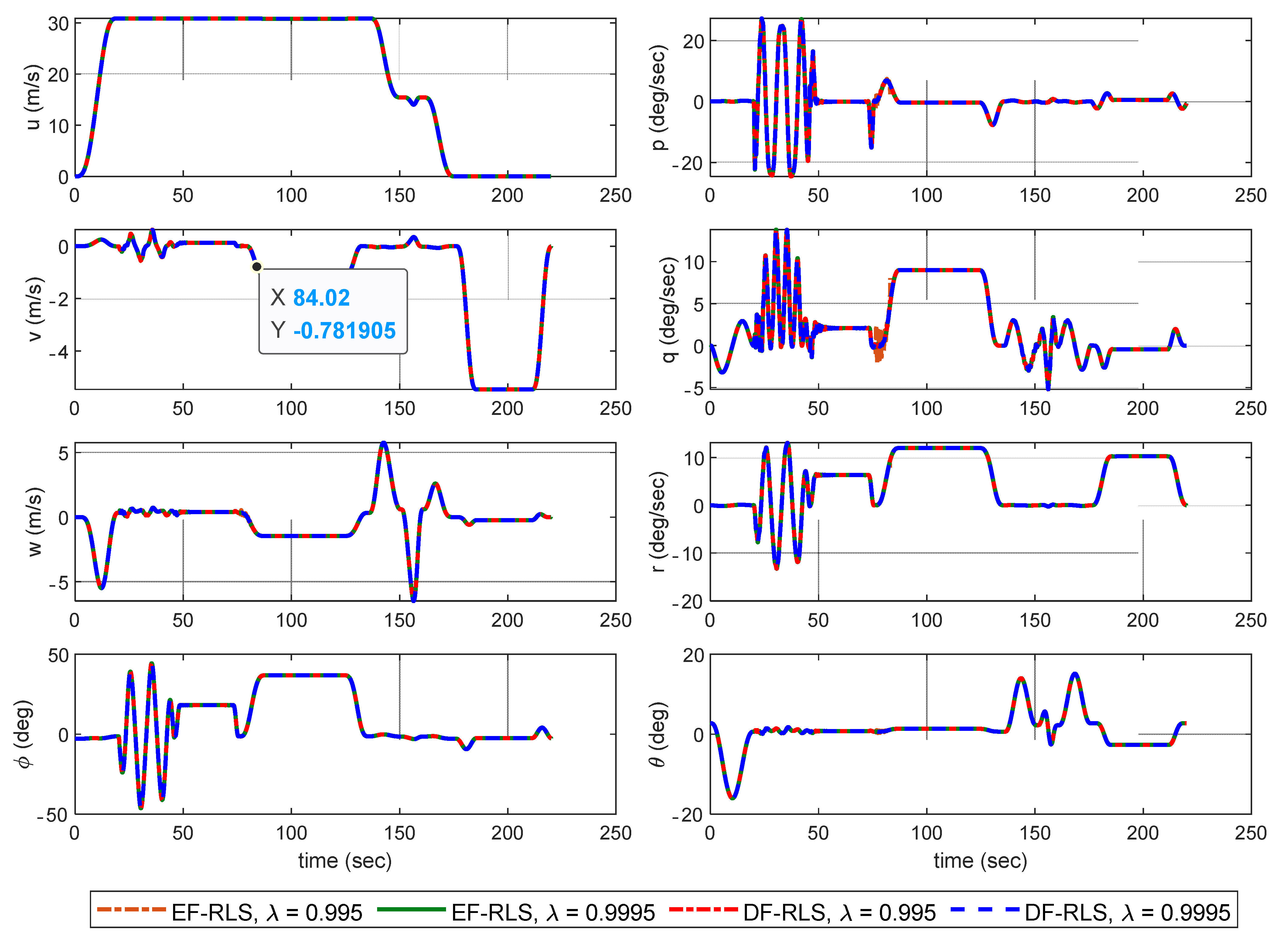
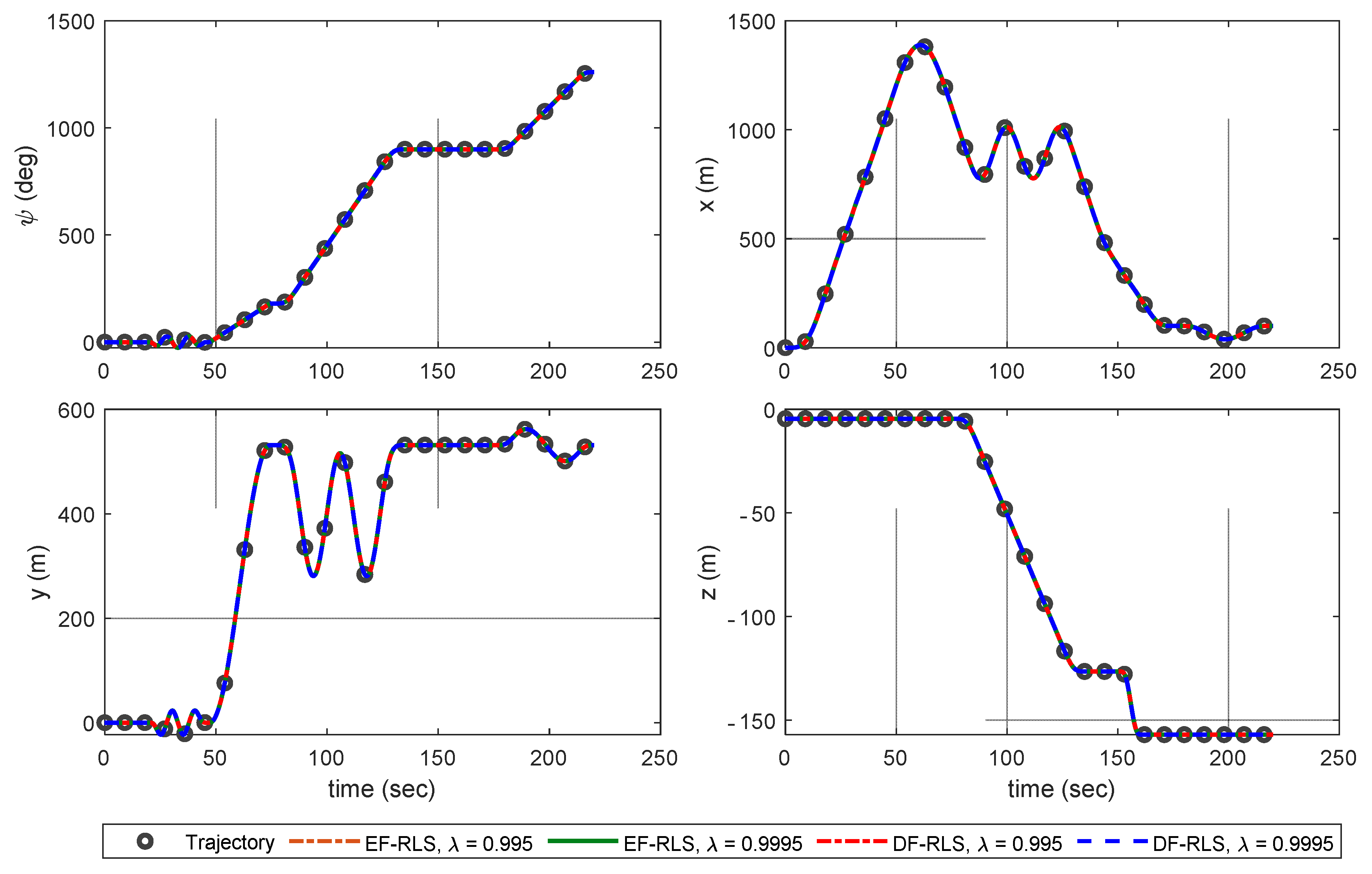
5. Applications and Discussions

Results of a numerical simulation will now be presented to validate the effectiveness of the proposed Adaptive Incremental backstepping controller. To show superior performance of the proposed method, trajectory tracking with: (1) incremental backstepping (IBSC) and (2) adaptive incremental backstepping (AIBSC), are performed. The highly fidelity flight dynamics model of a BO-105 from HETLAS [32] is used to simulate a sequence of maneuvers in ADS-33E-PRF [39]. The rotorcraft is initially trimmed at a steady-level flight condition with hovering condition at h = 100 ft. The flight simulation is conducted under a time step size of 0.001 s with the 4th order Runge-Kutta integrator. A control update rate of 100 Hz chosen in order to satisfy the underlying assumption of the incremental framework.
Reference trajectories are generated using the spline-trajectory generator. The trajectory consists of the following maneuvers. The rotorcraft initiates an acceleration maneuver up to 60 knots from the initial hover position. Then, a sequence of slalom, transient turn, and helical turn maneuver is performed at 60 knots and the rotorcraft decelerates to 30 knots. After performing pop-up maneuver the rotorcraft decelerate back to 0 knot and performs a pirouette maneuver. The summarized sequence of maneuvers is shown in Table 1.
During the maneuver, rotor trim solutions are used to eliminate the effect of high-frequency oscillatory forces and moments related to the rotor and inflow dynamics. The generated trajectories are shown in Figure 1, Figure 2 and Figure 3.
Here, simulations are conducted to validate the usefulness of the present method compared to the IBSC. For both controllers, the natural frequency and the damping ratio for gain selection are selected as ζ j = 0.75 and ω j = 2.0 uniformly for all axes. For parameter estimation, an initial covariance matrix is set as P 0 = 10 1 I with ε D F = 10 4 . Simulations with IBSC and AIBSC are performed in order to show increased performance of the proposed controller. First, Figure 4, Figure 5 and Figure 6 show simulations with various control effective matrices with IBSC. Each component of the control effective matrices b i , j are multiplied by a random constant factor α with normal distribution of zero mean in order to generate uncertainties within 10%, 20%, and 30% of its exact value. Simulation results are presented in Figure 4, Figure 5 and Figure 6.
b ^ i , j = ( 1 + α ) b i , j
From the results, one can see that system stability is not heavily affected within 20% inaccuracy of CEM. However, with 30% inaccuracy of CEM, the simulation showed severe control oscillations, particularly in aggressive maneuvers (slalom, transient turn and, helical turn). Although tracking performance is well maintained, even in the presence of control oscillations, such fluctuations are too severe for practical implementation on the actual rotorcraft. Also, in order to acquire exact CEM, finite differences must be used with a high-fidelity rotorcraft model which may burden the flight control computer with a heavy computational load. To show the improved robustness of AIBSC to uncertainties in CEM, simulations are performed with constantly updated control matrix using a LS-Estimator with DF-RLS algorithm and EF-RLS algorithm. Results are shown in Figure 7, Figure 8 and Figure 9.
The AIBSC shows superior tracking results without undesirable oscillatory control inputs The time varying control derivatives are constantly identified to make up for the instability resulting from the CEM mismatch. Figure 10 shows the estimation results of key control derivatives of CEM using: (1) EF-RLS and (2) DF-RLS, with different forgetting factors. The remaining control derivatives are omitted since their effectiveness is considerably small compared to the terms shown in Figure 10 or did not differ from their initial values throughout the simulation.
The dash-dotted black line in Figure 10 indicates the approximated control derivatives using finite differences from straight and level flight at hover to 60 knots. The results show that EF-RLS is highly sensitive to a selection of forgetting factor as in choosing λ = 0.995 in EF-RLS caused the estimates to diverge with an unstable closed loop stability and control failure in Figure 7. Since control input increments are rarely given ( Δ u p 0 ) in 50~75 s, that is, the persistent excitation condition is not met, the covariance matrix P grows without bound in EF-RLS. Thus, the estimator becomes extremely sensitive that estimates diverge even in the presence of small noises. One can see that the estimates did not diverge by choosing λ = 0.9995 in EF-RLS since the duration of stationary control inputs did not exceed the asymptotic memory length of the estimator. However, such condition may not hold in practical applications. This shows the main reason why DF-RLS is adopted in in this paper. The covariance matrix P remains bounded through direction forgetting technique, allowing the robustness of estimation to be guaranteed even when only poor control signals are given.
Pin-point accurate estimation of control derivatives was not guaranteed in some part of the flight envelope. The assumption that F 0 Δ x   and F 0 Δ x ˙ are left out in incremental dynamics of Equation (9) and the fact that angular accelerations are only a predicted value of the exact ones affect the estimation accuracy. The lack of persistently exciting signals also limits the estimator from converging to its true values although divergence of parameter is prevented through DF-RLS. Indirect adaptive controllers can be expected to misbehave, since such trajectories are obviously not persistently exciting in some maneuvers. To tackle this problem, robust control techniques can be additionally considered such as incremental backstepping sliding mode control to passively tolerate a wide range of model uncertainties [40]. Additional harmonic control inputs without regarding the tracking problem may also be considered [41]. In the latter case, additional excitation inputs must be preferably small to avoid losing track of desired trajectories. Examination between the tracking error and the magnitude of additional control inputs to ensure both accurate estimation and robust tracking performance remains as a further research. Nevertheless. Simulation results show that estimates are accurate enough to be used in the AIBSC controller to successfully track the desired trajectories. This is due to the property of IBSC that minor uncertainties in CEM does not heavily affect the stability of the system as in Figure 4, Figure 5 and Figure 6. Therefore, it can be claimed that the trajectory tracking of a helicopter can be successfully conducted in a wide range of flight envelope using AIBSC with the DF-RLS algorithm. The present design can be used to provide an excellent trajectory-tracking performance without depending on a heavy inboard flight model nor the complex calculation of the control Jacobian using a rotorcraft model.

6. Conclusions

This paper proposes an adaptive incremental backstepping controller for the trajectory tracking of a large-scale helicopter. With the incremental approach, the system dynamics can be shown in an affine from which is a combination of control effectiveness matrix and the acceleration measurements. Assuming that angular acceleration measurements are exact, only the CEM affects the control system stability. For a conventional fixed wing application, the system can straightforwardly be shown in a control affine form such as a fixed wing aircraft. Unfortunately, with the complex and nonlinear rotor dynamics of the helicopter, analytical solutions of the CEM cannot be easily obtained, and thus finite differences are used to estimate one. However, calculation of a control Jacobian using complex rotorcraft models during flight may impose a heavy computational burden on the flight computer. With the need of high sampling rate for the incremental dynamics, limitations may exist in practical applications.
To effectively identify the control effective matrix without the use of a computationally heavy inboard rotorcraft model, a certainty equivalence controller by incorporating the least squares parameter estimator is proposed. A simple and most common solution is to use the exponential forgetting recursive least squares method. Such a solution, however, causes any estimate to diverge when persistent excitation conditions are not met. That is, the robustness of the estimation was not guaranteed when the input signals are poor. A more attractive solutions is to use a direction forgetting technique which bounds the covariance matrix. The control method of integrating a direction forgetting based estimator and the incremental backstepping control update law for the rotorcraft trajectory control significantly improves the trajectory tracking performance and the response of the rotorcraft.
The gain selection process has also been incorporated to maintain uniform tracking performance along the flight and avoid conventional gain selection by trial and error. By constantly using estimated model parameters and a unified gain obtained through selection process, the proposed controller is uniformly applicable over the whole operational flight envelope without resorting to the conventional gain scheduling method. The validation of the proposed control solutions using various rotorcraft mission task elements from ADS-33E-PRF are shown in this paper.

Author Contributions

Conceptualization, U.J. and C.-J.K.; methodology, U.J.; software, U.J. and C.-J.K.; validation, U.J., M.-G.C. and C.-J.K.; formal analysis, U.J. and M.-G.C.; investigation, U.J.; resources, U.J. and J.-W.W.; data curation, U.J.; writing—original draft preparation, U.J.; writing—review and editing, U.J., M.-G.C. and C.-J.K.; visualization, U.J. and J.-W.W.; supervision, C.-J.K. All authors have read and agreed to the published version of the manuscript.

Funding

This research received no external funding.

Institutional Review Board Statement

Not applicable.

Informed Consent Statement

Not applicable.

Acknowledgments

This research was supported by Basic Science Research Program through the National Research Foundation of Korea (NRF) funded by the Ministry of Education (No. 2020R1A6A1A03046811). This work was supported by the National Research Foundation of Korea (NRF) grant funded by the Korea government (MSIT) (NRF-2020R1A2C2011955). This paper was written as part of Konkuk University’s research support program for its faculty on sabbatical leave in 2021.

Conflicts of Interest

The authors declare no conflict of interest.

References

  1. Hu, J.; Gu, H. Survey on Flight Control Technology for Large-Scale Helicopter. Int. J. Aerosp. Eng. 2017, 2017, 1–14. [Google Scholar] [CrossRef]
  2. Frost, C.R.; Hindson, W.S.; Moralez, E.; Tucker, G.E.; Dryfoos, J.B. Design and testing of flight control laws on the rascal research helicopter. In Proceedings of the AIAA Modelilng and Simulation Technologies Conference Exhibit, Monterey, CA, USA, 5–8 August 2002; pp. 1–11. [Google Scholar] [CrossRef]
  3. Harding, J.; Moody, S.J.; Jeram, G.J.; Mansur, M.H.; Tischler, M.B. Development of Modern Control Laws for the AH-64D in Hover/Low Speed Flight. In Proceedings of the 62nd Annual Forum of the American Helicopter Society, Phoenix, AZ, USA, 9–11 May 2006. [Google Scholar]
  4. Padfield, G.D. Helicopter Flight Dynamics; Blackwell: Oxford, UK, 2018; ISBN 9781405118170. [Google Scholar]
  5. Van Ekeren, W.; Looye, G.; Kuchar, R.; Chu, Q.; Van Kampen, E.J. Design, implementation and flight-test of incremental backstepping flight control laws. In Proceedings of the AIAA Guidance, Navigation, and Control Conference 2018, Kissimmee, FL, USA, 8–12 January 2018; pp. 1–21. [Google Scholar] [CrossRef]
  6. Ireland, M.L.; Vargas, A.; Anderson, D. A comparison of closed-loop performance of multirotor configurations using non-linear dynamic inversion control. Aerospace 2015, 2, 325–352. [Google Scholar] [CrossRef]
  7. Horn, J.F. Non-linear dynamic inversion control design for rotorcraft. Aerospace 2019, 6, 38. [Google Scholar] [CrossRef] [Green Version]
  8. Zou, Y.; Zheng, Z. A Robust Adaptive RBFNN Augmenting Backstepping Control Approach for a Model-Scaled Helicopter. IEEE Trans. Control Syst. Technol. 2015, 23, 2344–2352. [Google Scholar] [CrossRef]
  9. Xian, B.; Guo, J.; Zhang, Y. Adaptive backstepping tracking control of a 6-DOF unmanned helicopter. IEEE/CAA J. Autom. Sin. 2015, 2, 19–24. [Google Scholar] [CrossRef]
  10. Yan, K.; Wu, Q.; Chen, M. Robust adaptive backstepping control for unmanned autonomous helicopter with flapping dynamics. In Proceedings of the IEEE International Conference on Control and Automation (ICCA), Ohrid, Macedonia, 3–6 July 2017. [Google Scholar]
  11. Ahmed, M.; Subbarao, K. Target tracking in 3-D using estimation based nonlinear control laws for UAVs. Aerospace 2016, 3, 5. [Google Scholar] [CrossRef]
  12. Nafia, N.; El Kari, A.; Ayad, H.; Mjahed, M. Robust Full Tracking Control Design of Disturbed Quadrotor UAVs with Unknown Dynamics. Aerospace 2018, 5, 115. [Google Scholar] [CrossRef] [Green Version]
  13. Spurgeon, S.K.; Edwards, C.; Foster, N.P. Robust Model Reference Control Using a Sliding Mode Controller/Observer Scheme with Application to a Helicopter Problem. Available online: ieeexplore.ieee.org (accessed on 25 August 2021).
  14. McGeoch, D.J.; McGookin, E.W.; Houston, S.S. MIMO sliding mode attitude command flight control system for a helicopter. In Proceedings of the Collection of Technical Papers—AIAA Guidance, Navigation, and Control Conference, San Francisco, CA, USA, 15–18 August 2005; Volume 6. [Google Scholar]
  15. Madani, T.; Benallegue, A. Backstepping sliding mode control applied to a miniature quadrotor flying robot. In Proceedings of the IECON 2006—32nd Annual Conference on IEEE Industrial Electronics, Paris, France, 6–10 November 2006; pp. 700–705. [Google Scholar] [CrossRef]
  16. Madani, T.; Benallegue, A. Sliding mode observer and backstepping control for a quadrotor unmanned aerial vehicles. In Proceedings of the 2007 American Control Conference, New York, NY, USA, 9–13 July 2007; pp. 5887–5892. [Google Scholar] [CrossRef]
  17. Kwan, C.; Lewis, F.L. Robust backstepping control of nonlinear systems using neural networks. IEEE Trans. Syst. Man Cybern. Part A Syst. Humans 2000, 30, 753–766. [Google Scholar] [CrossRef]
  18. Lee, T.; Kim, Y. Nonlinear adaptive flight control using backstepping and neural networks controller. J. Guid. Control. Dyn. 2001, 24, 675–682. [Google Scholar] [CrossRef]
  19. Ji, C.H.; Kim, C.S.; Kim, B.S. A hybrid incremental nonlinear dynamic inversion control for improving flying qualities of asymmetric store configuration aircraft. Aerospace 2021, 8, 126. [Google Scholar] [CrossRef]
  20. Simplício, P. Helicopter Nonlinear Flight Control: An Acceleration Measurements-based Approach Using Nonlinear Dynamic Inversion. Control. Eng. Pract. 2011, 21, 1065–1077. [Google Scholar] [CrossRef]
  21. van Gils, P.; van Kampen, E.; de Visser, C.C.; Chu, Q.P. Adaptive incremental backstepping flight control for a high-performance aircraft with uncertainties. In Proceedings of the AIAA GuidanceNavigation, and Control Conference, San Diego, CA, USA, 4–8 January 2016. [Google Scholar] [CrossRef]
  22. Ignatyev, D.I.; Shin, H.S.; Tsourdos, A. Two-layer adaptive augmentation for incremental backstepping flight control of transport aircraft in uncertain conditions. Aerosp. Sci. Technol. 2020, 105, 106051. [Google Scholar] [CrossRef]
  23. Jeon, B.J.; Seo, M.G.; Shin, H.S.; Tsourdos, A. Understandings of the Incremental Backstepping Control Through Theoretical Analysis under the Model Uncertainties. In Proceedings of the 2018 IEEE Conference on Control Technology and Applications (CCTA), Copenhagen, Denmark, 21–24 August 2018; pp. 318–323. [Google Scholar] [CrossRef] [Green Version]
  24. Smeur, E.J.J.; Chu, Q.; De Croon, G.C.H.E. Adaptive incremental nonlinear dynamic inversion for attitude control of micro air vehicles. J. Guid. Control. Dyn. 2016, 39, 450–461. [Google Scholar] [CrossRef] [Green Version]
  25. Ali, A.A.H.; Chu, Q.P.; Van Kampen, E.; De Visser, C.C. Exploring adaptive incremental backstepping using immersion and invariance for an F-16 aircraft. In Proceedings of the AIAA Guidance, Navigation, and Control Conference, National Harbor, MD, USA, 13–17 January 2014. [Google Scholar] [CrossRef]
  26. Chang, J.; Guo, Z.; Cieslak, J.; Chen, W. Integrated guidance and control design for the hypersonic interceptor based on adaptive incremental backstepping technique. Aerosp. Sci. Technol. 2019, 89, 318–332. [Google Scholar] [CrossRef]
  27. Fortescue, T.R.; Kershenbaum, L.S.; Ydstie, B.E. Implementation of self-tuning regulators with variable forgetting factors. Automatica 1981, 17, 831–835. [Google Scholar] [CrossRef]
  28. Vaiopoulos, P.; Zogopoulos-Papaliakos, G.; Kyriakopoulos, K.J. Online Aerodynamic Model Identification on Small Fixed-Wing UAVs with Uncertain Flight Data. In Proceedings of the 2018 IEEE International Conference on Robotics and Automation (ICRA), Brisbane, Australia, 21–25 May 2018; pp. 6587–6592. [Google Scholar] [CrossRef]
  29. Campbell, S.F.; Nguyen, N.T.; Kaneshige, J.; Krishnakumar, K. Parameter estimation for a hybrid adaptive flight controller. In Proceedings of the AIAA Infotech@Aerospace Conference, Seattle, WA, USA, 6–9 April 2009; pp. 1–28. [Google Scholar] [CrossRef] [Green Version]
  30. Bittanti, S.; Bolzern, P.; Campi, M. Convergence and exponential convergence of identification algorithms with directional forgetting factor. Automatica 1990, 26, 929–932. [Google Scholar] [CrossRef]
  31. Cao, L.; Schwartz, H. Directional forgetting algorithm based on the decomposition of the information matrix. Automatica 2000, 36, 1725–1731. [Google Scholar] [CrossRef]
  32. Yun, Y.-H.; Kim, C.-J.; Shin, K.-C.; Yang, C.-D.; Cho, I.-J. Building the Flight Dynamic Analysis Program, HETLAS, for the Development of Helicopter FBW System. In Proceedings of the 1st Asian Australian Rotorcraft Forum and Exhibition 2012, Busan, Korea, 12–15 February 2012; pp. 12–15. [Google Scholar]
  33. Yang, C.-D.; Kim, C.-J.; Yang, S.-S. Rotorcraft Waypoint Guidance Design Using SDRE Controller. Int. J. Aeronaut. Space Sci. 2009, 10, 12–22. [Google Scholar] [CrossRef]
  34. Ovaska, S.J.; Väliviita, S. Angular acceleration measurement: A review. IEEE Trans. Instrum. Meas. 1998, 47, 1211–1217. [Google Scholar] [CrossRef]
  35. Han, J.D.; He, Y.Q.; Xu, W.L. Angular acceleration estimation and feedback control: An experimental investigation. Mechatronics 2007, 17, 524–532. [Google Scholar] [CrossRef] [Green Version]
  36. Åström, K.J.; Wittenmark, B. Adaptive Control, 2nd ed.; Addison-Wesley: Boston, MA, USA, 1995. [Google Scholar]
  37. Kim, M.; Kim, Y.; Jun, J. Adaptive sliding mode control using slack variables for affine underactuated systems. In Proceedings of the 2012 IEEE 51st IEEE Conference on Decision and Control (CDC), Maui, HI, USA, 10–13 December 2012; pp. 6090–6095. [Google Scholar] [CrossRef]
  38. Lee, D.; Kim, H.J.; Sastry, S. Feedback linearization vs. adaptive sliding mode control for a quadrotor helicopter. Int. J. Control Autom. Syst. 2009, 7, 419–428. [Google Scholar] [CrossRef]
  39. Baskett, B.J. Aeronautical Design Standard Performance Specification Handling Qualities Requirements for Military Rotorcraft; ADS-33E-PRF; US Army Aviation and Missile Command: Redstone Arsenal, AL, USA, 2000. [Google Scholar]
  40. Wang, X.; van Kampen, E.J. Incremental backstepping sliding mode fault-tolerant flight control. In Proceedings of the AIAA Scitech 2019 Forum, San Diego, CA, USA, 7–11 January 2019; pp. 1–23. [Google Scholar] [CrossRef]
  41. Morelli, E.A. Multiple input design for real-time parameter estimation in the frequency domain. IFAC Proc. Vol. 2003, 36, 639–644. [Google Scholar] [CrossRef] [Green Version]
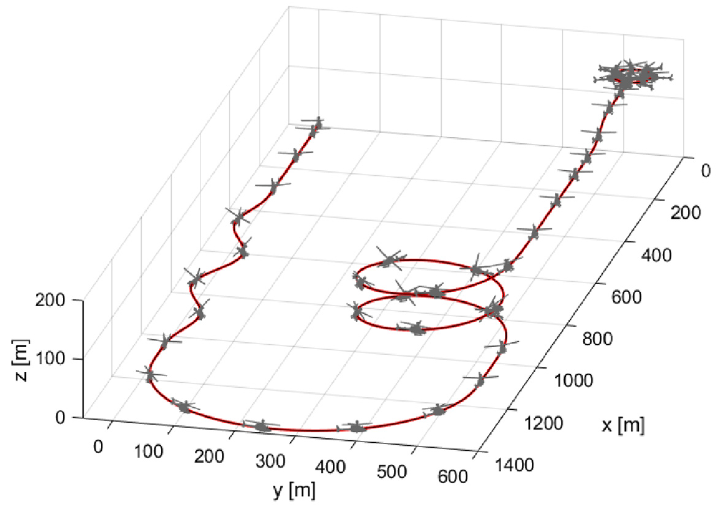
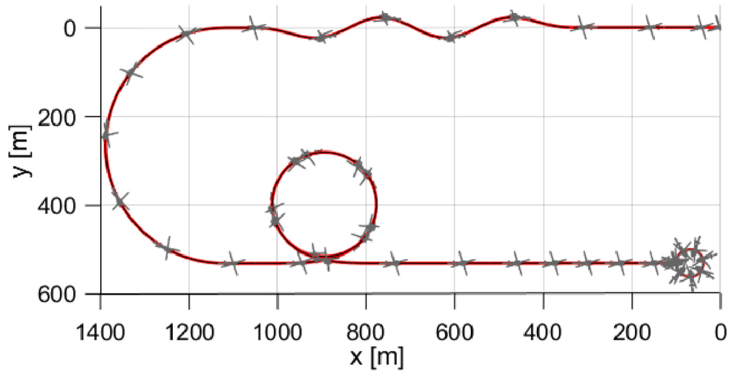
Figure 1. Trajectories for combined maneuver. Manoeuvers are selected from ADS-33E-PRF and are slightly edited.
Aerospace 08 00248 g001
Figure 2. Trajectories for combined maneuver. (Upper View).
Aerospace 08 00248 g002
Figure 3. Generated desired trajectories from spline trajectory generator: (a) velocity terms; (b) acceleration terms.
Aerospace 08 00248 g003
Figure 4. Simulation results of the trajectory tracking control with IBSC–Aircraft States.
Aerospace 08 00248 g004
Figure 5. Simulation results of the trajectory tracking control with IBSC-Control Inputs.
Aerospace 08 00248 g005
Figure 6. Simulation results of the trajectory tracking control with IBSC–Trajectory States.
Aerospace 08 00248 g006
Figure 7. Simulation results of the trajectory tracking control with AIBSC–Aircraft States.
Aerospace 08 00248 g007
Figure 8. Simulation results of the trajectory tracking control with AIBSC-Control Inputs.
Aerospace 08 00248 g008
Figure 9. Simulation results of the trajectory tracking control with AIBSC–Trajectory States.
Aerospace 08 00248 g009
Figure 10. Estimation results of key control derivatives.
Aerospace 08 00248 g010
Table 1. Maneuver specification for trajectory tracking.
ManeuversTime Length (s)Velocity Range (kts)Notes
Initial Condition0HoverInitial Height: 100 ft
Acceleration0~200 to 60/
Slalom20~4560/
Transient Turn45~7560180 deg turn
Helical Turn75~13560720 deg turn
Deceleration135~15060~30/
Pop up150~16030100ft ascent
Deceleration160~17530~0/
Pirouette175~2200Radius: 100 ft
Publisher’s Note: MDPI stays neutral with regard to jurisdictional claims in published maps and institutional affiliations.

