1. Introduction
Space debris is a threat to the safe operation of satellites and the long-term sustainability of space activities. The generation of space debris via collisions and explosions in orbit could lead to an exponential increase in the number of artificial objects in space in a chain reaction known as Kessler Syndrome [
1]. Nowadays, among the more than 8700 objects larger than 10 cm in Earth orbits, only about 6% are operational satellites, whereas the remainder is space debris. In addition, there are many smaller objects that are not routinely tracked, with estimates for the number of objects larger than 1 cm ranging from 100,000 to 200,000 [
2] and an estimated 128 million particles between 1 mm and 1 cm [
3]. Fragments of 1 cm size are particularly critical since they are very hard to detect, even in lower orbits, but can be mission-ending for operating satellites due to their high speed and, consequently, associated impact energy.
The dominant source of space debris by number of objects are breakup events, mainly due to on-orbit explosions and collisions. There are several reasons for breakup events, labelled by ESA Database and Information System Characterising Objects in Space (DISCOS) as follows [
4]: (i) propulsion: stored energy for non-passivated propulsion-related subsystems might lead to an explosion, for example due to thermal stress; (ii) upper stages explosions due to residual propellants; (iii) ullage motors; (iv) electrical: overcharging and subsequent explosion of batteries; (v) aerodynamics: breakup most often caused by an overpressure due to atmospheric drag; (vi) collision between two objects called
parents, usually referred to as
target (i.e., the primary or larger object) and
projectile (i.e., the secondary or smaller object); (vii) deliberate: intentional breakup events; (viii) anti-satellite tests (ASAT); (ix) anomalous: defined as “the unplanned separation, usually at low velocity, of one or more detectable objects from a satellite that remains essentially intact”.
Some of the events result in only a few objects, which might even quickly decay due to the atmospheric drag. In all the other cases, a large quantity of fragments is generated, thus significantly contributing to the increase in the collision risk that satellites are facing during their operational life [
4]. While implementing debris mitigation policies, space agencies and academia continuously develop models and software to analyze the space environment, estimating the collision probability between catalogued space objects and predicting future growth of debris population [
2,
3,
4,
5,
6,
7,
8,
9,
10,
11].
A fundamental component of any orbital debris environment evolution model is the satellite breakup model. The worldwide reference is the NASA Standard Breakup Model (SBM) implemented both in EVOLVE 4.0 [
12] and later in LEGEND [
9]. It provides three fundamental outputs: fragment size, area-to-mass ratio (
A/M), and relative velocity (Δ
V) distributions [
13]. Such distributions were obtained by a broad variety of data coming from deliberate hypervelocity collisions in Low Earth Orbit (LEO), ground-based impacts, and upper stage explosion tests, as well as from an extensive compilation of historical orbital data (i.e., TLE sets) for debris generated by explosions and collisions [
12].
Due to the semiempirical and statistical nature of the SBM, there are two major research paths concerning breakup models. On the one hand, there is the need to continuously update the list of catalogued space objects to have better data fitting. For this reason, a major effort made by different players in the space industry was to track and image space objects down to 1 cm at altitudes up to 1000 km, and down to 2 mm at low LEO altitudes [
2] thanks to the development of high performance ground-based RADAR systems (e.g., Space Fence, Haystack, TIRA, LeoLabs) [
14,
15,
16]. Moreover, other works aim to improve collision modelling via tests on new generation satellites, as a clear trend can be seen towards smaller and lower mass spacecraft [
17]. Simulations on Cosmos 2251-Iridium 33 collision and Fengyun-1C ASAT test demonstrated that while Cosmos 2251 fragments are well-described by the NASA SBM, noticeable discrepancies exist between the model predictions and the observation data for the Iridium 33 satellite and Fengyun-1C ASAT. The justification is that Cosmos 2251 was an older satellite while Iridium 33 and the Fengyun-1C weather satellites were relatively modern [
13,
18,
19]. Hence, NASA DebriSat project aims to characterize fragments generated by hypervelocity collisions involving a modern satellite in LEO. There are three phases to this project: the design and fabrication of DebriSat—an engineering model representing a modern, 60 cm/50 kg class LEO satellite; conduction of a laboratory-based hypervelocity impact to catastrophically break up the satellite, and characterization of the properties of breakup fragments down to 2 mm in size [
13,
18,
19]. Similarly, other experiments were carried out to characterize micro-satellite impacts (20 cm/1.5 kg), both at hyper and low velocity, varying impact directions and investigating fragments from multilayer insulation and solar cells [
20,
21]. Such experiments demonstrated that, although the SBM well represents the size distribution, mass and
A/M distributions are greatly influenced by the materials adopted [
20,
21].
Other software programs like IMPACT [
22,
23] introduce other inputs in the breakup model to better characterize the physical properties distribution of the fragments: the type of object (i.e., hollow or compact), the material density or, in case of explosion, the amount of energy driving the explosion (e.g., chemical energy, pressure, electrical energy). Moreover, while in the SBM the standard condition for a complete fragmentation is that the kinetic energy of the projectile relative to the target divided by the target mass is greater than 40 J/g, IMPACT introduces a further value of 10 J/g to smooth the transition from a typical hypervelocity collision with large numbers of small fragments to lower energy collisions where most of the target object is broken into a few larger fragments [
24].
The second research area regards the estimation of the input data of the SBM to model real fragmentation events. In the case of collisions, the input data are the mass of the two colliding objects,
M1 and
M2, and the impact velocity
vimp (i.e., the norm of the relative velocity). In the case of explosions, instead, an important role is played by the scale factor of the SBM, assuming a default value of 1 for upper stages with mass between 600 kg and 1000 kg [
12]. Several works [
4,
25,
26,
27], however, demonstrated that, giving such inputs, the number and the characteristics of the simulated fragments are different to the ones generated by a real breakup event. In particular, Anz–Meador and Matney [
25] and Braun et al. [
4] demonstrated that several debris clouds derived from explosions of nominal upper stages are represented by values of the scale factor significantly different from 1. Similarly, Pardini and Anselmo [
27] show that out of four on-orbit accidental collisions, all having an energy-to-mass ratio greater than 40 J/g, only one generated a number of fragments similar to the one predicted by the SBM. The reason is that the breakup model is purely energy-based and does not consider the relative attitude between the two colliding objects nor the point of collision. Indeed, the basic implementation of the SBM assumes that collisions will always involve the entire body of each parent. This does not account for spacecraft consisting of multiple connected structures; for instance, the presence of appendages such as gravity gradient booms or deployed solar panels. In this respect, the effect of a collision is clearly different if the projectile hits the main body of a satellite or only a part of it. In the latter case, the fragmented mass of the two objects will be probably lower and the breakup model would overestimate the number of the debris produced. Similarly, for explosions, the uncertainty regards the energy driving the breakup and, hence, the actual exploded mass. Therefore, a good estimation of the fragmented masses of the parents is critical to correctly set the input parameters of the SBM.
For the estimation of the scale factor, a simple procedure can be adopted as in [
28]: assuming that a certain number of fragments (
N*) over a minimum trackable size was catalogued, the scale factor can be derived explicitly from the equation of the cumulative distribution of the number of fragments with respect to the characteristic length. Another approach proposed by [
4] can be applied to both explosion and collision events. It consists of a dynamic scaling approach using a reported number of observed fragments (or number of catalogued fragments) multiplied by an altitude dependent catalogue incompleteness factor (so-called Henize factor) to scale the power law distribution. This procedure is used by [
4] to estimate the scale factor for explosions and the total fragmented mass of the parents for collisions. The Henize factor however presents a strong discontinuity for
Lc equal to 6 cm.
In this framework, this paper proposes an alternative way to estimate the tuning parameters for the SBM, focusing on the fragmented mass of the parents in case of collisions. The method requires TLE sets from the event to be analyzed. It assumes that enough time from the fragmentation event passed to have all the fragments over a certain size threshold catalogued. Moreover, decayed fragments are estimated. Hence, the breakup model is iterated until the number of simulated fragments over a predefined threshold of the characteristic length is equal to the number of real fragments, within a certain tolerance. The iteration is performed on the masses of the two parents separately after identifying the debris clouds derived from the target and the projectile. Finally, the fragmented masses of the parents are estimated using the bisection method.
An important assumption in this paper is that the parents and their orbits are known. However, a correct parent identification is not always guaranteed, thus leading to erroneously assigned objects. Several works proposed methods to identify the epoch of a fragmentation as well as the known objects involved. In particular, Frey et al. [
29,
30] propose a method to detect past fragmentations exploiting the convergence of mean Keplerian elements when propagating backwards in time. Tetrault et al. [
31] developed a tool that determines the objects involved in the fragmentation event using back propagation and particle distribution techniques. Dimare et al. [
32], instead, define a similarity function between the orbital elements of the objects under examination to establish a metric for the identification of the fragmentation. The parent objects are found by locating the minimum of the similarity function among the various objects. Romano et al. [
33] use backward propagation, pruning, and clustering algorithms to identify possible orbital intersection windows that make close encounters between objects possible. To consider erroneous assignment of the fragments to the parents, an analysis of the method performance under this circumstance is also carried out.
The remaining of the paper is organized as follows.
Section 2 provides a review of the Standard Breakup Model.
Section 3 describes the architecture of the SBM as implemented in this paper, focusing on the iterative approach.
Section 4 shows the test cases and the results obtained.
Section 5 draws some conclusions on the work presented and proposes future works.
2. Review of the Standard Breakup Model
The SBM models the fragment size,
A/M, and Δ
V distributions characterizing the debris generated by a fragmentation event [
13]. In this section, a synthetic description of the SBM, as implemented in EVOLVE 4.0, is reported. For more details regarding the derivation of the equations and the coefficients used in the statistical distributions, interested readers can refer to [
12].
The SBM identifies two types of fragmentation events: collisions and explosions. In case of collisions, the input data are the masses of the parents (i.e., the two colliding space objects) and the impact velocity. According to the model, collisions can be either
catastrophic if the entire masses of the two objects are fully fragmented or
non-catastrophic in case of fragmentation of the projectile and cratering of the target. The distinction between
catastrophic and
non-catastrophic collisions can be done by evaluating the relative kinetic energy of the projectile divided by the mass of the target, as shown below.
where
mtarg and
mproj are the masses of the target and projectile, respectively, while
vimp is the impact velocity. Specifically, the collision is defined as
catastrophic if the value of
Ep is greater than 40 J/g. In the case of
non-catastrophic collisions, i.e.,
Ep is less than 40 J/g, the fragmented mass of the parents is computed as follows [
12],
where
m1 and
m2 are the fragmented masses of the target and the projectile, respectively.
In the case of explosions, instead, the input data are the mass of the parent and a scale factor that has a unitary value for upper stages with a mass between 600 kg and 1000 kg.
The cumulative distribution of the number of fragments with respect to the characteristic length
Lc, is estimated using Equation (4) for collisions and Equation (5) for explosions.
where
N is the number of fragments,
mfrag is the fragmented mass, and
s is the scale factor. Then, the distribution of the number of fragments with respect to the
A/M, for each characteristic length interval, is computed. For each pair of
Lc-A/M intervals, values of characteristic length and area/mass ratio are extracted and then assigned to each fragment. It is assumed that within each interval there is a uniform probability distribution. The value of the area (
A) for each fragment is computed as a function of its length
Lc, using the following equation, valid both for collisions and explosions.
The mass value
M of each fragment can then be estimated as follows.
Finally, the distribution of the speed variations (ΔV) due to the event is computed and a ΔV value is assigned to each fragment by random extraction.
3. Breakup Model Sensitivity Analysis and Tuning Approach
The input data of the collision model are the masses of the parents and the impact velocity. The impact velocity (
vimp), normally computed from the state vectors of the parents, generally affects the fragmented mass during a collision. However, considering that the typical uncertainty in the knowledge of the impact velocity is in the order of m/s [
34], this effect is very limited. Moreover, as long as the number of catalogued fragments is known, the impact velocity does not influence the iterative estimation of the fragmented mass but its computational cost. In fact,
vimp is used only for the computation of the specific kinetic energy and, hence, for the definition of the type of collision (i.e., catastrophic or non-catastrophic). Such definition determines the initial values with which the iterative algorithm starts. Therefore, the impact velocity does not affect the final value of the estimated fragmented masses but only the number of iterations needed to reach convergence. In particular, if the collision is catastrophic, the impact velocity has no effect on the number of iterations, since the initial value of the iterative approach would always be equal to the total mass of the parents, regardless of the value of
vimp. In case of a non-catastrophic collision, the impact velocity instead enters directly in Equations (2) and (3) to compute the estimated fragmented mass according to the SBM. This could lead to an increase of number of iterations, e.g., from 2 to 5. Based on these considerations, the masses of the parents are the only parameters to tune the model. The tuning of the masses can be done based on the accurate information provided by the catalogued fragments: namely, their number and orbital parameters. The orbital parameters available for the catalogued fragments can provide useful information on the Δ
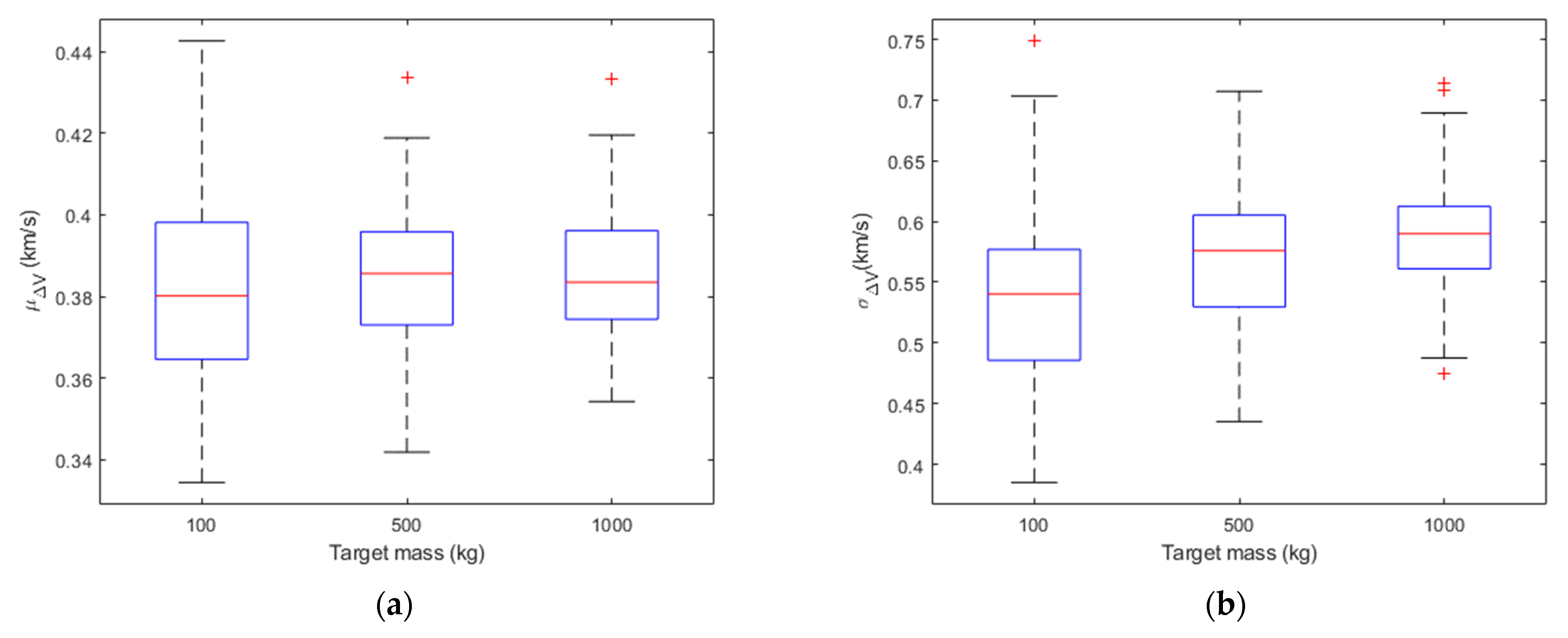
V distribution. However, such distribution seems to be rather insensitive to the input masses. To support this statement, a sensitivity analysis was carried out. For a fixed value of the projectile mass, set equal to 100 kg, the SBM was run for three different values of the target mass
Mtarg (i.e., 100 kg, 500 kg and 1000 kg), and three different values of the impact velocity
vimp (i.e., 1 km/s, 5 km/s and 10 km/s). For each couple (
Mtarg, vimp), 100 runs were executed. For each run the mean
μ and the standard deviation
σ of the Δ
V distribution were computed for all the fragments generated by the breakup (hereinafter called
population) and for the fragments with a characteristic length greater than 10 cm (hereinafter called
sample). Therefore, for each couple (
Mtarg, vimp), a set of 100 means (
μΔV) and standard deviations (
σΔV) is obtained.
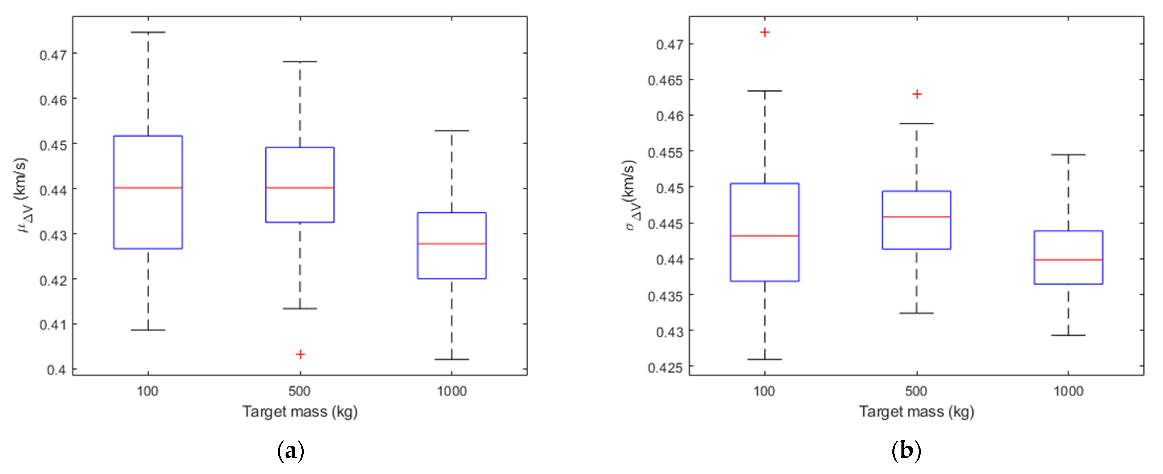
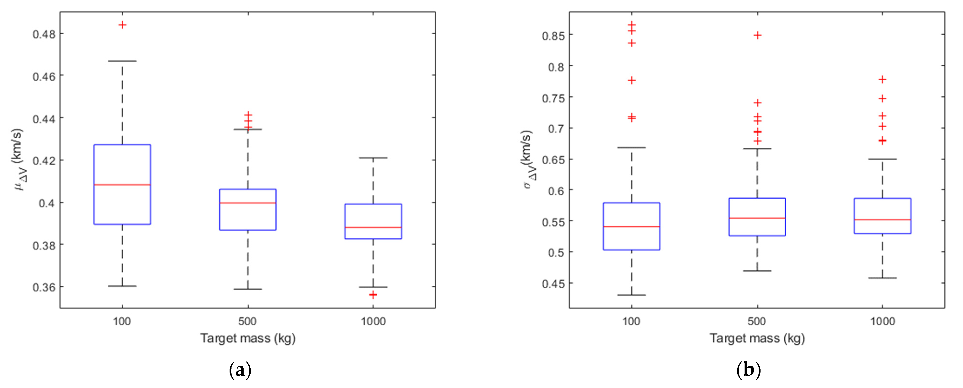
Figure 1,
Figure 2 and
Figure 3 show the boxplots of
μΔV and
σΔV in the different cases for the sample fragments. On each box, the central mark (i.e., the red line) indicates the median of the statistics parameter (i.e.,
μΔV and
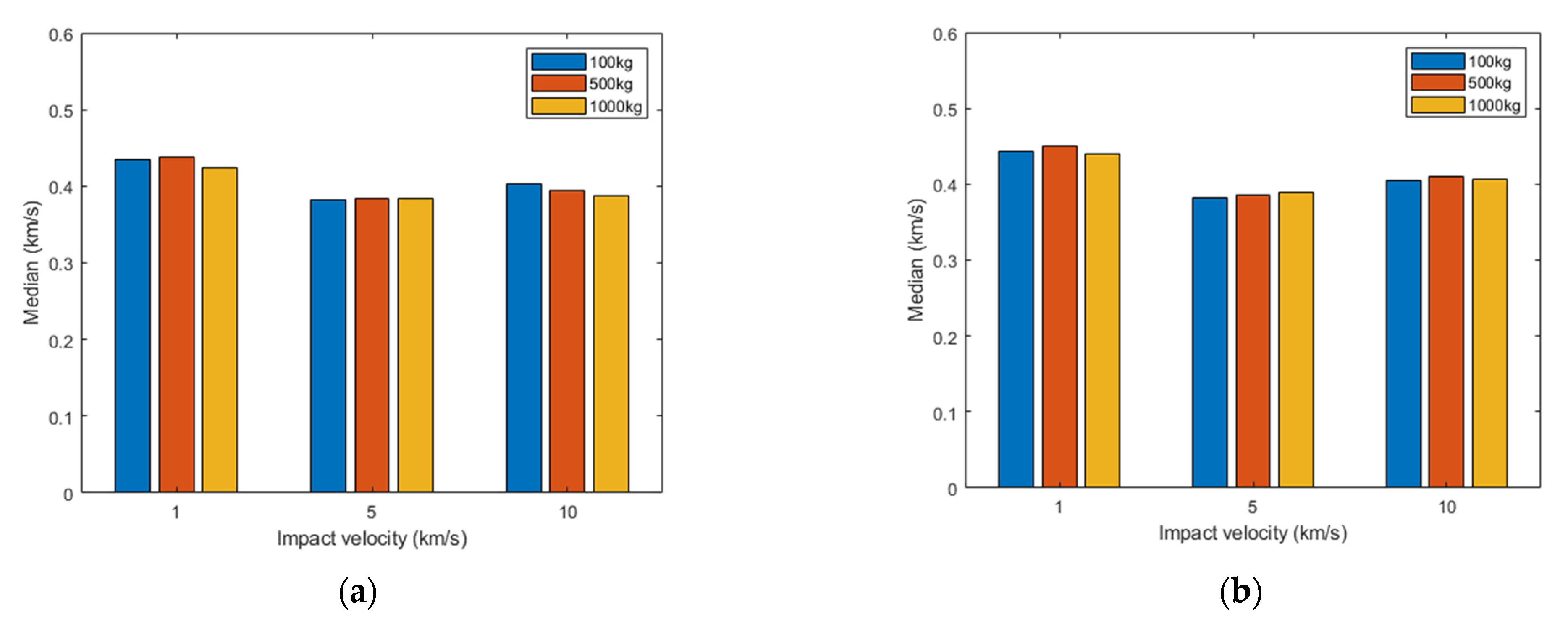
σΔV), the bottom and top edges of the box indicate the 25th and 75th percentiles, respectively. The difference between the 75th and 25th percentiles (i.e., the height of the box) is called interquartile range (IQR). The whiskers extend to a value equal to 1.5*IQR above the 75th percentile and 1.5*IQR below the 25th percentile. Outliers are the values beyond the whiskers and are plotted individually using the ‘+’ symbol. By looking at the mean and standard deviation distributions, for a fixed impact velocity, the Δ
V distributions are statistically similar regardless of the target mass. In fact, applying a two-sample t-test to the Δ
V distributions obtained with the same impact velocity and different target mass, the null hypothesis (i.e., the sample data are from populations whose expected means are the same) is accepted with 95% of confidence in all the cases. Moreover, the percentage variation of the median of the
μΔV and
σΔV distributions was computed for target mass equal to 500 kg and 1000 kg with respect to the case in which the target mass is equal to 100 kg. The results of this analysis are reported in
Table 1 considering different values of the impact velocity. The percentage variation is less than 5% for the median of
μΔV and less than 10% for the median of
σΔV.
To further support the above statement,
Figure 4 plots the median of the means of Δ
V distributions against the impact velocity for the different values of the target mass. There is not a clear trend between the median of the mean of Δ
V and the parent’s mass. This analysis shows that, for a known impact velocity, the velocity distribution of the fragments is not significantly affected by the parent masses, and thus, cannot be used to estimate the fragmented mass.
Therefore, as in previous works [
4,
28] the parameters estimation is based on the number of catalogued objects. This approach, however, presents three main challenges. Firstly, the limitations of ground sensors introduce an observability gap. In fact, depending on the altitude, only fragments greater than a certain threshold,
Lmin, can be detected and tracked (e.g.,
Lmin of order of 10 cm size at LEO and 1 m at GEO). Secondly, after a short time from the fragmentation event (FEV), the cloud of debris is not dispersed enough, and it is hard to correctly catalogue the different fragments of the cloud. Thirdly, especially for high energy collisions or for breakup events at lower orbits, a significant number of fragments decay due to the atmospheric drag. Thus, the epoch at which the fragments TLEs are known is important.
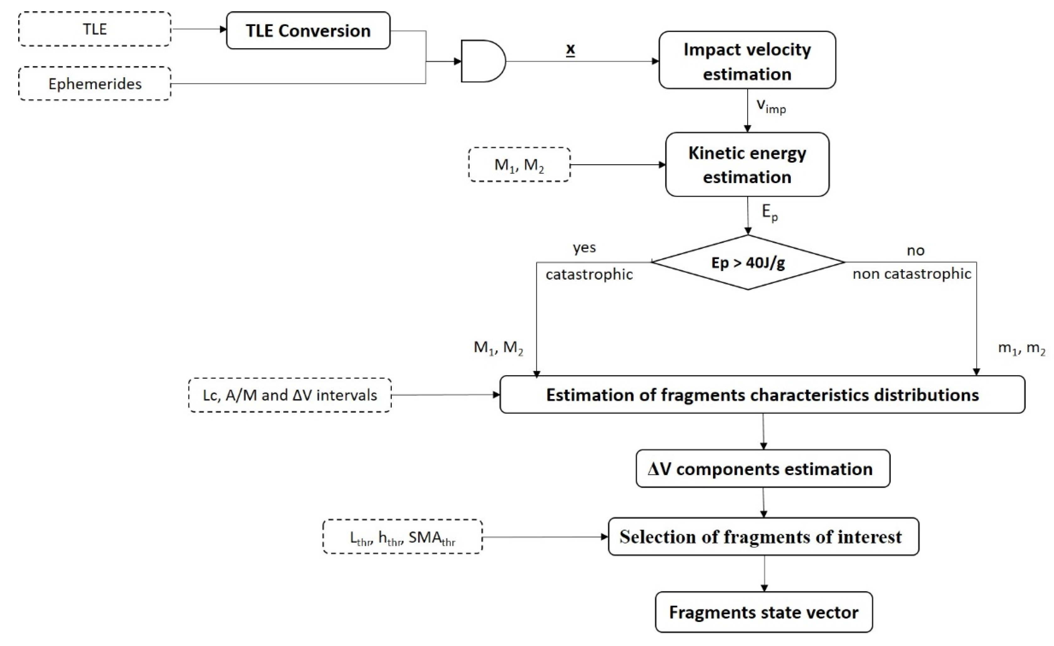
To better understand how to tune the model and to support the criteria adopted to filter the fragments generated by the SBM, a brief description of how the breakup model is implemented is provided. A scheme of the overall architecture is reported in
Figure 5.
The developed model takes as inputs:
The type of input file to load (i.e., ephemerides or TLEs). In both cases, the software extracts the state vector of the parent(s), x, either directly, in the case of ephemerides, or converting the orbital parameters to position and velocity, in case of TLEs. Moreover, the impact velocity is computed as the norm of the relative velocity difference between the two colliding objects.
Mass and size of the parents
After the kinetic energy estimation and the classification of the type of collision, the distributions of the fragments’ characteristics are estimated, as described in the previous section. Such distributions can be limited within user-defined intervals based on literature [
12]. In particular, at each step of the area/mass extraction (and hence of each fragment mass assignment), a check on the mass conservation principle is carried out. Specifically, fragments are extracted according to the normal procedure as described in
Section 2 until the difference between the sum of their masses (
Mtot) and the mass of the parent is lower than a tolerance threshold (i.e., 5%). If the extraction procedure leads to a value of
Mtot greater than the mass of the parent by more than 5%, the fragments with minimum
A/M probability in the current
Lc bin are removed. Then the Δ
V distribution is estimated. The SBM only provides the distribution of the Δ
V module for the fragments generated by the breakup event. To analyze the fragments’ evolution, a direction must be assigned to each Δ
V. This task must be done assuring that the conservation of momentum is met. Hence, an icosahedral grid was created whose nodes correspond to directions in a three-dimensional space [
26]. It is assumed that each node has the same probability to be associated to each fragment. The Δ
V, multiplied by the direction cosines corresponding to each direction, gives the velocity components of each fragment. Each fragment is therefore characterized by length, mass, area, and area/mass ratio, position at the fragmentation event (FEV), coinciding with the position of the parents, speed at FEV, computed as the sum between the speed of the parent and the Δ
V. The obtained set of fragments is then filtered by removing objects characterized by:
length smaller than a threshold value (Lthr) defined by the user,
negative semimajor axis (SMAthr), corresponding to a hyperbolic orbit, not of interest for the analyses of this paper. In fact, the possibility to track these fragments vanishes in time and their number is usually lower than 2% of the fragments over the size threshold.
altitude at perigee lower than 120 km (hthr), corresponding to a fragment that will re-enter before being catalogued.
The previous filtering is applied after assuring the conservation of momentum is achieved.
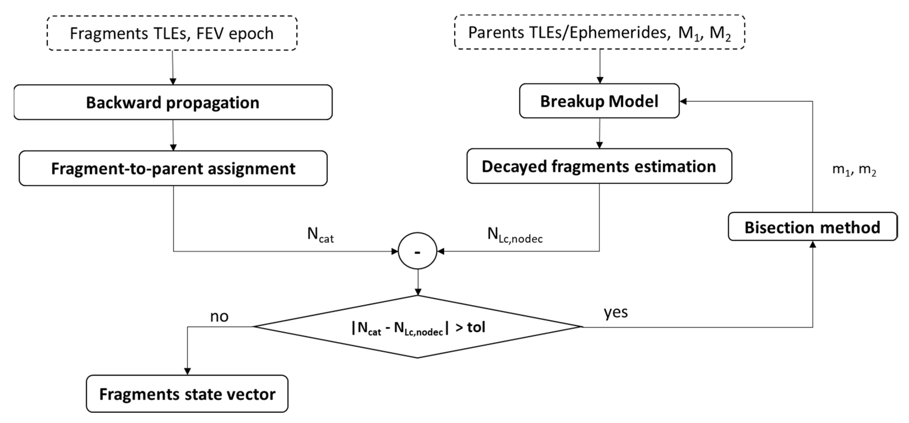
The Iterative Approach
An iterative logic based on the TLEs of catalogued fragments relevant to a fragmentation event is adopted to determine the input parameters of the breakup model and obtain the same number of real fragments within a certain tolerance. For the scope of this work, it is assumed that at the altitude of interest, all the fragments greater than a predefined threshold were catalogued. The logic consists of five main steps (as illustrated in
Figure 6):
The TLEs of the fragments are loaded and the orbital parameters are extracted. Let Ncat be the number of catalogued fragments.
A set of simulated fragments is generated from the breakup model using as default values the mass of the parents and their relative velocity. Let NSBM,Lc be the number of simulated fragments with a length greater than the predefined size threshold.
The catalogued fragments are backward propagated until the FEV. This helps to distinguish the two clusters of fragments belonging respectively to the target and the projectile out of a TLE file containing mixed fragments generated by the parents. The general principle is to compute the norm of the relative velocity between fragments and parents at FEV, and to assign each fragment to the parent corresponding to the minimum norm. In the case of orbital planes rotated by at least a few degrees with respect to each other, which will typically characterize collision geometries for very low eccentricity orbits, the concept has a direct analytical implementation based on inclinations and right ascension of the ascending node. In fact, it is well-known that a plane change requires a large value of the out-of-plane component of Δ
V. This is confirmed also from historic breakups, registering a maximum plane change of 3 degrees for the fragments with respect to their parent’s original orbit [
22]. Therefore, it can be assumed that, even with high energy collisions, the breakup fragments will only be dispersed a small amount from the parents’ orbital planes. Using the law of cosines for spherical triangles, the rotation of each fragment’s orbital plane with respect to target and projectile ones is computed:
where:
θtarg and
θproj are the angles between the fragment orbit plane and the orbit plane of target and projectile, respectively,
ifrag,
itarg, and
iproj are the inclination of the fragment, target and projectile orbit planes,
Ωfrag,
Ωtarg and
Ωproj are the right ascension of the ascending node of the fragment, target and projectile orbit planes. If
θtarg is smaller (larger) than
θproj, the fragment is assigned to the target (projectile).
This procedure allows splitting in two parts the iterative process and carrying out two separate analyses. Mass and cross section area of the fragments, necessary for the backward propagation, might be unknown, especially when a short time since the FEV passed. Therefore, a default value of A/M is assumed. However, the uncertainty on these values should not affect the out-of-plane dynamics and, hence, the assignment of the fragments to the two debris clouds.
- 4.
Estimation of decayed fragments: due to a negative ΔV or to the atmospheric drag, some fragments may decay in the time frame, ΔtFEV,TLE, between the FEV epoch and the last available TLE epoch. The number of decayed fragments, Ndec, can be negligible in the iterative process when many catalogued fragments, Ncat, are available. However, when Ncat is small, the number of decayed objects might represent a significant percentage, thus affecting the estimation of the fragmented mass. To consider this aspect in the iterative process, Ndec must be estimated. This is done by counting all the NSBM,Lc fragments having an altitude at perigee below 150 km. It is indeed reasonable to consider that the fragments with this characteristic decayed in the time frame ΔFEV,TLE.
- 5.
Iterative algorithm: the iterative algorithm operates until the following relationship is satisfied.
where
tol is a tolerance margin,
NLc,nodec is the number of not decayed fragments larger than the threshold (i.e.,
NSBM,Lc −
Ndec). The values for the tolerances depend on the statistical variability of EVOLVE over different runs, which increases as the fragmented mass (and consequently, the number of catalogued fragments) reduces. So, for
Ncat less than 50, a minimum tolerance of 0.3
Ncat is set. For
Ncat in the range 50–100 and
Ncat greater than or equal to 100, the tolerance values were scaled down (i.e., 0.2
Ncat and 0.1
Ncat, respectively).
Figure 6 shows a scheme of the iterative logic implemented.
When Equation (10) is not satisfied, the bisection method is applied to estimate the tuning parameters. As stated in the previous section, the tuning parameters are the fragmented masses of the two parents. The bisection method is applied to the number of target and projectile fragments separately.
The inputs to the algorithm are the number of catalogued fragments from the target and projectile clouds (
Ncat,targ and
Ncat,proj), the number of simulated fragments previously generated, with altitude of perigee greater than 150 km at FEV (
NLc,nodec) and the mass
MSBM,i, with
i = 1,2 (1 for the target and 2 for the projectile).
MSBM,i, is equal to the total parent mass (for catastrophic event) or the estimated fragmented mass by the SBM, according to Equations (2) and (3). If the number of simulated fragments is equal (within a certain percentage) to the number of real fragments, the algorithm is not executed, and the number of simulated fragments is the one generated by the SBM. Otherwise, the algorithm is executed. Let
Mi be the initial mass of the
i-th parent (i.e.,
i = 1 for the target and
i = 2 for the projectile);
mi,j be the estimated fragmented mass for the
i-th parent at the
j-th iteration;
mi,0 =
MSBM,i, be the initial mass the bisection method starts with; [
aj bj] be the interval in which the bisection method is applied. For
j = 1:
then, if
NLc,nodec > Ncat + tol:
both for catastrophic and non-catastrophic collision, while if
NLc,nodec <
Ncat − tol:
for catastrophic collision, and:
for non-catastrophic collision. For
j ≥ 2, both for catastrophic and non-catastrophic collisions:
where, if
NLc,nodec > Ncat + tol:
while, if
NLc,nodec < Ncat − tol:Equations (15)–(17) are valid both for catastrophic and non-catastrophic collisions. In all the previous cases, the bisection method is lower bounded by zero mass and upper bounded by the initial parent’s mass.
4. Results and Discussions
To demonstrate the effectiveness of the proposed iterative approach, two simulated and one real collision events are considered as test cases.
4.1. Simulated Collision Events
A collision is hypothesized assuming the masses of the parent objects, i.e., M1 and M2, the impact velocity and the corresponding fragmented masses (i.e., m1 and m2). By running the SBM using m1 and m2 as input masses, the reference values for the number of generated fragments, i.e., N1 and N2, can be obtained.
The goal of the proposed iterative approach is to estimate m1 and m2 assuming that all the observable fragments, i.e., those with characteristic length larger than 10 cm, are catalogued. To this aim, the iterative approach is applied using the total masses of the parents, i.e., M1 and M2, as initial guess. The SBM is then iterated until the convergence condition given by Equation (10) is met. At convergence, the number of generated fragments is indicated by N1,est and N2,est, respectively, while the corresponding fragmented masses is indicated by m1,est and m2,est, respectively.
The first test case is the simulation of a catastrophic collision. The orbital parameters of the simulated parents are listed in
Table 2.
With a, e, i, Ω, ω, ν being respectively the semimajor axis, eccentricity, inclination, right ascension of the ascending node, argument of perigee, and true anomaly.
The parent masses are M1 = 1000 kg, M2 = 800 kg and the impact velocity is equal to 14 km/s. It is assumed that only the following masses are involved in the fragment generation: m1 = 850 kg, m2 = 490 kg. With these values of masses, the SBM generates a set of N1 = 693 fragments from the target and N2 = 453 from the projectile.
The input data for the fragmented mass are set equal to the actual parent masses, i.e.,
M1 = 1000 kg,
M2 = 800 kg, while
vimp is set to 14 km/s. The application of the standard SBM would produce a number of fragments,
NSBM, about 14% and 58% more than
N1 and
N2, respectively. However, after 3 iterations, the proposed approach reduces this overestimate to 0.9% and 2.2%, respectively, while allowing the estimation of the fragmented masses with an error with respect to the assumed values of about 3% and 2%, respectively. Simulation results are summarized in
Table 3.
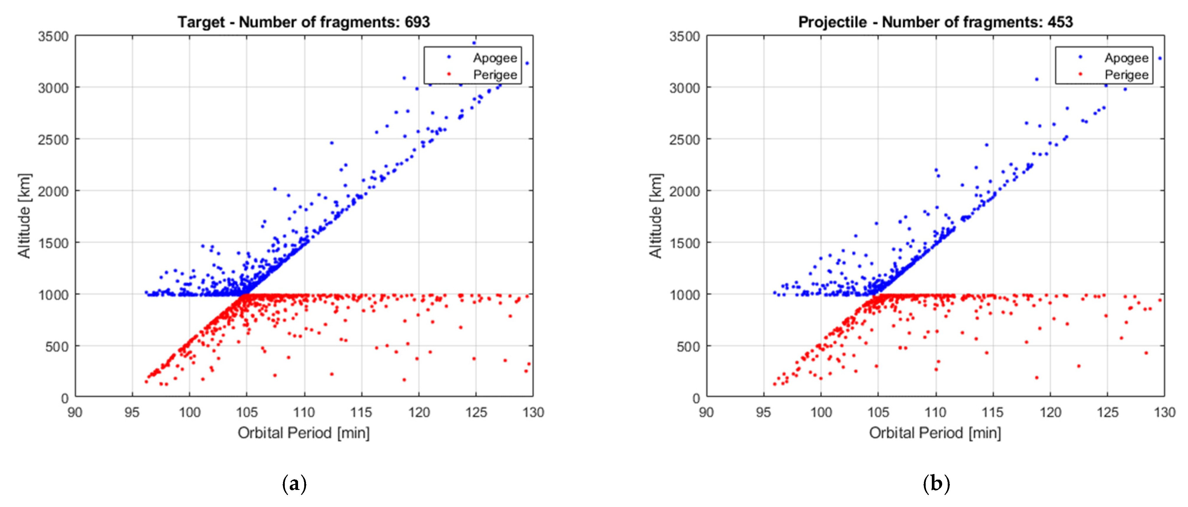
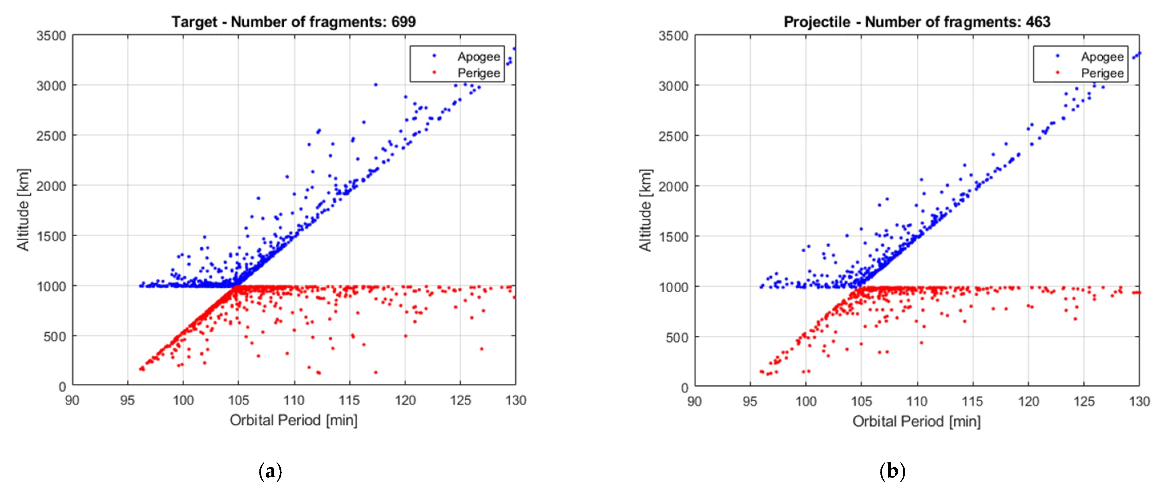
Figure 7 shows the distribution of the reference fragments in the
isin(
Ω)-
icos(
Ω) plane. In this plane, the distance of any point from the origin is equal to the inclination of the orbit plane of the fragment, while the ratio between the x-coordinate and the y-coordinate is equal to the tangent of the RAAN. The set of fragments derived from target and projectile gather in two regions have the same inclination of the parent objects, with a certain dispersion due to the collision. This is further supported by
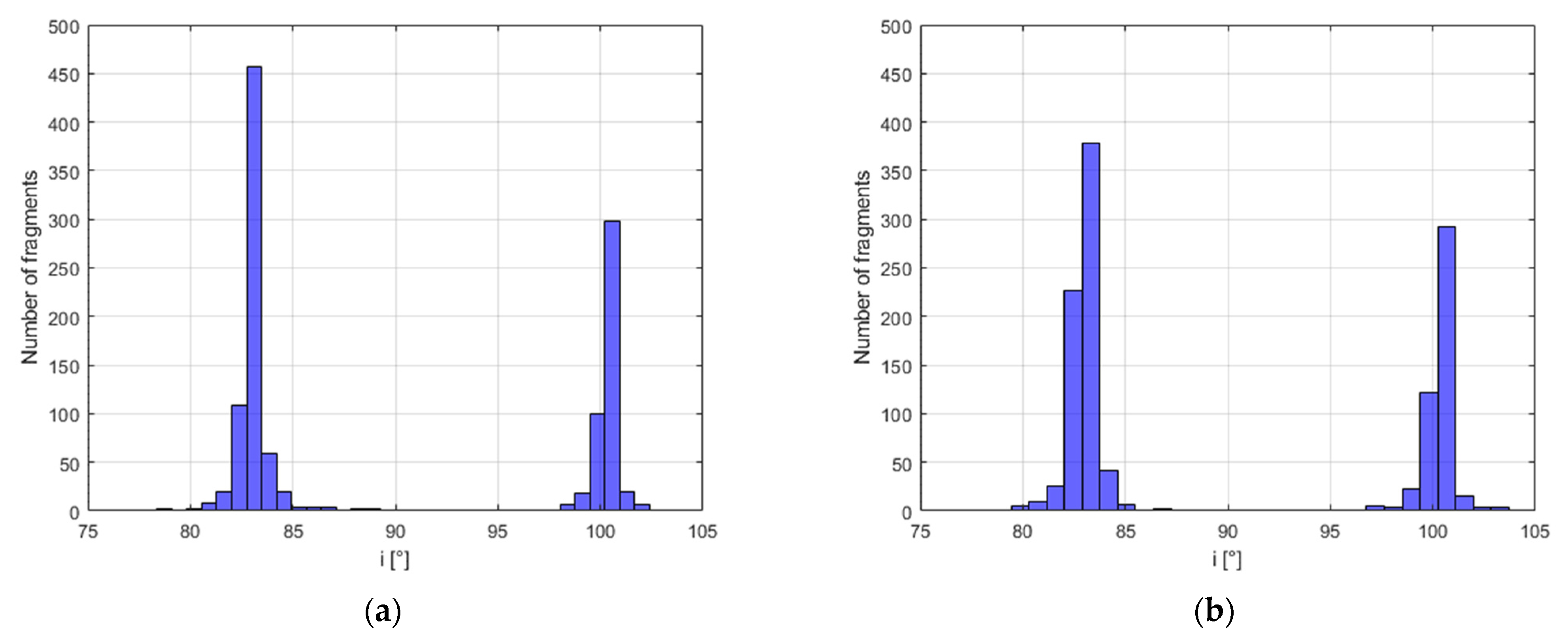
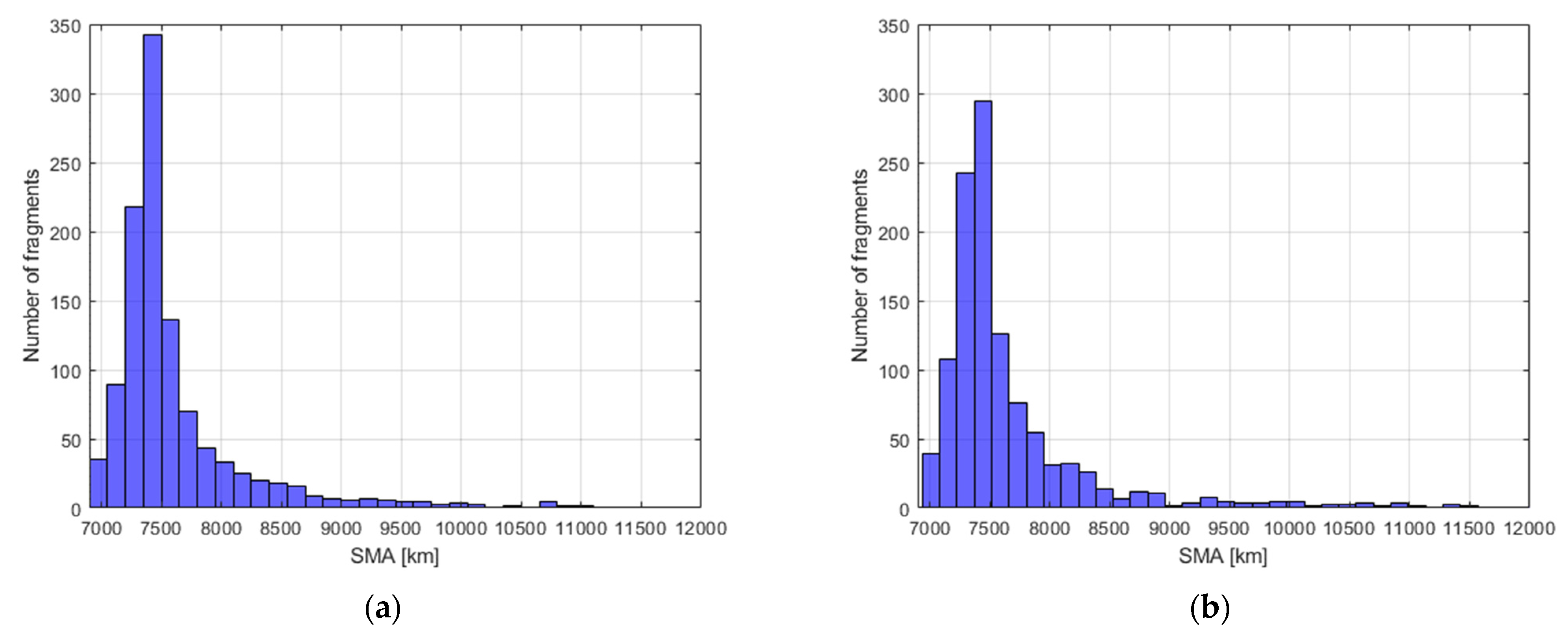
Figure 8, representing the histograms of the reference and estimated fragments in the range 75–105 degrees of inclination.
Figure 9 represents the histograms of the reference and estimated fragments in the range 6900–12,000 km of semi-major axis. This is representative of the Δ
V distribution and shows how they are qualitatively similar in the two cases. This is further supported by the Gabbard diagrams in
Figure 10 and
Figure 11.
As stated in
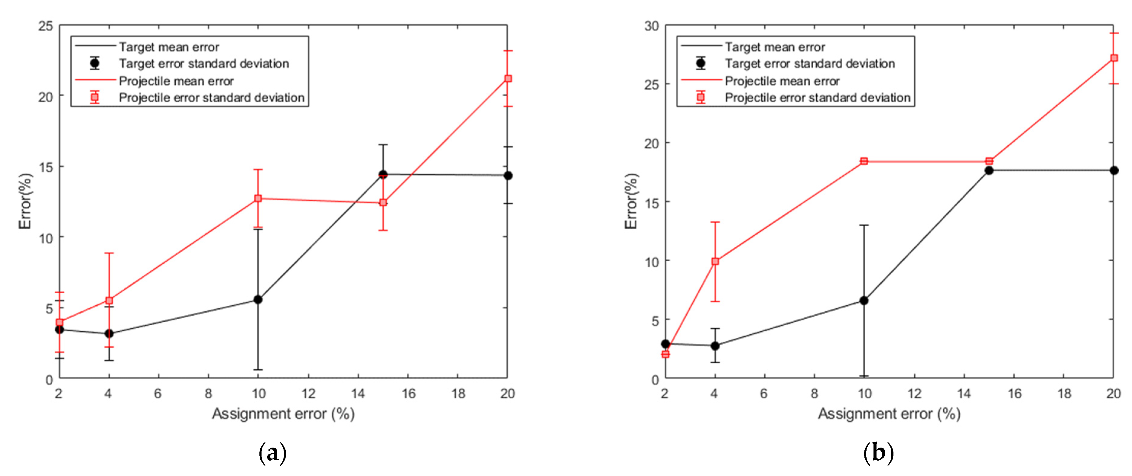
Section 1, a correct parent identification is not always guaranteed, and identification issues could lead to erroneously assigned objects. To consider this issue, an analysis of the method performance under this circumstance is carried out. It is assumed that a certain percentage of the projectile fragments was erroneously assigned to the target. In particular, the following percentages were considered: 2%, 4%, 10%, 15%, 20%.
Table 4 reports the number of fragments assigned to each parent considering the previous percentages. The obtained number of fragments is rounded up.
For each percentage assignment error, 100 runs were executed. For each run the mean
μnf and the standard deviation
σnf of the number of fragments greater than 10 cm, as well as the mean
μmf and the standard deviation
σmf of the estimated fragmented mass, were computed.
Figure 12a shows the percentage error associated to
μnf (solid line),
μnf − σnf and
μnf + σnf (error bars) for the target (in black) and the projectile (in red). Similarly,
Figure 12b shows the percentage error associated to
μmf (solid line),
μmf − σmf and
μmf + σmf (error bars) for the target (in black) and the projectile (in red). It must be pointed out that, for assignment errors lower than 10%, the output error is not necessarily due to the erroneous number of catalogued fragments, but also depends on the statistical variability of EVOLVE.
The second test case regards a non-catastrophic collision. The orbital parameters of the simulated parents are listed in
Table 5.
The parent masses are
M1 = 1000 kg,
M2 = 50 kg, and the impact velocity is equal to 1 km/s. It is assumed that only the following masses are involved in the collision:
m1 = 30 kg,
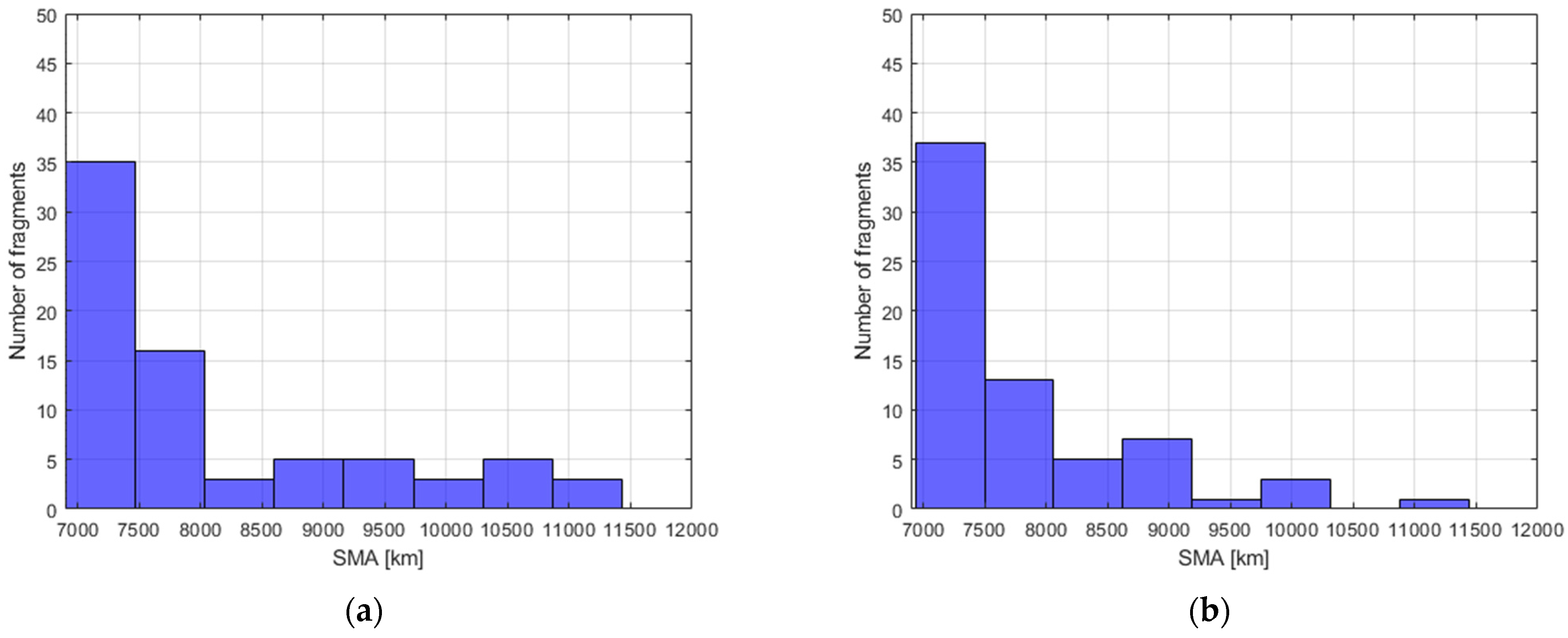
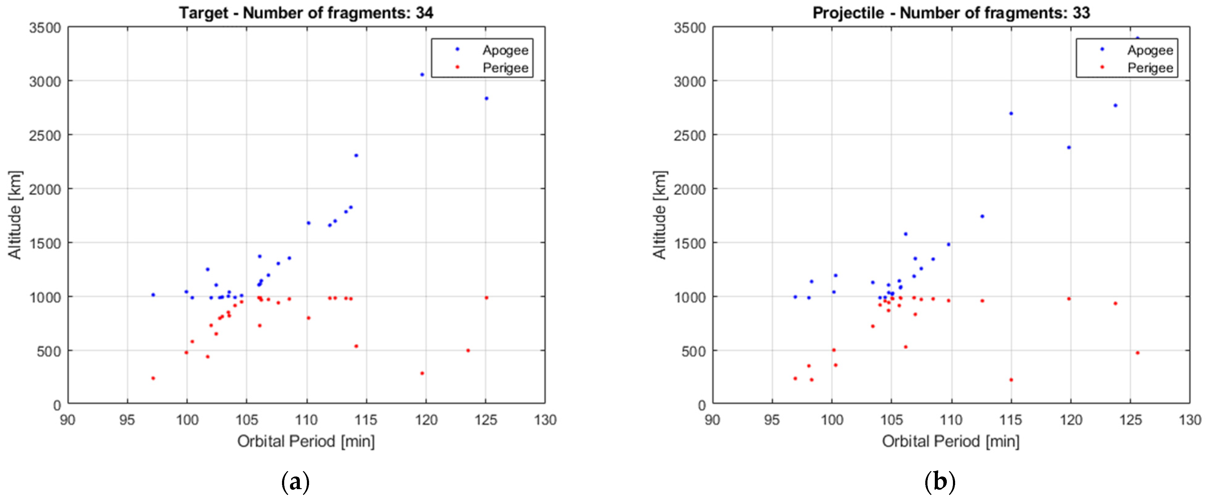
m2 = 30 kg. With these values of masses, the SBM generates a set of
N1 = 37 fragments from the target and
N2 = 38 from the projectile (as illustrated in
Table 6), considered as reference values. The input data are then set equal to the actual parent masses, i.e.,
M1 = 1000 kg,
M2 = 50 kg while
vimp is still equal to 1 km/s. Without the iterative approach, the SBM estimates fragmented masses,
MSBM, of 50 kg for both the target and the projectile (about 67% more than the assumed involved mass), while the number of generated fragments is equal to 68 and 74. Instead, the iterative approach allows reducing the fragmented mass estimation error down to about 17% of the assumed values. With regards to the number of fragments the SBM commits an error of 84% for the target and 94% for the projectile, while these values are reduced to about 8% and 13% by applying the iterative approach. These results are in accordance with Pardini and Anselmo [
27] that highlight how the outputs of the non-catastrophic collisions are worse than catastrophic collisions in the estimation of the number of fragments. The output of the second test case is summarized in
Table 6.
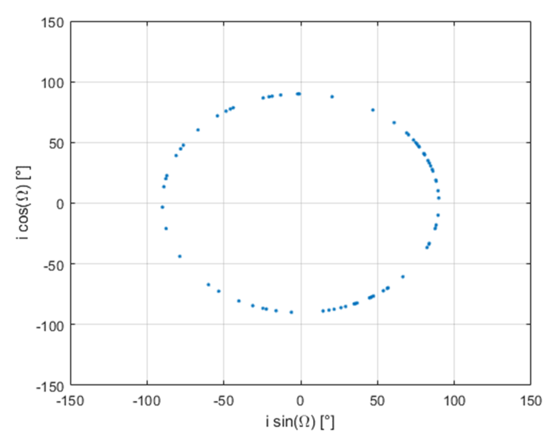
Figure 13 shows the distribution of the reference fragments in the
isin(
Ω)-
icos(
Ω) plane. Differently from the first test case, the set of fragments derived from target and projectile lie on the same circle corresponding to an inclination of 90 degrees. This is further supported by
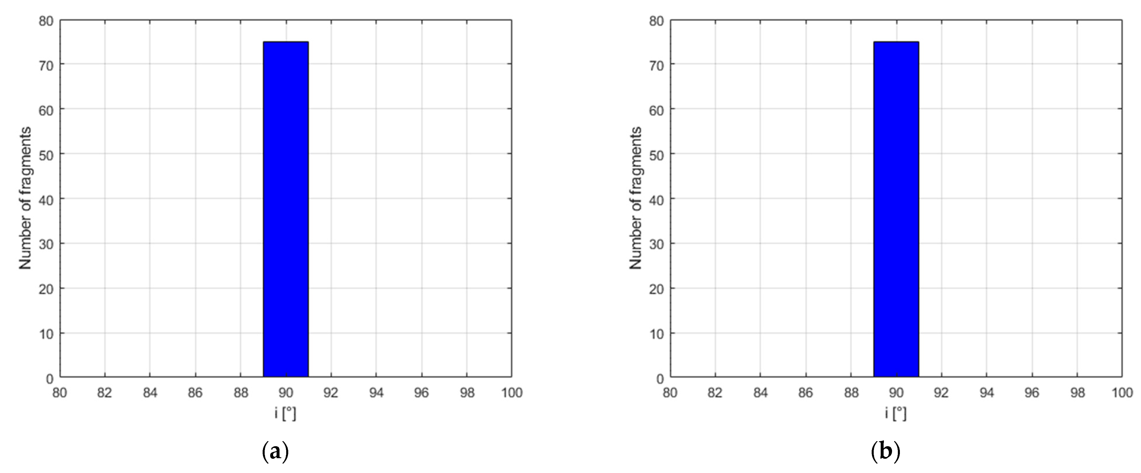
Figure 14, representing the histograms of the reference and estimated fragments in the range [80, 100] degrees of inclination.
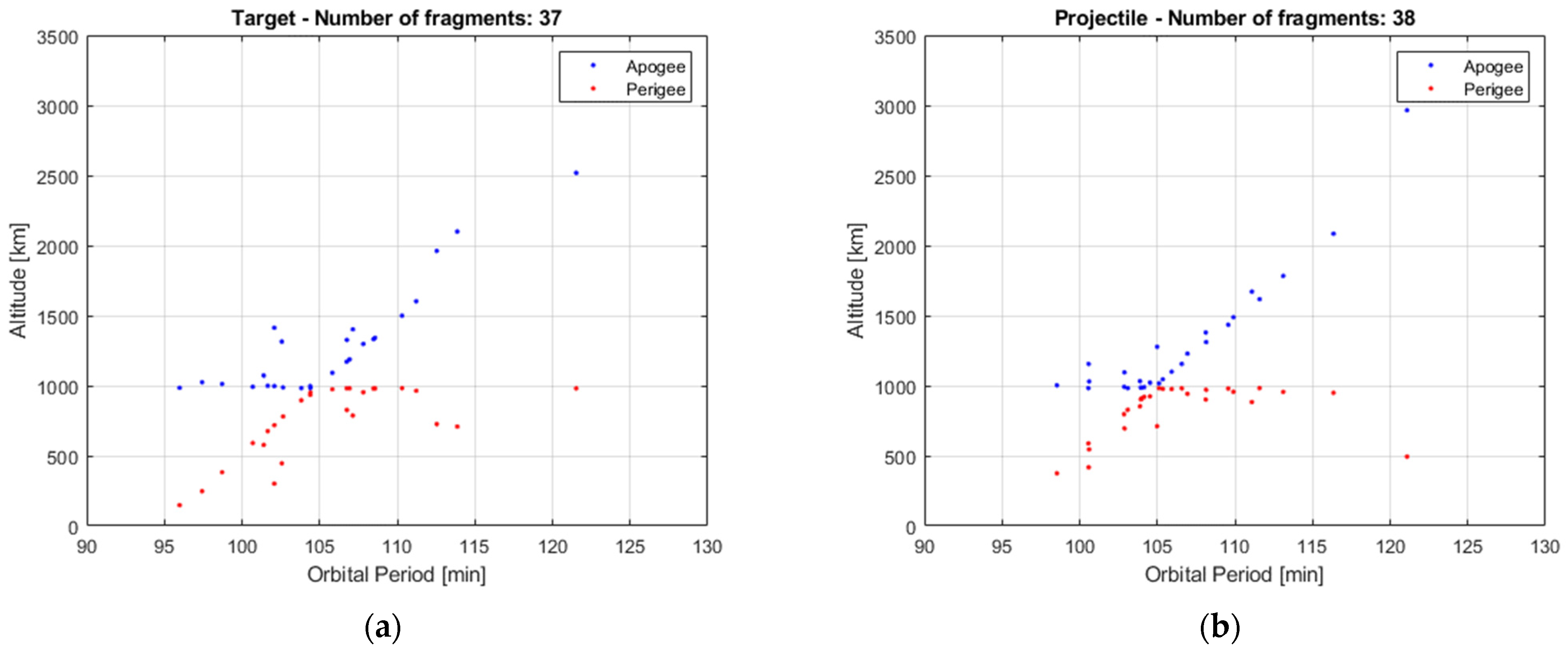
Figure 15 represents the histograms of the reference and estimated fragments in the range [6900, 12,000] km of semimajor axis. This is representative of the Δ
V distribution and show how they are qualitatively similar in the two cases. The Gabbard diagrams in
Figure 16 and
Figure 17 further support this statement.
4.2. Real Collision Event
The third test case is a real fragmentation event, namely the on-orbit collision between DMSP 5B F5 Thor Burner 2A (i.e., target) and the Catalogued debris 26,207 (i.e., projectile) happened on 17 January 2005 [
27]. Thor Burner 2A had a mass of 50 kg while the debris had a mass of 2.1 kg. The two objects collided at an altitude of 885 km with an impact velocity of 5.7 km/s. According to the SBM, since the energy-to-mass ratio is 62 J/g, the event is catastrophic and the number of fragments over 10 cm would be equal to 64 for the target and 0 for the projectile. However, only 6 fragments were catalogued [
27]. Hence, the SBM overestimates the number of target fragments by 967%. Assuming that all the catalogued fragments are associated to the target, the iterative approach, instead, estimates a fragmented mass of 18.75 kg for the target and 2.1 kg (i.e., the total mass) for the projectile. The number of fragments generated are
N1,frag = 6 and
N2,frag = 0 in accordance with the catalogue.
Table 7 summarizes all the data.
In all the previous test cases, the iterative approach provided reasonable tuning parameters to have a number of estimated fragments within a certain predefined interval. It is important to highlight that, even if theoretically possible, it is not useful to further reduce the percentage error. Indeed, due to the statistical nature of the SBM and the random extraction of the fragments’ characteristics, the output could have a variance greater than the pre-defined percentage error.
Some further considerations can be made with respect to the number of fragments. When the number of catalogued fragments is relatively large (e.g., more than 50 fragments), after breakup model tuning it is possible to extract from the simulated distributions sets of fragments which are consistent with the observed ones. When the number of catalogued fragments is very small, two major concerns arise. On the one hand, the type of fragmentation event (i.e., collision or explosion) may be itself uncertain. On the other hand, while it is possible to verify the consistency of observed data with theoretical distributions, the phenomenon cannot be replicated in simulations by random extractions.
4.3. Computational Cost Analysis
In general, the computational cost characterizing the proposed method is mostly related to the run of the SBM and so to the number of iterations required to reach convergence.
For the sake of analyzing the effect of the tolerance on the number of iterations, an additional simulated test case is considered. Two parents with mass equal to 800 kg collide with an impact velocity of 10 km/s. The collision is theoretically catastrophic. The algorithm is executed considering three different subcases:
Ncat greater than 100 (i.e., 500), between 50 and 100 (i.e., 60), and below 50 (i.e., 20) for both the parents.
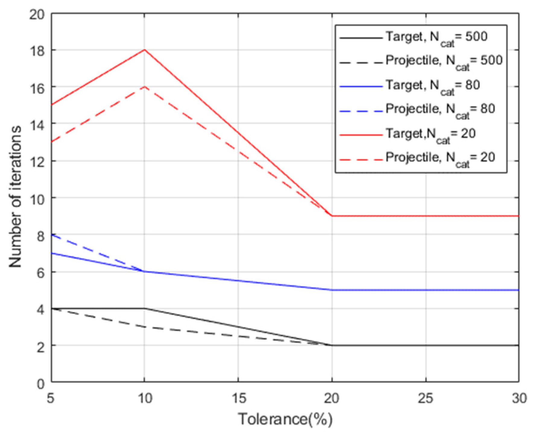
Figure 18 shows the number of iterations required, for the target (solid line) and the projectile (dashed line), to reach the convergence versus a tolerance value on
Ncat equal to 5%, 10%, 20% and 30%. In all cases, a relatively small number of iterations is required to reach convergence.


 ,
, 


