1. Introduction
The electrical flight control system (EFCS) is the industrial standard for commercial aircraft and has been widely used in the aviation sector, because it can improve the safety and performance of aircraft [
1]. Following the development of commercial aircraft, EFCSs are becoming more complex than before and the performance requirements (such as safety, reliability, maintainability, etc.) have increased [
2]. In response to this, fault-tolerant control (FTC) has gained importance because it can deal with system faults automatically, make the system stable, and regain the performance of faulty aircraft. Furthermore, fault signal monitoring has improved so that the integration of estimation and reconfiguration has attracted particular interest during the last decade [
3].
FTC consists of passive fault-tolerant control (PFTC) and active fault-tolerant control (AFTC) [
4]. In PFTC, a class of presumed faults are tackled by the designed controller, so that it is a special kind of robust control. The structure of the controller is simple because there is no need to add a diagnostic module, but the fault-tolerant capability is limited [
5,
6]. Thus, recently the focus has been on AFTC because of its outstanding fault handling capability [
7,
8,
9,
10,
11,
12,
13]. The main feature of AFTC is that it contains both estimation and reconfiguration. In most of the literature works, these two modules are designed independently in the FTC system, and the estimation is only used for monitoring or diagnosis. Moreover, the capability of it is often overrated, and very few articles concentrate on the integrated scheme of fault-tolerant controller design.
To design an active fault-tolerant controller capable of addressing the mentioned difficulties, it is necessary to develop an integrated design method, with no need for a prior knowledge of faults. There are few papers about the integration of estimator and controller. In [
14], a robust observer was presented to obtain system states and actuator faults. The linear matrix inequality (LMI) technique was utilized to reconfigure the controller. A disturbance observer was proposed to obtain fault signals in [
15]. Based on the designed estimator, a controller is reconfigured using a modified fuzzy dynamic output feedback method to address faults (actuator or sensor) and mismatched input disturbances. The authors of [
16] presented an integrated strategy of AFTC where the PD extended state observer was designed to estimate system states and actuator/sensor faults, and the control law was designed using a modified LMI-based
robustness procedure. A reduced-order observer was to deal with the problem of fault estimation and a reconfigurable controller was built for nonlinear discrete-time systems in [
17]. In the existing integrated strategy, adaptive control and robust control were used, and the theorems are mathematically correct. However, there are several weaknesses when applying this in EFCSs, because of the many assumptions about the rank of the system matrices.
Furthermore, the phenomenon of actuator saturation is important in the integrated reconfigurable strategy, because aircraft actuators are physically limited and faults will decrease their capability. Many works have focused on the combination of anti-windup and FTC [
18,
19,
20,
21,
22,
23,
24]. The common design process is designing an original reconfigurable controller and modifying it using different anti-windup methods. In the cited literature, the magnitude saturation has been well addressed, however the rate limiting (another important constraint) has been ignored. Moreover, the integrated design strategies which can tackle the pairing between the estimation and reconfiguration have not been used, so that the real-time reconfigurable performance can not be guaranteed.
With respect to the mentioned problems, the contributions of this paper mainly include the following two points. First, different from the works in [
7,
8,
9,
10,
11,
12,
13], an integrated reconfigurable control strategy is presented to cancel the pairing between estimator and controller, and to improve the performance of the controller. Moreover, compared with the works in [
14,
15,
16,
17], both actuator and sensor faults are considered in the design of integrated fault-tolerant control. Second, two common actuator constraints (magnitude and rate) are considered to design the anti-windup FTC scheme using different techniques. In contrast with the proposed anti-windup reconfigurable controller, most of the existing anti-windup schemes can just address the magnitude saturation [
18,
19,
20,
21,
22,
23,
24].
The rest of this paper is organized as follows.
Section 2 gives the normal/post-fault aircraft modeling. In
Section 3, the integrated strategy and their anti-windup modifications are given. In
Section 4, the simulation results and analyses are presented, and
Section 5 reports conclusions of this paper.
The following notations will be used throughout the paper: I signifies an identity matrix, signifies the diagonal matrix, and signifies the pseudo-inverse.
2. System Modeling
It is necessary to construct an appropriate aircraft model for the integrated design. The model of an aircraft during normal operation (without faults and actuator constraints) is described as
where
denotes the system state, in which
is the forward velocity,
is the vertical velocity,
q is the pitch angle rate,
is the pitch angle, and
denotes the system output, and
denotes the system input, in which
is the perturbation from trim in the
ith elevator.
A,
B, and
C are the system matrix, the input matrix, and the output matrix, respectively. The detailed expressions are shown in
Appendix A.
If the aircraft operates in the presence of actuator and sensor faults, system (
1) can be rewritten under the fictitious multiplicative fault formulation as
where
denotes the controller outputs,
denotes the fictitious multiplicative actuator fault value,
is an indication matrix,
is the effectiveness factor,
denotes the additive actuator fault value,
d denotes the external disturbance,
denotes the measured output, and
denotes the sensor fault value. The detailed modeling and analysis for faults can be found in reference [
25].
Assumption 1 ([
5]).
All of the faults and disturbance in (2) are norm-bounded, and the first time derivatives of faults are norm-bounded, too. Considering Assumption 1, we can augment the faulty system (
2) into
where
,
,
,
,
.
3. Integrated Strategy and Anti-Windup Modification
In the AFTC strategy, there is a pairing between the estimation and reconfiguration, that is, the controller needs fault information provided by the estimator, and the estimator needs to know which strategy is available for reconfiguration [
5]. Moreover, the actuator saturation is the most common nonlinearity in a control system and affects its stability [
26]. Thus, the integrated fault-tolerant control scheme and its anti-windup modification are important for EFCS because they guarantee the aircraft to track the command signal in the presence of actuator faults and saturations. Inspired by this problem, a novel integrated anti-windup method for linear systems is presented.
3.1. Integrated Reconfigurable Controller Design
An integrated scheme is utilized to design the reconfigurable controller in this subsection. In the augmented faulty model (
3), the unknown fault values
,
, and
are contained in
and are obtained by using the diagnostic module. The design procedure of the integrated strategy contains three steps: (1) Design a reconfigurable controller to control the aircraft to track the desired command, (2) design a fault estimator to estimate the states of the augment faulty system, and (3) calculate the undecided parameters of the controller and estimator by analyzing the stability of the overall system.
Augment the healthy system (
1) into
where
,
,
,
.
The reference control law is chosen as
where
is the controller state vector,
r is the command signal, and
and
are control gains.
Thus, the reference model (as a command generator) represented by the augmented system (
4) and the reference controller (
5) is obtained as
where
,
,
,
,
.
The system dynamics is completely controllable by calculating the controllability matrix, and the detailed data are given in the
Appendix A. An optimal control technique (such as LQR) is used here to adjust the reference controller gains. The detailed design procedure can be found in [
7], and thus it is omitted here.
Moreover, the system dynamics can be derived from (
3) by introducing a new control variable
as
where
,
,
,
,
,
.
Defining the error between the reference model state and the system state as
, a reconfigurable control law is chosen as
Substituting the reference model (
6), the system (
7), and the control law (
8) into the error expression yields
where
.
and are control gains, and are designed by analyzing the stability of the post-fault aircraft model, that is, ensuring where is a Hurwitz matrix. The term represents the errors between the faulty aircraft and the reference model, and it affects the control performance. Furthermore, the control gains are calculated by an adaptive integrated strategy to address the unknown external disturbance and system parameter errors.
In the design procedure of the fault estimator, an observer is described as
where
is the observer state vector and
is the estimate of
. The remaining undefined matrices are designed observer gain matrices.
The design objective is to make sure that the error
between the faulty system state
and its estimate
converges to zero. Substituting (
3) and (
10) into
yields
where
,
.
Remark 1. Based on the works in [27,28], the rank condition for the designed observer (10) is , where is the coefficient matrix of in (3). As is chosen as an identity matrix I in this paper, the rank condition is satisfied. The observer matrices are designed by analyzing the stability of the system, that is, ensuring
, where
M is Hurwitz. The term
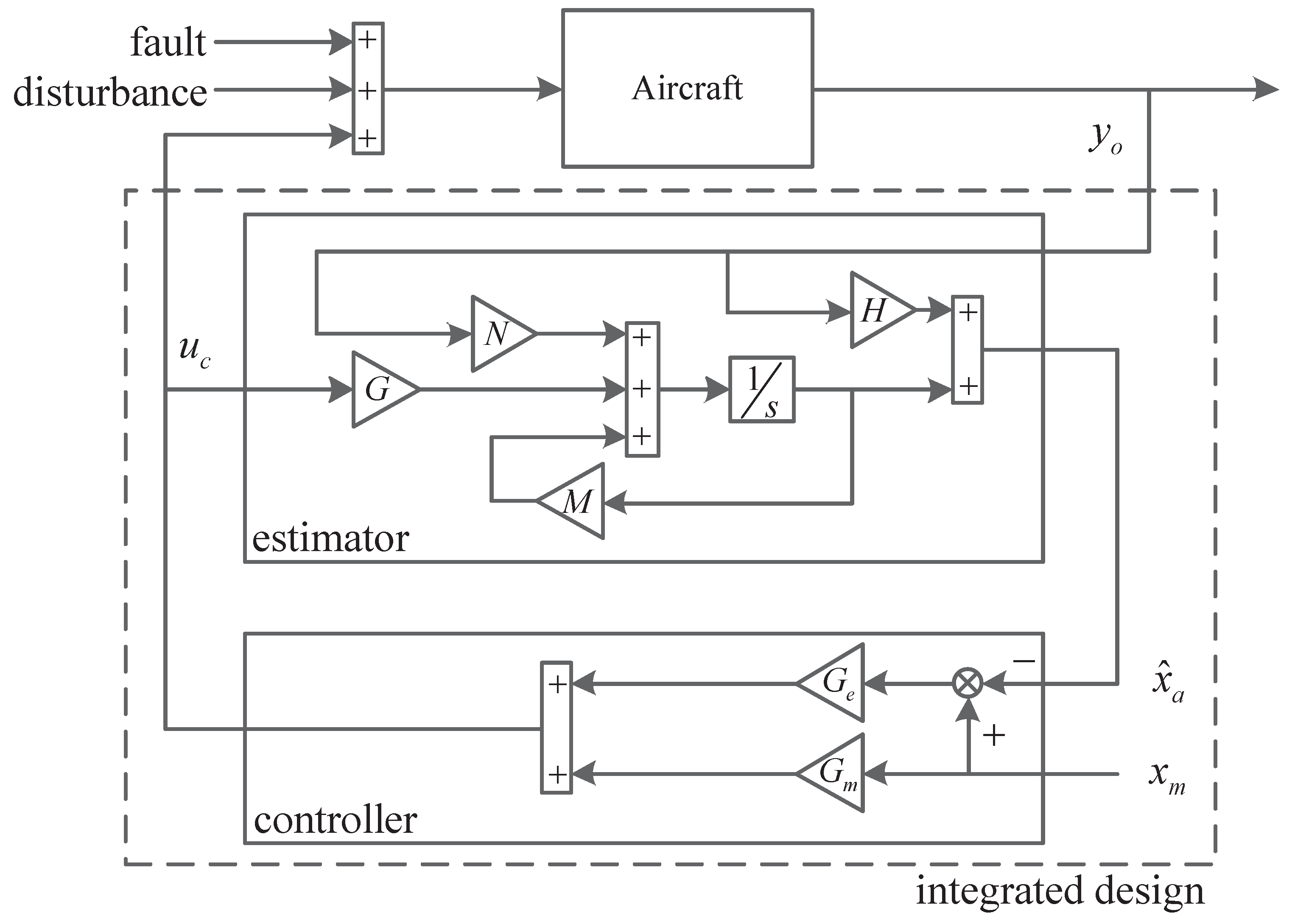
represents a coupling between estimator and controller, and it affects the estimation performance. The integrated scheme is shown in
Figure 1. The following theorem is proposed to guarantee the stability of the overall system and to calculate the corresponding adaptive adjustment laws.
Theorem 1. The integrated system consisting of (3), (8) and (10) is asymptotically stable if the gains of controller and estimator hold so thatwhere , , , and are symmetric positive-definite matrices. Proof. Rewrite the controller error dynamic system as
where
is a Hurwitz matrix,
, and
.
A Lyapunov candidate function is chosen as
where
,
.
Setting
and
so that
and
, the first and second items of (
12) are obtained. Moreover, setting
yields
. Thus, the rest of (
15) is transformed into
where
.
As
is Hurwitz, it can be concluded that
is the unique solution of the following Lyapunov matrix equation:
where
is any symmetric positive-definite matrix.
Considering (
14) and (
16),
and
hold. This completes the proof of Theorem 1. □
Remark 2. The errors and are always nonzero in the application so that it is necessary to integrate the estimator and the controller. The adaptive laws cancel the adverse effect of the coupling and improve the capability of the reconfigurable control.
3.2. Anti-Windup Mechanisms
Actuator constraints consist of rate and magnitude saturation. In this paper, a modified software rate limiter (
) is utilized to address the rate constraint problem. As shown in
Figure 2, the plants “
” and “
” consist of actual aircraft models, “
” represents the ultimate reference controller (the original controller with/without a compensator), “
” represents the ultimate reconfigurable controller, “
M” is the reference model, and the actuator “
A” is position-controlled and is subject to saturation of physical systems (i.e., they only provide a certain amount of force or moment). In this scheme, the reference controller is modified by
, and a signal
has taken the place of the limiter in its quasilinear part. The reconfigurable controller can also be modified by
, and another signal
has taken the place of the limiter in the post-fault model. If the physical limitations of the actuators are not considered in the design procedure, the control performance will not be satisfactory and could possibly even lead to disastrous consequences. It is difficult to design integrated anti-windup controllers because of the different controller structures. The type of
(the Laplace transform of
) and
(the Laplace transform of
) are denoted as
and
, respectively [
29].
Assumption 2 ([
30]).
Whether actuators work in saturation or not, the normal and post-fault aircraft with are stable, and two feasible conditions are and . Theorem 2. The stable system with rate limiters will exhibit asymptotic stability in response to the injected signals and , if the types of ultimate controllers are more than zero.
Proof. The block diagram algebra for the normal system can be got from
Figure 2 as
where
is the error,
R is the command signal, and
Y is the system output. The majuscules denote the Laplace transform of their corresponding time functions. The actuator “
A” is ignored in this algorithm, because the linear part of “
A” is insignificant and the rate constraint in it can be canceled by
. The detailed actuator model is shown in
Appendix A.
Applying the final value theorem, it can be obtained that
As , the type of the first item is and the type of the second item is . The stable normal system with rate limiters is going to achieve asymptotic stability if and , i.e., . Considering Assumption 2, should hold.
Furthermore, the block diagram algebra for the faulty model is shown as follows:
where
,
, and
denote the plant elements, respectively, and
is the ultimate expression of
. Other majuscules are the Laplace transforms of their corresponding signals.
Applying the final value theorem, it can be obtained from (
20) that
In a similar way, all the types of terms on the right-hand side of (
21) should be less than zero. Thus,
should hold. This completes the proof of Theorem 2. □
Remark 3. In this paper, satisfies , so that it is not necessary to add a compensator to the original controller; however, does not satisfy , so that in this case the ultimate controller can be defined with a compensator as .
Remark 4. Based on the work in [30], the software rate limiters can provide enough stability margins for the linear design. Assumption of closed-loop stability is just the first step to analyze Theorem 2, so that the final value theorem can be utilized. We can use the asymptotic stability to derive a condition about the type of the injected signals and the type of controllers. The designed rate limiters and compensators may decrease the performance of the unconstrained system, but the performance of the constrained system is improved. For the magnitude saturation problem, as the reference controller and reconfigurable controller have different block diagram architectures, different schemes should be used to modify these two controllers. An observer-based scheme is utilized to modify the reference controller to mitigate windup, as shown in
Figure 3. The control signal will not reflect the plant if there is a mismatch between
and
, which is the reason causing windup. The modified reference controller is given as
where
is the designed gain matrix. The design task is choosing
such that
is Hurwitz. An effective design procedure is to analyze the difference between a system with actuator constraint and a system without it. The unconstrained normal system with state vector
is shown as
and the constrained normal system with state vector
is shown as
Finally, the mismatch between the two systems is shown as
. Subtracting (
23) from (
24), the mismatch system is shown as
Assuming
can be decomposed as
and choosing
, the gain
is designed as
where
is the last
columns of
, and
is the remaining column of
. The closed-loop system exhibits asymptotic stability.
Remark 5. The observer-based approach is intuitively appealing as the concept of the observer is widely used [26]. Amplitude constraint is addressed by feeding back the error between and to the reference controller, and it will not be modified when . As shown in
Figure 4, the anti-windup problem in the reconfigurable controller is tackled by using a modified conditioning technique. “
O” represents the estimator, and “
” represents the reconfigurable controller consisting of a compensator and a software rate limiter.
is chosen as the reference signal and the controller is described as
In the conditioning technique, an auxiliary input
, which is called realizable reference, is chosen as a new reference signal to make sure that there is no difference between
and
. The new controller is
Note that the actual reference signal
does not appear in (
28), so that an assumption on the present realizability (
) of the control is held as
The
is calculated by subtracting (
29) from (
28) as
where
is the designed gain.
Remark 6. In the modified conditioning technique case, the realizable reference removes the effect of the nonlinearity on the system input, so that the reconfigurable controller is “conditioned” back to the unconstrained mode as soon as it can.
4. Application Example
The integrated anti-windup scheme is simulated on a numerical model of Boeing 747, which is trimmed at straight and level flight. The external disturbance is defined as a uniform “1-cosine” vertical gust [
31]. Two flight conditions are shown in
Table 1 and
Table 2, respectively. The detailed data for this aircraft are obtained solely from a Boeing 747 simulator description (Boeing D6-30643) and are provided in the NASA report [
32].
4.1. Anti-Windup FTC in Condition 1 at 0.5 Ma and 20,000 ft
In this condition, the reference command is a step signal given at 2 s, the elevator is locked in , the surface deflection loses effectiveness, the bias of the sensor is , and all faults are given at the same time (0 s), that is, , , , and . The limits of magnitude and rate are and /s, respectively.
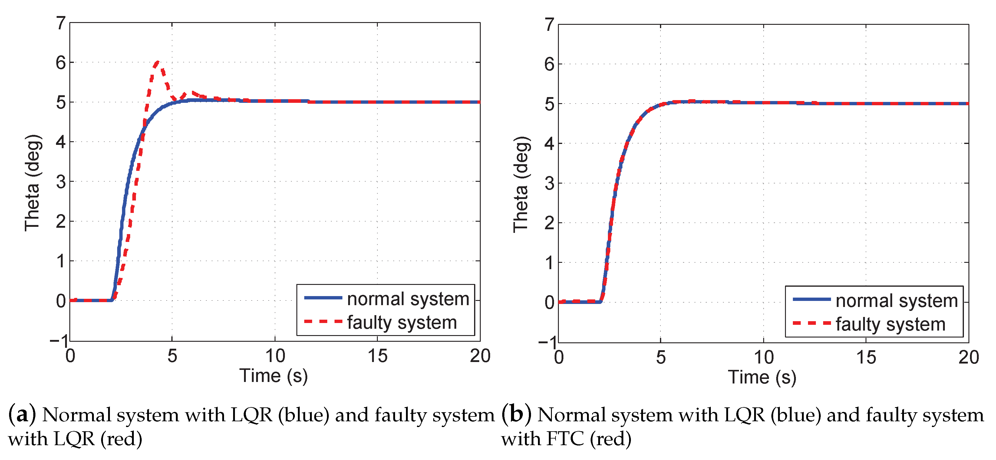
Figure 5a shows the necessity of the FTC strategy because there is a significant decrease for control performance in the post-fault aircraft with LQR (red) than in the healthy aircraft with LQR (blue). In
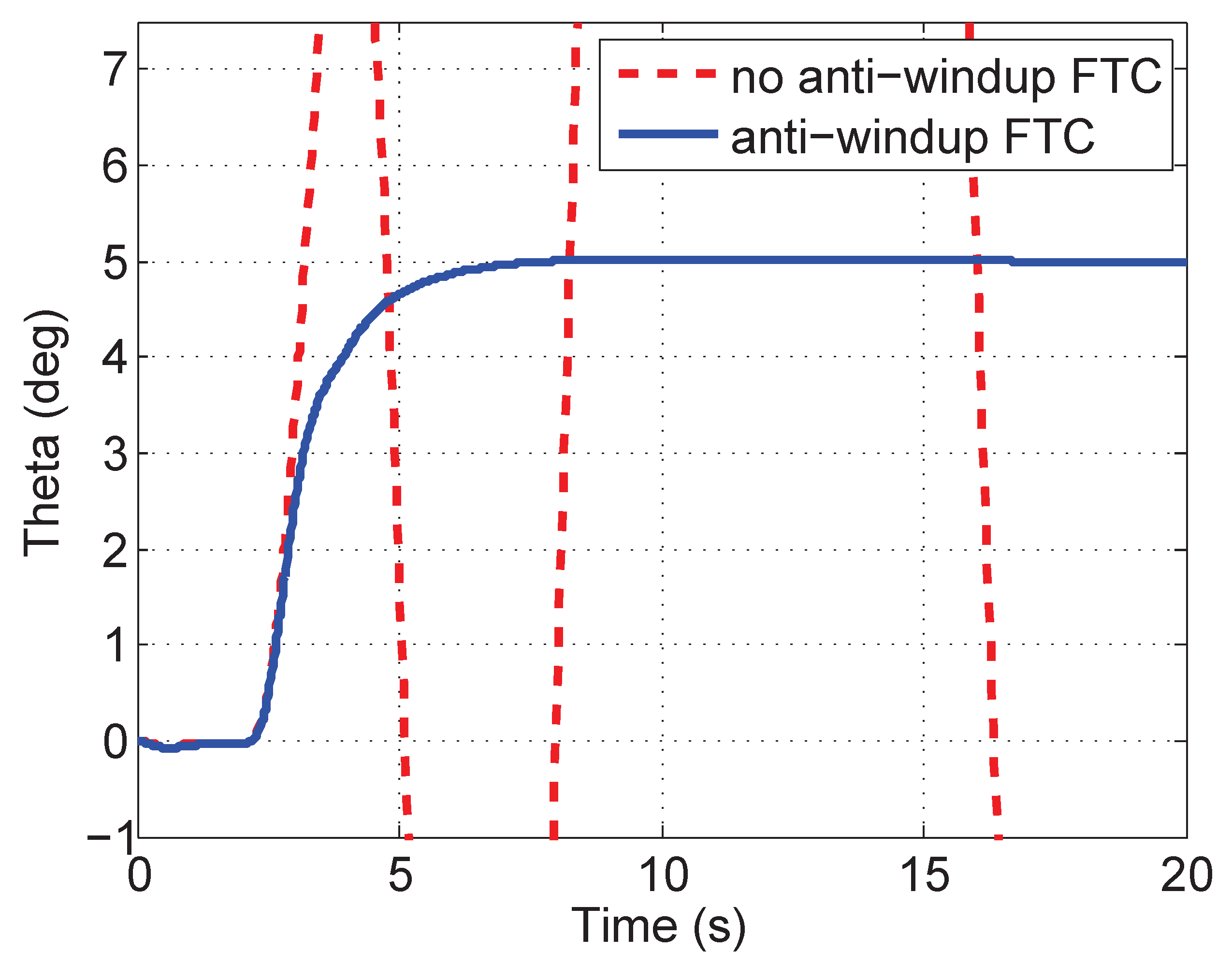
Figure 5b, however, the control performance of FTC in the post-fault aircraft (red) is nearly the same as the one of the LQR in the normal aircraft (blue). When there are magnitude and rate saturation modules in the actuators, as shown in
Figure 6, the FTC method without anti-windup (red) will reduce the control performance or even make the system unstable. The anti-windup reconfigurable method is designed using a compensator (blue) to deal with the windup phenomenon and regains the performance of the post-fault aircraft.
Figure 7 shows the estimates of actuator and sensor fault values. They are estimated accurately using the proposed estimator at about 5 s after occurrence. The faulty aircraft model with actuator saturation modules (magnitude and rate) is used in
Figure 8. It compares the actuator deflections (
,
,
,
) and rates (
,
,
,
) between the original FTC method and the FTC with capability of anti-windup. The actuators with FTC meet their constraints so that the aircraft is unstable; on the contrary, the proposed anti-windup modifications mitigate the effects of saturation and guarantee the stability of the aircraft.
4.2. Anti-Windup FTC in Condition 2 at 0.8 Ma and 40,000 ft
A higher altitude and faster condition than before is considered to verify the effectiveness of the presented method, where is a step signal given at 2 s, is locked in , loses effectiveness, and the bias of the sensor is . That is, , , , and . The limits of magnitude and rate are and /s, respectively.
Figure 9 shows the pitch angles of the normal and faulty aircraft. From
Figure 9a, it can be seen that the reduction of the control performance for the faulty aircraft with LQR (red) is more serious than the one in
Figure 5a. However, FTC in the faulty system in
Figure 9b (red) can also recover the control performance of the healthy system with LQR (blue). In
Figure 10, we can get the same results as in
Figure 6.
Figure 11 shows the estimates of fault values.
Figure 12 shows the actuator outputs of FTC and anti-windup FTC in the faulty aircraft with two kinds of saturation modules. As actuator 1 is locked in
, actuators 2 and 3 meet their constraints so that FTC cannot guarantee the post-fault aircraft stability. On the contrary, the anti-windup FTC can cancel out the nonlinear windup phenomenon in the actuators and make the faulty aircraft stable.


