1. Introduction
Modern compressors and fans have tip sections of the blades typically operating at supersonic relative inlet velocity and subsonic outlet velocity; ultimately, this leads to fewer compressor stages and lighter, more compact propulsors. At supersonic inlet conditions, the flow field is characterized by a complex shock wave system, whose strength and interaction with the boundary layer largely affects pressure rise and entropy generation. Moreover, these phenomena strongly deteriorate the performance at off-design conditions and reduce surge and rotating stall margins [
1]. For these reasons, the design of supersonic blades is critical, and new shapes are designed ad hoc for given operative conditions, rather than chosen from a family of profiles. Nowadays, three-dimensional aerodynamic models, in which the entire blade is simulated, are widely used; nevertheless, two-dimensional analysis is still fundamental in blade design and can provide extremely accurate results, more difficultly matched by more complex simulations. Computational Fluid Dynamics (CFD) in conjunction with automatic methods has been widely used in numerical simulations and optimization of supersonic blades. In [
2], a multi-objective optimization of a 2D S-shaped supersonic profile, operating at a unique incidence condition, was conducted using a Kriging-assisted evolutionary algorithm in order to minimize total pressure losses and to maximize the pressure ratio. In [
3,
4], one-dimensional analytical shock-loss models were developed to predict overall total pressure losses. Upon these models, optimizations were conducted to reduce losses on two baseline geometries, acting on profile shape and thickness distribution. In [
5], an optimization based on differential evolution was carried out to reduce losses in a supersonic blade, parametrizing the camberline only. A numerical investigation on potential improvement of the transonic compressor by using tandem rotor blades was carried out in [
6]. In [
7], a 3D optimization of tandem rotors, National Air and Space Administration (NASA) Stage 35 was carried out using the Non-dominated Sorting Genetic Algorithm (NSGA II) and the backpropagation Artificial Neural Network (ANN) technique to maximize the total pressure ratio and reduce the total pressure loss coefficient. Typical improvements achieved in various optimizations were around 20% for efficiency and 3% regarding the pressure ratio. This paper presents a multi-objective multi-point aerodynamic optimization of a two-dimensional supersonic cascade that minimizes the total pressure-loss coefficient and maximizes the pressure ratio. The computational two-dimensional model was validated upon experimental data collected on a linear cascade in supersonic wind tunnel tests. The optimization framework comprised a genetic multi-objective algorithm and an iterative automatic procedure to calculate fitness functions. An artificial neural network was used to conduct a meta-model-based optimization to try and enlarge the Pareto fronts. Optimized profiles were investigated by the means of isentropic Mach number, Mach contours, and total pressure contours.
2. Baseline Cascade Modeling and Validation
The ARL-SL19 cascade, investigated by Schreiber and Starken in [
8] and by Liu in [
3], is a state-of-the-art geometry for supersonic cascade design. In the present study, it was taken as the baseline to implement shape modification so as to enhance cascade performances. The selected cascade belongs to the category of low-turning supersonic reaction cascades: it makes use of an S-shaped profile, implementing the compression via oblique shock waves attached to the leading edge, and an external pre-compression mechanism induced by the concave front portion of the suction side. In addition, it is of particular interest since it was especially designed for investigation of strong Shock Wave–Boundary Layer Interaction (SWBLI). This cascade typically operates at Unique Incidence (UI), a condition that relates the inlet Mach number to the inlet flow angle, widely described in [
9,
10,
11]. Such a design is typical of tip sections of highly-loaded transonic fans with a nominal relative inlet Mach number of 1.61 and an axial Mach number of 0.87, providing a static pressure ratio of more than 2.4 with little flow turning. Experimental data, upon which the validation of the numerical model was carried out, were collected in a supersonic wind tunnel test at the Deutsche Zentrum für Luft und Raumfahrt (DLR) [
8]. The object of the test was a statoric cascade consisting of five ARL-SL19 profiles with the geometrical features reported in
Table 1.
Some tests were conducted with different Axial Velocity-Density Ratios (AVDR), assuring that the cascade operated in unique incidence conditions. The Reynolds number was kept
in all the experiments; total temperature and pressure were maintained constant upstream of the test section, as well, with values ranging in the intervals
K and
atm. Typical flow quantities are summarized in
Table 2.
The test B in
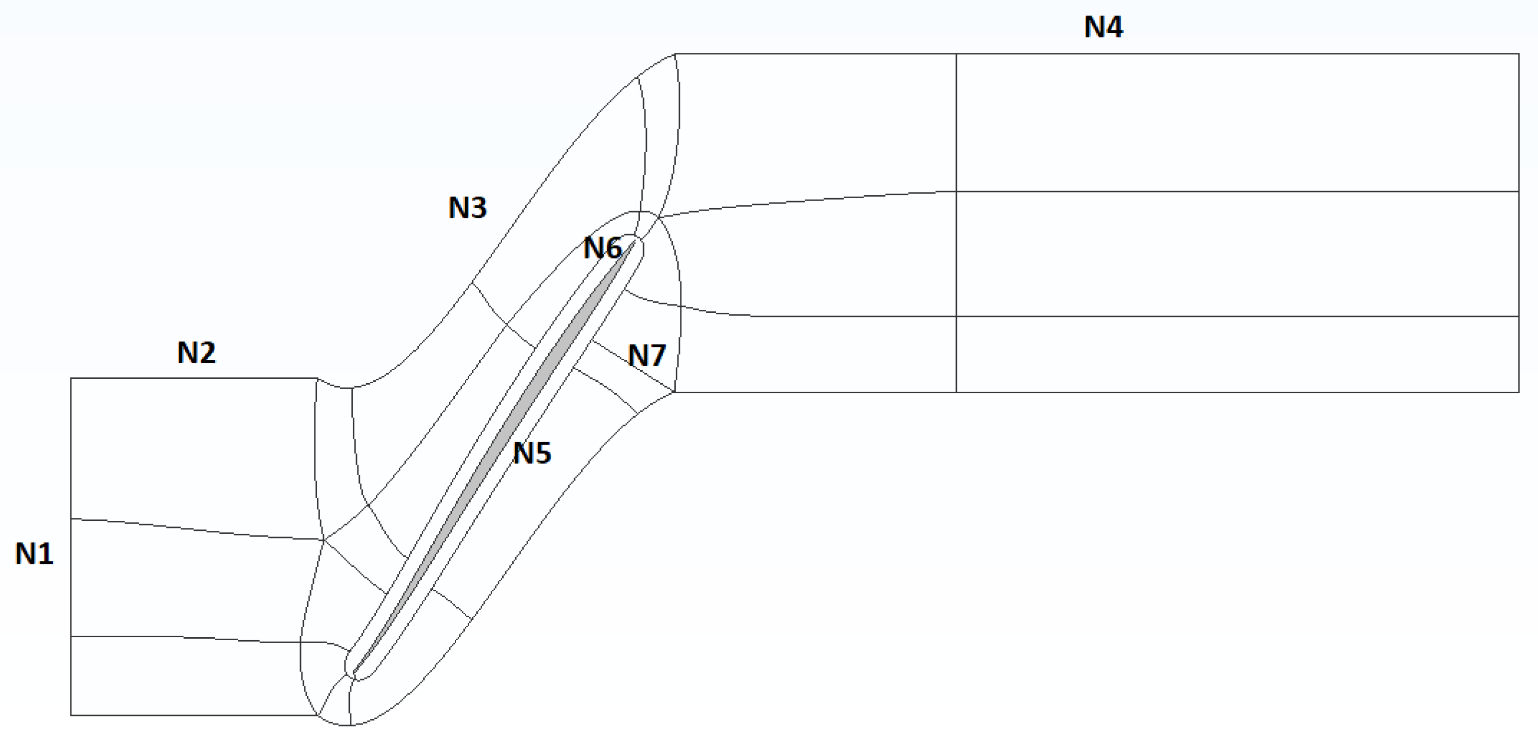
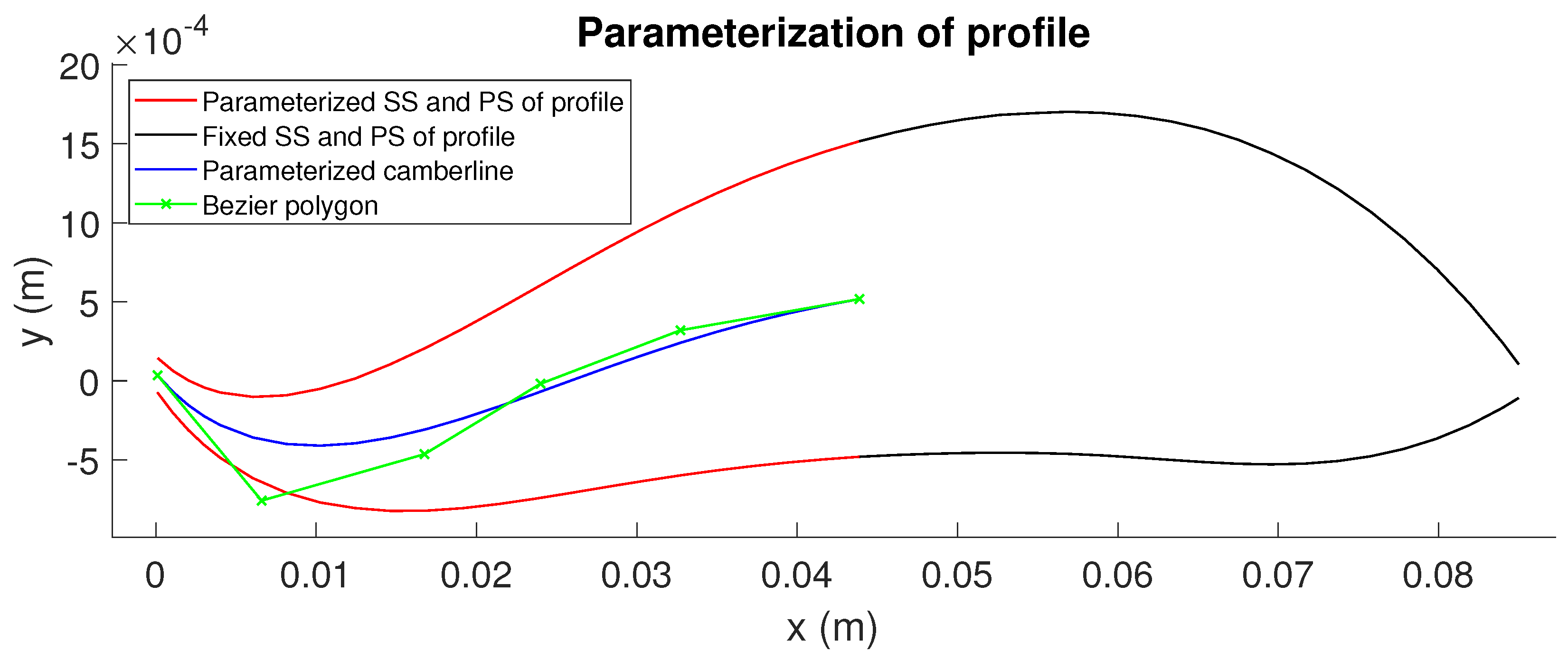
Table 2 with AVDR = 1 was chosen as the baseline case to be replicated in the validation. In such a condition, the flow was stationary, and since all the relevant quantities were measured on the simply-extruded central blade of the row, three-dimensional effects and sidewall influence were minimized. The profile, generated using a Catmull–Rom curve and semi-circular arcs for leading and trailing edges, has been inserted into a two-dimensional structured multi-block domain, extending for
upstream of the leading edge and
downstream of the trailing edge, where
is the axial projection of the chord. Around the profile, an O-grid was extruded with the number of inflation layers ranging from 100–150 depending on the grid refinement and an exponential growth rate from 1.04–1.08. The first layer height was fixed in order to get an
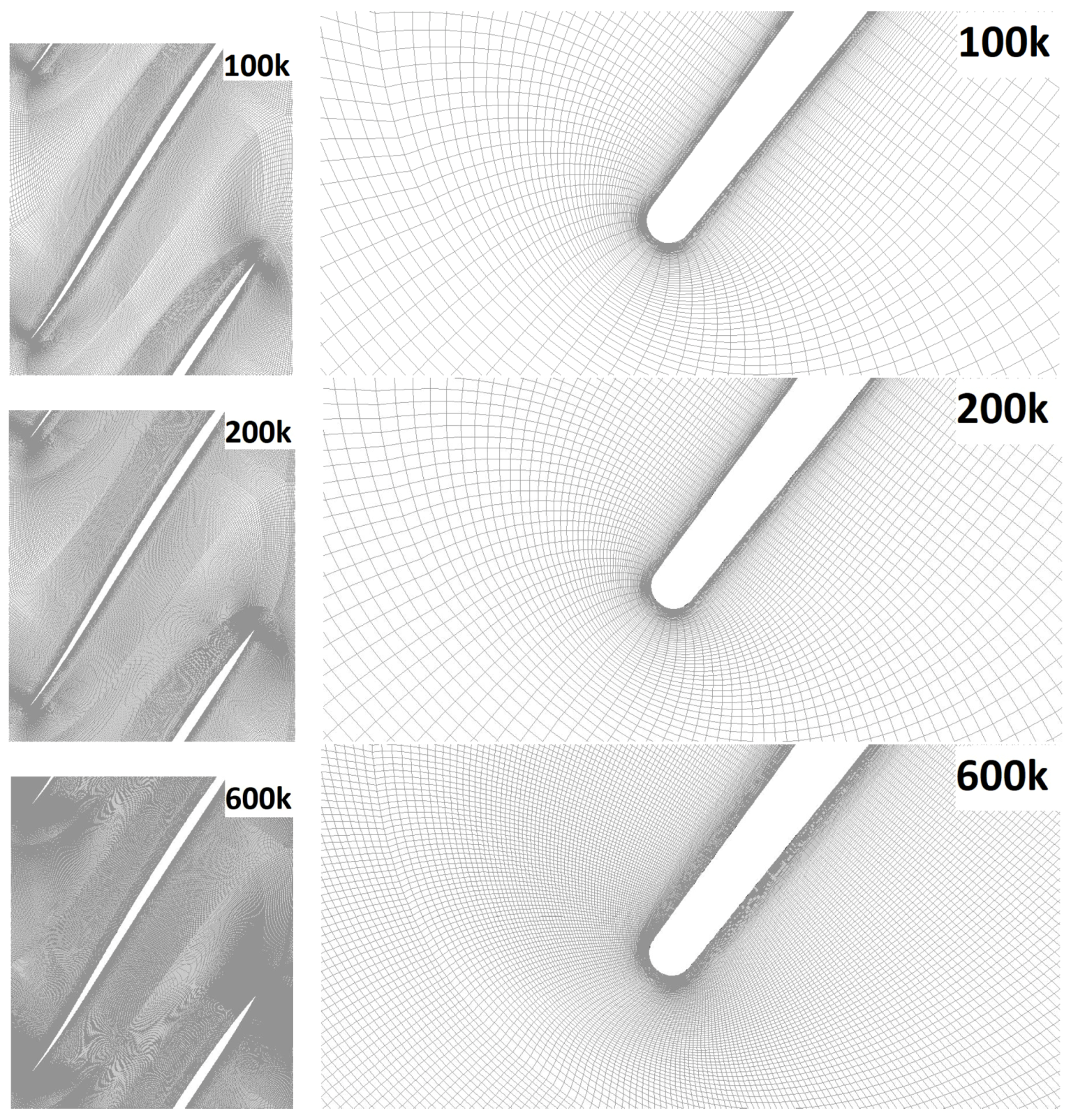
, to ensure an adequate resolution in the calculation of velocity profiles inside the boundary layer using wall functions. Three different grid sizes were tested, ranging from 100k–600k cells. In
Table 3 and
Table 4, and
Figure 1 and
Figure 2, the main features of the three grids and quality parameters are reported.
Calculations were carried out using ANSYS
TM Fluent v16 [
12], in which the Reynolds Averaged Navier-Stokes (RANS) equations coupled with a turbulence model were solved using a finite volume method approach. The solver is pressure based with a coupled scheme of resolution and Green–Gauss cell-based spatial discretization. As for the boundary conditions, a pressure far field at the inlet, with specifications of the turbulence intensity and viscosity ratio, was prescribed. Total temperature and pressure at the inlet were fixed respectively at
K and
atm; in this way, the resulting Reynolds number was
, close to the one obtained in the experiments. At the outlet, the pressure outlet was imposed; in particular,
was set during the validation phase. Blade walls were treated as walls with no slip; for the upper and lower bounds of the domain, periodic translational was prescribed in order to simulate an infinite blade row. Convergence was established when all residuals went under
, and the oscillation of the inlet Mach number, inlet flow angle, and loss coefficient were below a certain threshold. Five turbulence models were tested:
k–
Shear Stress Transport (SST) [
13],
k–
standard (STD) [
14],
k–
realizable (REAL) [
15],
k–
Re-Normalisation Group (RNG) [
16], and Spalart–Allmaras (SA) [
17] with the 100k grid. For every simulation, conditions at infinity were tuned in such a way that they could respect the experimental Mach number in the inlet section. In fact, an arbitrary choice of the inlet flow angle at infinity will generally modify the couple
at the inlet, according to the unique incidence. In
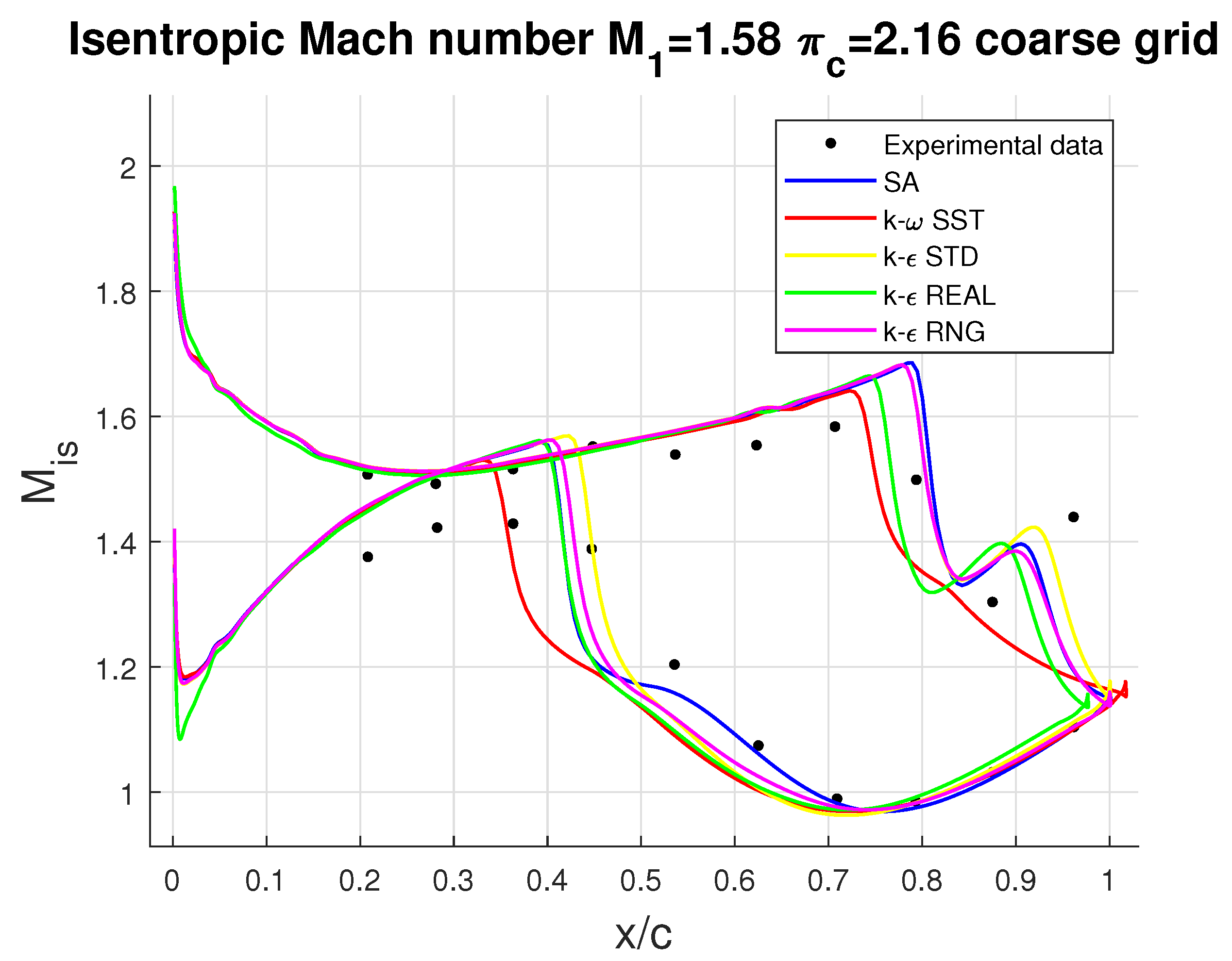
Table 5, global quantities are reported as the mass-weighted average in the section of interest for each simulated model of turbulence, while
Figure 3 shows the isentropic Mach distribution.
It can be noticed that the inlet flow angle calculated in the simulations was overestimated by about 0.5, and the same applies for the exit flow angle, probably because of the lack of accurate knowledge of the leading edge geometry. However, the mean flow deflection was well captured by the SA model and slightly less by
k–
SST and
k–
RNG. The loss coefficient was overestimated for
k–
variants, while it was underestimated for the
k–
SST. The SA model was able to get closer to the experimental
, with a slight underestimation.
k–
and the SA model replicated with better accuracy the isentropic Mach number distribution, with little anticipation of the point of incidence of the reflected shock on the suction side, while the
k–
SST model was not able to catch the re-acceleration of the flow near the trailing edge.
k–
RNG and the SA model seemed to provide better consistency with the experimental calculated loss coefficient, the isentropic Mach number distribution, and flow angles, with a slightly better agreement for the SA. In a previous work related to the same cascade [
18], the authors found that the SA model could provide an overall good match with experimental data, with similar results for
k–
. However, for the current case, the
k–
RNG model was adopted for its closer prediction of
at validation conditions and its high responsiveness to the effects of rapid strain and streamline curvature [
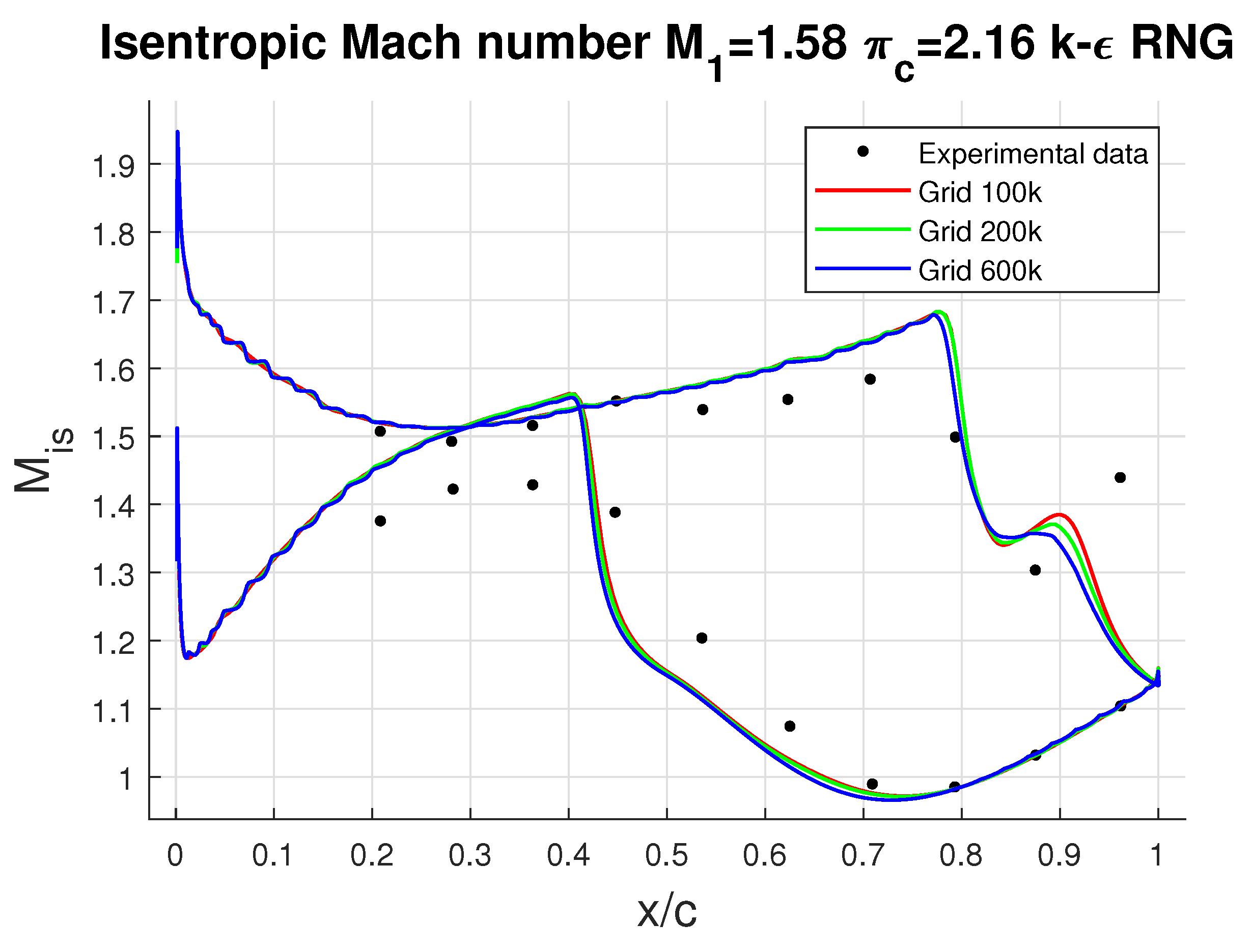
12], favorable attributes for the simulation of hooked configurations possibly arising during optimization. A sensitivity analysis towards the grid size was also carried out: two levels of grid refinement were tested, namely a 200k cell mesh and a 600k one. Results are summarized in
Table 6 and
Figure 4. It can be noted that global quantities remained substantially unchanged with respect to grid refinement, with a slightly better agreement in the loss coefficient. However, the decrease in the acceleration on the suction side near the trailing edge departed from experimental data. This small sensitivity of numerical quantities towards grid refinement suggested that the coarse grid had sufficient accuracy to ensure reliable results, with the remarkable advantage of a faster calculation over finer grids. For these reasons, it was adopted for the optimization, given the large number of simulations requested for each evaluation of the fitness functions.


