Investigation of the Trailing Edge Modification Effect on Compressor Blade Aerodynamics Using SST k-ω Turbulence Model

Abstract

A gas turbine power plant in Thailand had the problem of compressor blade fracture in Stages 6–8, which was caused by housing damage. This gas turbine has a total of 15 stages. The housing damage reduced the lifetime of blades to an unacceptable level. This article shall report the solution and outcomes. Three-dimensional (3D) compressor blade models in the problematic stages were prepared by a 3D scanning machine to find a solution based on computational fluid dynamics (CFD), and then were completed for simulation by adding Stages 5 and 9 to become a multi-stage axial model. The latter models were modified by trimming the trailing edge by 1-, 5-, and 10-mm. Using ANSYS CFX R19.2 software, the CFD results of the trailing edge modification effect on flow using the shear stress transport (SST) k-ω turbulence model revealed aerodynamics inside the problematic stages both before and after blade modifications. Modifying the blade by 5 mm was suitable, because it had lesser effects on aerodynamic parameters: pressure ratio, drag, and lift coefficients, when compared to the modification of 10 mm. The larger the modification, the greater the effect on aerodynamics. The effects on aerodynamics were intensified when they were modified by 10 mm. The validation of base line blades was conducted for the overall compressor parameters that were compared with the measurable data. These results were accepted and gave positive feedbacks from engineers who practically applied our reports in a real maintenance period of gas turbine.

1. Introduction

In the present decade, high-performance and cost reduction methods to develop modern axial compressors in a gas turbine power plant are greatly demanded. The objectives of modifications are improving the compressor blade reliability under low risks with higher loading, increasing rotational speed, and extending usage duration. The partial blade-geometry modification is one of common methods that have been applied at precise maintenance schedules. However, the modifications become a challenge in modern compressor blade because they can cause damages and disorderly aerodynamics behavior. Consequently, this unproven redesign without engineering analysis may cause high risk potentials in the failure of compressor system as well as influent to the power plant’s dependability and safety regulations. As recently reported, a gas turbine power plant of the Electricity Generating Authority of Thailand (EGAT) had been faced with a housing damage problem. This damage led to a compressor blades’ fracture. The blade’s geometry no longer suits actual operations in a current power plant, since the base line rotor-stator blade system was designed in the last decade. This outdated design had high risks of housing damage and premature crack initiation. Figure 1 shows an example of compressor blade fracture in the gas turbine that occurred at one of the EGAT’s power plants. In this power plant, the problem occurred in Stages 6–8 out of 15 stages of the gas turbine. To solve this problem, trimming trailing edge method as geometric modification had been employed. In this work, the computational fluid dynamics (CFD) was applied to investigate the sufficient trimming trailing edges and their effects on aerodynamics. This research is collaboration between the authors and EGAT to sustainably solve the problem.

Many researchers including Ning et al. [1] studied the aerodynamic analysis of the new multi-stage axial flow compressor. The results showed that large separation in the suction side of the last stator and the mainstream flow was the main factor that caused the loss. The most significant achievement of the three-dimensional (3D) blade redesign in [1] was the stall margin improvement, which totaled around 13% of stall margin when compared to the baseline, while maintaining efficiency at the design points. Bian et al. [2] investigated edge geometry with different blade parameters. The investigation precisely showed that changing the circular arc blade leads to a separation of bubbles and decreasing of the flow losses. Wei et al. [3] performed detailed experimental and numerical investigations to further comprehend the reduction mechanism of end wall secondary flow by leading-edge fillet. The results suggested that the fillet could reduce the region of corner vortex separation and eliminate the inversed flow. Gao et al. [4] continued the previous research and focused on understanding of the flow mechanisms under the tip clearance of fluid flow and the loss in variable turbine cascade. The experimental uncertainties were considered, and numerical results were conducted based on the CFD software, ANSYS CFX R11.0. The results suggested that the vane tip leakage loss increased the lateral pressure. Bakhtiari et al. [5] presented two-objective optimizations under the different operating conditions of the current baseline stator and the new 3D stator. The results showed less profile loss related to the front of the profile section; an elliptical leading edge. Additionally, it showed that thin front can significantly reduce the profile loss in the same way as a bowed design can increase resistance to corner stall, which is caused by the obtuse angle between the end wall and the suction side surface. Liu et al. [6] reported methods to improve the compressor blade design. It has been confirmed that the curvature’s discontinuities between the leading edge and the blade surface can improve the stall pressure ratio by approximately 3%. Moreover, after the blade leading edge modification, the maximum efficiency increased by approximately 1%. Razavi et al. [7] used the full compressible turbulent model to simulate the impact of sweep and to lean on the aerodynamics and performance parameters of the transonic axial flow of compressor rotors by using the systematic step-by-step procedure. The results suggested that optimized sweep angles could increase the operational safety by 30%, simultaneously increasing the efficiency and the pressure ratio by 1–2%. Neshat et al. [8] considered the two rotor geometries that were generated with different geometrical characteristics. The results concluded that stage efficiency increased by 1% for operating design, while the pressure ratio of the stage decreased by 0.01%. The blade with backward (forward) sweep has been less (higher) affected by lean. Interestingly, Wu et al. [9] confirmed that the trailing edge (TE) modification significantly improves the overall heads and pump efficiency in the high flow rate region. This finding confirmed that a small change in the TE of the impeller affects the flow structure in the impeller and it effectively improves the performance of the mixed-flow pump. Similarly, the results reported by Castegnaro [10] also presented that TE modification leads to a loss of pressure and an increase in efficiency. This work also proposed a proper shape of modification. Arbabi et al. [11] demonstrated the ability to inverse-design turbomachinery stages using the inverse method by redesigning the stators of Stages 6 and 7 to reduce the incidence angle, where the stage efficiency performed an improvement of about 0.9%. Liu et al. [12] studied the effects of compressor aerodynamic parameters, such as pitch-chord ratio, aspect ratio, and fillet on the cascade performance. The result showed that the blade with the fillet still has positive effects on the control of the corner separation, while the cascade performance with slot configuration is better than the slot configuration under the influence of the blade fillet. Dhanya and Sarath [13] performed numerical analysis to figure the effect of four tip configurations; dimpled tip, double squealer tip, pressure side squealer tip, and suction side squealer tip on plain tip. The correlation results for loss through cascade showed linear correlation between tip clearance loss and tip clearance gap as well as the dimpled tip, which reduces loss at the different tip clearances. Lu et al. [14] studied the effect of dimple’s location for a highly loaded linear compressor cascade to aerodynamics characteristic and performance. The summarized results concluded that dimples that were located on the suction surface could reduce the total pressure loss coefficient and increase the static pressure coefficient. However, the dimples beneath the separation region dramatically reduced the cascade flow condition. Choi and Ryu [15] examined the effects of axial gap to thermal and flow behavior in two-stage high pressure gas turbine. The results showed that the axial gap was the main factor that caused the damage by increasing the area-averaged heat flux to the blade surface, and the total-to-total efficiencies of the overall turbine increased while the axial gap decreased. Tao et al. [16] found that the cavitation and flow separation behavior was also related to the round and ellipse leading-edge. All of the researches mentioned above provided useful information applicable to this research, such as the shape of modification, theory, CFD calculation setup, methodology, etc.

The main objective of this work is to investigate before and after the modifications of TE effect on aerodynamics. The 3D multi-stage variable geometry was created using 3D scanning machine, with less than 5% geometry variation when compared to the actual blade. To solve the housing damage problem, the alternative models to modify the blade were proposed. The full CFD calculation of the turbulent flow with shear stress transport (SST) k-ω, including curvature correction options, were performed by ANSYS CFX R19.2 based on the finite volume method (FVM). Meanwhile, the boundary conditions were taken from actual measurable data. Numerical results after grid independent study of base line blades were compared with the EGAT’s data to confirm the results of simulation. Finally, the CFD results were investigated and then analyzed to confirm the modification’s availability.

2. Methodology

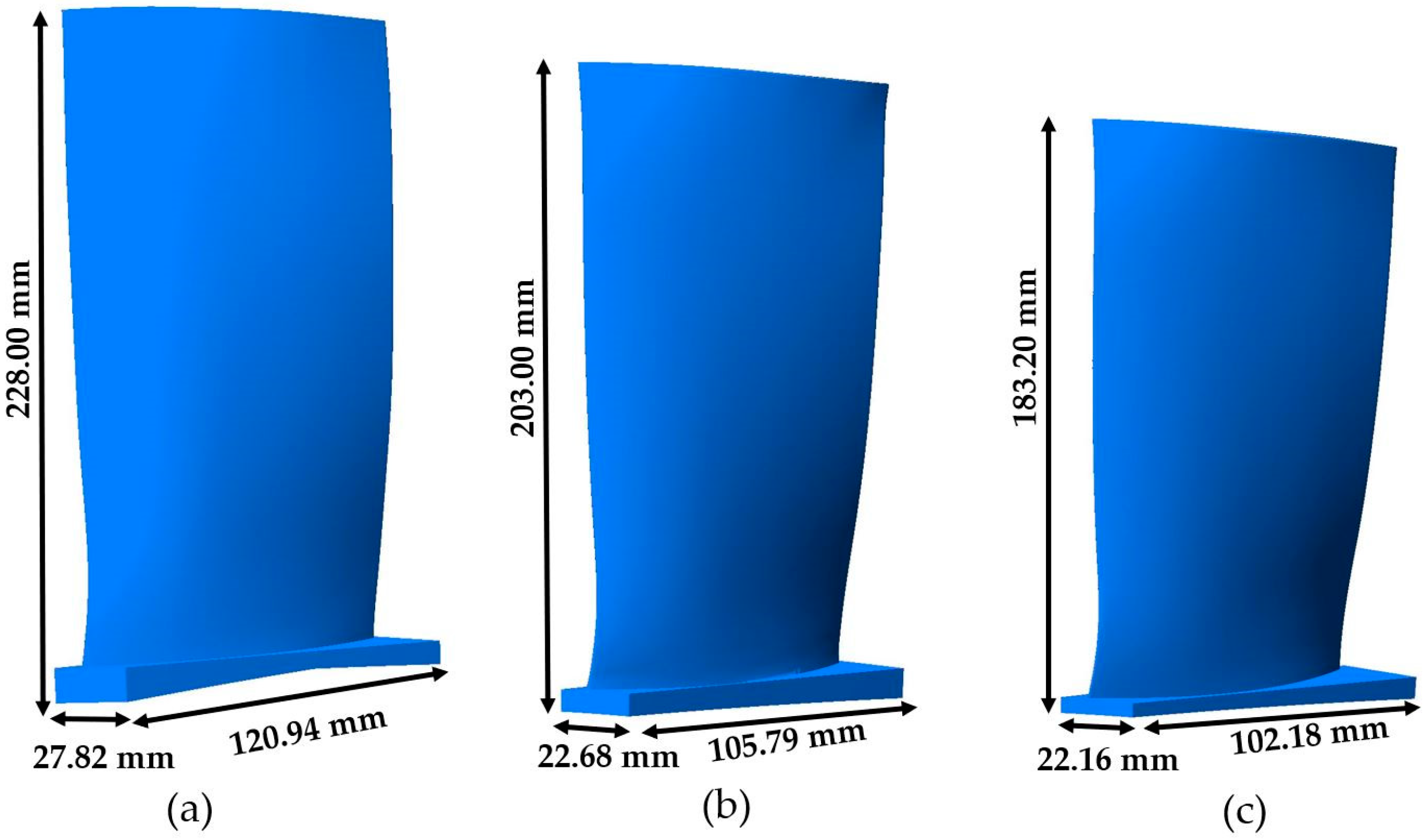
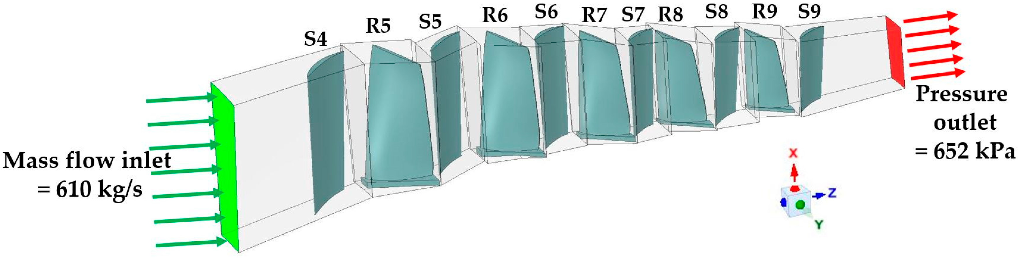
2.1. Geometry and Mesh Details

Problematic-axial compressor from one of EGAT power plants was chosen for this study. The 3D solid model was created with a FARO Edge Arm three-dimensional scanning machine in the EGAT laboratory, as shown in Figure 2a for a blade in Stage 7. Figure 2b shows a simplified model for the final simulation domain. In Figure 2a, lots of edge lines are presented on the model. To avoid the creation of poor mesh quality with many elements, a simplified model in Figure 2b was employed instead. Three simplified models for the blades in the problematic stages were created, as in Figure 3, with the different geometric dimensions of the blades at (a) Stage 6, (b) Stage 7, and (c) Stage 8, respectively. To solve the problem of the blade fracture, the shape modification of the blade, as seen in Figure 4, were proposed. Two small figures in the left show shapes of the blade before and after modifications. The modified blade was trimmed with the length of 5 mm in the diagonal direction when compared to the original-based line. In this work, trimming trailing edge of the blades at 1 mm, 5 mm, and 10 mm set the variations of the blade’s modifications. The thicknesses of the blades in the trimming regions were 6.03, 4.51 and 5.29 mm in Stages 6, 7, and 8, respectively. As the modified models were applied as prototypes, the mesh models of Stages S4–S9 were created. Thus, there are four cases in the simulation; (1) before the modification, after the modifications of (2) 1 mm, (3) 5 mm, and (4) 10 mm. Figure 4 (right figure) represented the sample of the surface mesh model with the modification of 5 mm trimming trailing edge. In an independent grid test, seven mesh models with 3.71–4.68 million nodes and 1.53–1.92 million elements were created. Each model has a difference in the number of boundary layers and the first cell size. After the independent grid test, the reasonable mesh model with 10 boundary layers and the first cell size of 1 × 10⁻³ mm for four cases were obtained. The reasonable mesh model provided results that did not change, despite increasing the number of boundary layers and decreasing the first cell size.

Table 1. Mesh details.

Domain	Nodes	Elements	No. of Blades
S4	434,398	1,880,465	63
R5	644,654	2,689,547	58
S5	413,149	1,797,943	71
R6	558,787	2,320,838	66
S6	358,677	1,520,767	73
R7	468,637	1,932,659	75
S7	307,316	1,261,484	75
R8	403,899	1,663,696	77
S8	285,277	1,214,127	79
R9	325,074	1,366,770	82
S9	237,098	1,002,103	81
All Domain	4,436,966	18,650,399	-

shows the mesh details for the simulation.

2.2. Mathematical Model

The numerical simulation was performed while using commercial CFD software, ANSYS CFX R19.2 based on Finite Volume Method (FVM) in steady state. The steady-state simulation was used when the blade was rotating at a constant speed of 3000 rpm. With this speed, there is no effect of the time to the flow field. The credibility of success from using steady-state simulation was closer to our work, such as the researches reported by Wu et al. [9] and Castenaro [10]. Subsequently, the second-order advection scheme was used for all of the turbulent transport equations and the high-resolution advection scheme was used for the set of Navier–Stokes equations [17]. Moreover, the multi-stage axial compressor was assumed to periodically rotate, only one stator and rotor impeller per passage. The mixing plane approach was carried out for the circumferential averaging of the fluxes between the stator-rotor interface. Figure 5 shows the final fluid domain for simulation and the boundary conditions. Both ends were slightly extended to avoid any errors from end correction. Without the extension of the both ends, the given results would be unreasonable. This is an effective technique that the authors must share to make the simulation successful. S and R stand for stator and rotor, respectively. The number is the number of stages that are located in the gas turbine. For example, R6 means a rotor in Stage 6, while S6 means stator in the same stage. As for other boundary conditions, the mass inlet with subsonic options that are based on isentropic relations were at the inlet of S4, while the outlet boundary conditions were used as average relative pressure at S9. Surely, the gas turbine aerodynamics simulation results are the most accurate when done in full scale with all stages, simulating in every state. As our aim is to save computational time and to reduce computer resources, and since the gas turbine had problems at Stages 6–8, primarily we simulated by using only three stages. Still, no matter which way we simulated the aerodynamics of all three stages, or how we adjusted the boundary conditions, we could not find the correct simulation results. Hence, we added S4, R5, S5, R9, and S9 into the simulation to increase the credibility.

No researches have simulated the gas turbine in certain stages to solve the problem, as mentioned in this article before. Therefore, this research acknowledges to us that, by simulating the aerodynamics of the gas turbine in certain stages, it is highly necessary to add stages before and after into the model for a more accurate answer.

2.3. Turbulence Flow of Compressible Fluid

For the accurate numerical simulation of turbulence flow characteristic, the steady state with compressible SST k-ω, including curvature correction model was performed using ANSYS CFX R19.2 based on the Reynolds-Averaged Navier–Stokes (RANS) [18]. From the previous research [18,19,20,21,22], the shear stress transport (SST) k-ω is a hybrid of the Wilcox STD k-ω in Equations (1) and (2) and transform k-ε, model in Equations (3) and (4). Menter [19,20] combined the formulations in the free stream and the k-ω formulation in the near wall region by blending function to seamlessly connect the two models. The system equations of turbulent transport for the SST k-ω model was given, as follows:

• Wilcox STD k-ω

  $$\frac{\partial \left(\rho k\right)}{\partial t}+\frac{\partial }{\partial x_j}\left(\rho U_{j}k\right)=\frac{\partial }{\partial x_j}\left[\left(\mu +\frac{{\mu }_t}{{\sigma }_{k1}}\right)\frac{\partial k}{\partial x_j}\right]+P_k-{\beta }^{\prime }\rho k\omega$$

  (1)

  $$\frac{\partial \left(\rho \omega \right)}{\partial t}+\frac{\partial }{\partial x_j}\left(\rho U_j\omega \right)=\frac{\partial }{\partial x_j}\left[\left(\mu +\frac{{\mu }_t}{{\sigma }_{\omega 1}}\right)\frac{\partial \omega }{\partial x_j}\right]+{\alpha }_1\frac{\omega }{k}{P}_k-{\beta }_1\rho {\omega }^2$$

  (2)
• Transformed k-ε,

  $$\frac{\partial \left(\rho k\right)}{\partial t}+\frac{\partial }{\partial x_j}\left(\rho U_{j}k\right)=\frac{\partial }{\partial x_j}\left[\left(\mu +\frac{{\mu }_t}{{\sigma }_{k3}}\right)\frac{\partial k}{\partial x_j}\right]+P_k-{\beta }^{\prime }\rho k\omega$$

  (3)

  $$\begin{array}{cc}\hfill \frac{\partial \left(\rho \omega \right)}{\partial t}+\frac{\partial }{\partial x_j}\left(\rho U_j\omega \right)=& \frac{\partial }{\partial x_j}\left[\left(\mu +\frac{{\mu }_t}{{\sigma }_{\omega 2}}\right)\frac{\partial \omega }{\partial x_j}\right]+2\rho \frac{1}{{\sigma }_{\omega 2}\omega }\frac{\partial k}{\partial x_j}\frac{\partial \omega }{\partial x_j}\hfill \\ & +{\alpha }_2\frac{\omega }{k}{P}_k-{\beta }_3\rho {\omega }^2\hfill \end{array}$$

  (4)

In Menter’s work [19,20], the set of steady state equations of the Willcox model was multiplied by function F₁, the transformed k-ω equations by function (1 − F₁), and the corresponding continuity equation, momentum equation, k and ω equations were added to give the BSL k-ω model, as follows:

$$\frac{\partial }{\partial x_j}\left(\rho U_j\right)=0$$

(5)

$$\frac{\partial }{\partial x_j}\left(\rho U_i{U}_j\right)=-\frac{\partial p^{\prime }}{\partial x_i}+\frac{\partial }{\partial x_j}\left[{\mu }_{eff}\left(\frac{\partial U_i}{\partial x_j}+\frac{\partial U_j}{\partial x_i}\right)\right]$$

(6)

$$\frac{\partial }{\partial x_j}\left(\rho U_{j}k\right)=\frac{\partial }{\partial x_j}\left[\left(\mu +\frac{{\mu }_t}{{\sigma }_{k3}}\right)\frac{\partial k}{\partial x_j}\right]+P_k-{\beta }^{\prime }\rho k\omega$$

(7)

$$\begin{array}{c}\frac{\partial }{\partial x_j}\left(\rho U_j\omega \right)=\frac{\partial }{\partial x_j}\left[\left(\mu +\frac{{\mu }_t}{{\sigma }_{\omega 3}}\right)\frac{\partial \omega }{\partial x_j}\right]+\left(1-F_1\right)2\rho \frac{1}{{\sigma }_{\omega 2}\omega }\frac{\partial k}{\partial x_j}\frac{\partial \omega }{\partial x_j}\\ +{\alpha }_3\frac{\omega }{k}{P}_k-{\beta }_3\rho {\omega }^2\end{array}$$

(8)

where

$$p^{\prime }=p+\frac{2}{3}\rho k+\frac{2}{3}\left(\mu +{\mu }_t\right)\frac{\partial U_k}{\partial x_k}$$

(9)

$$P_k={\mu }_t\left(\frac{\partial U_i}{\partial x_j}+\frac{\partial U_j}{\partial x_i}\right)\frac{\partial U_i}{\partial x_j}-\frac{2}{3}\frac{\partial U_k}{\partial x_k}\left(3{\mu }_t\frac{\partial U_k}{\partial x_k}+\rho k\right)$$

(10)

The k-ω based on the SST model accounted for the transport of the turbulent shear stress and gave highly accurate predictions of the onset and the amount of flow separation under adverse pressure gradients. The proper transport behaviour can be obtained by a limited formulation of the eddy-viscosity:

$${\mu }_t=\frac{0.31k\rho }{\max \left(0.31\omega ,S{F}_2\right)}$$

(11)

The coefficients ${\sigma }_{k3},{\sigma }_{\omega 3},{\alpha }_3$, and ${\beta }_3$ are obtained from blending function $F_1$, as follows:

$$F_1=\tanh \left({\arg }_1^4\right)$$

(12)

$$F_2=\tanh \left({\arg }_2^2\right)$$

(13)

$${\arg }_1=\min \left(\max \left(\frac{\sqrt{k}}{{\beta }^{\prime }\omega y},\frac{500\upsilon }{y^2\omega }\right),\frac{4\rho k}{C{D}_{k\omega }{\sigma }_{\omega 2}{y}^2}\right)$$

(14)

$${\arg }_2=\max \left(\frac{2\sqrt{k}}{{\beta }^{\prime }\omega y},\frac{500\upsilon }{y^2\omega }\right)$$

(15)

$$C{D}_{k\omega }=\max \left(2\rho \frac{1}{{\sigma }_{\omega 2}\omega }\frac{\partial k}{\partial x_j}\frac{\partial \omega }{\partial x_j},1.0\times {10}^{-10}\right)$$

(16)

$${\varphi }_3=F_1{\varphi }_1+\left(1-F_1\right){\varphi }_2$$

(17)

The transport equation of SST k-ω with curvature correction model is still similar to SST k-ω model. Yet, the production term was multiplied by f_r1 to f_r1P_k in Equation (7) and α₂(ωk⁻¹) f_r1P_k in Equation (8). The f_r1 formulation was given by:

$$f_{r1}=\max \left(\min \left(\left(1+c_{r1}\right)\frac{2r^{\ast }}{1+r^{\ast }}\left(1-c_{r3}{\tan }^{-1}\left(c_{r2}\tilde{r}\right)\right)-c_{r1},1.25\right),0.0\right)$$

(18)

$$r^{\ast }=\frac{S}{\Omega }$$

(19)

$$\tilde{r}=\frac{2{\Omega }_{ik}{S}_{jk}}{\Omega D^3}\left(\frac{D{S}_{ij}}{Dt}+\left({\delta }_{imn}{S}_{jn}+{\delta }_{jmn}{S}_{in}\right){\Omega }_m^{rot}\right)$$

(20)

$$S^2=2S_{ij}{S}_{ij}$$

(21)

$${\Omega }^2=2{\Omega }_{ij}{\Omega }_{ij}$$

(22)

$$S_{ij}=\frac{1}{2}\left(\frac{\partial U_i}{\partial x_j}+\frac{\partial U_j}{\partial x_i}\right)$$

(23)

$${\Omega }_{ij}=\frac{1}{2}\left(\frac{\partial U_i}{\partial x_j}-\frac{\partial U_j}{\partial x_i}\right)+2{\delta }_{mji}{\Omega }_m^{rot}$$

(24)

$$D^2=\max \left(S^2,0.09{\omega }^2\right)$$

(25)

The coefficients of Equations (1)–(25) were as below

$$\begin{array}{cccc}{\alpha }_1=\frac{5}{9},& {\beta }_1=\frac{3}{40},& {\sigma }_{k1}=1.176,& {\sigma }_{\omega 1}=2,\\ {\alpha }_2=0.44,& {\beta }_2=0.0828,& {\sigma }_{k2}=1,& {\sigma }_{\omega 2}=\frac{1}{0.856},\\ a=\sqrt{3},& c_{r1}=1.0,& c_{r2}=1.0,& c_{r3}=1.0\end{array}$$

(26)

More details and descriptions for Equations (1)–(26) can be found in Turbulence and Wall Function Theory [21].

2.4. Initial and Boundary Conditions

The initialization of the rotating axial compressor defined the boundary value problems. The following boundary conditions were measured from actual operation conditions at the power plant. In this work, the actual air mass flow inlet and mass flow outlet were used. On the inflow boundary, we set the flow regime to subsonic of ideal gas options with 610 kg/s mass flow rate, non-zero gradient of turbulence intensity, and a total temperature of 425 K. On the out-flow boundary, the average relative pressure 652 kPa and the domain interface between the stator-rotor used generic option with mixing-plane option, the pitch change was selected to pitch ration. The rotational speed of the blade was 3000 rpm. The referenced velocity was 432.867 m/s, as calculated from inlet-boundary condition by the program. Reference velocity is the mean velocity that is essentially used to calculate the drag and lift coefficients. The CFX software automatically calculated turbulence intensity and length scale. Furthermore, the shroud, hub, and blade were set to be the no-slip wall condition.

2.5. Numerical Investigation

This section presents a numerical simulation of turbulence fluid flow in rotational axial compressor. The mean continuity equation, the RANS equations, and the Menter’s SST k-ω model were solved in rotating Eulerian reference frame. A tetrahedral mesh with automatic curvature refinement was used for the whole simulation domain. The total number of mesh after grid independent test was 18.65 million, as reported in Table 1 with y⁺ less than 5, the accuracy of base line case was verified by the experimental data from EGAT. The computational resource is 16 cores of Intel Xeon 2.20 GHz with 64 GB of RAM, which required 24 h per case.

3. Results and Discussion

3.1. Validation Study

An investigation of the compressible flow with turbulence model in rotating reference frame required the reliable numerical validation that can fully describe the complex flow phenomena occurring in the flow system. The first task undertaken for evaluation of the numerical domain with base line blade in S5-R6-S6-R7-S7-R8-S8 using ANSYS CFX R19.2 found unreliable results in R6-S6-R7-S7-R8-S8 when compared to the measurement. According to the unrealistic boundary conditions, the variable domain has been re-configured to the finalized one, which includes S4-R5-S5-R6-S6-R7-S7-R8-S8-R9-S9, as previously shown in Figure 5 and mentioned in Section 2.2. The pressure and temperature results in each state after including S4-R5-S5-R6-S6-R7-S7-R8-S8-R9-S9 for the blade before modification are shown in Figure 6 and Figure 7, respectively. For the result of pressure, the greatest difference between the results from the experiment and the simulation was classified in Stage 7 at the value of 12.31%. For the result of temperature, the greatest difference was 4.23%, which also was classified in Stage 7. However, all of the simulation results were in the error bar, indicating that the numerical simulation is consistent with the measurement. The error bar came from a specification in user’s manual of the gas turbine provided by the commercial vender. The conclusion of our numerical setting, boundary conditions, and 3D domain configuration can capture important aerodynamics parameters in the rotating reference frame.

The CFD results were lower than the measurement. The difference may occur from the number of stages used. We began the simulation with S4 to S9, only 5.5 stages instead of all 15 stages of the gas turbine. If the simulation included Stages 1–3 and R4, or was calculated in all stages, we were confident that the difference would be decreased. However, in our experience, simulating the airflow in only 5.5 stages did not alter the outcomes of this research. From all mentioned above, we believe that the simulation provides credible and accurate results.

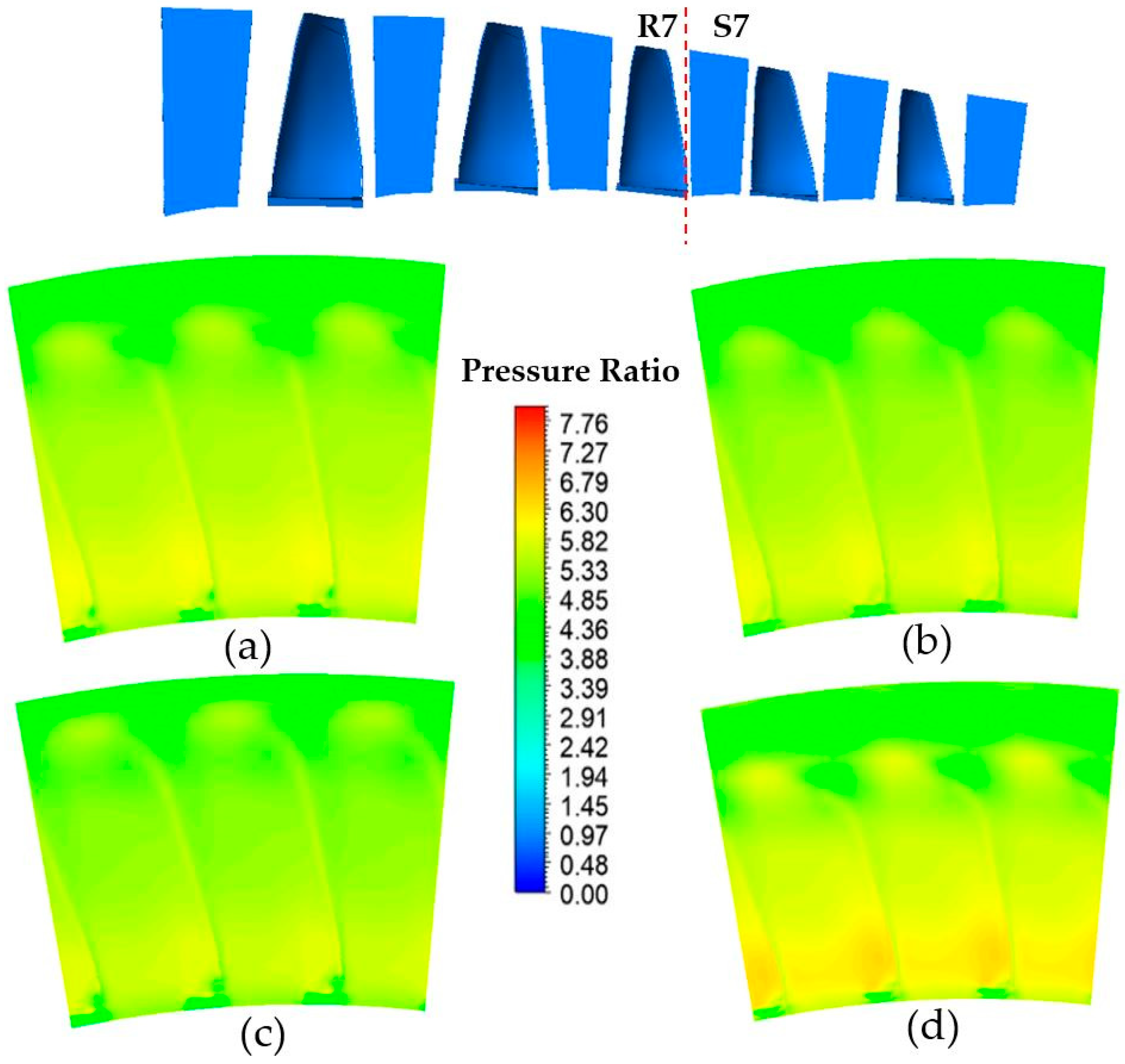
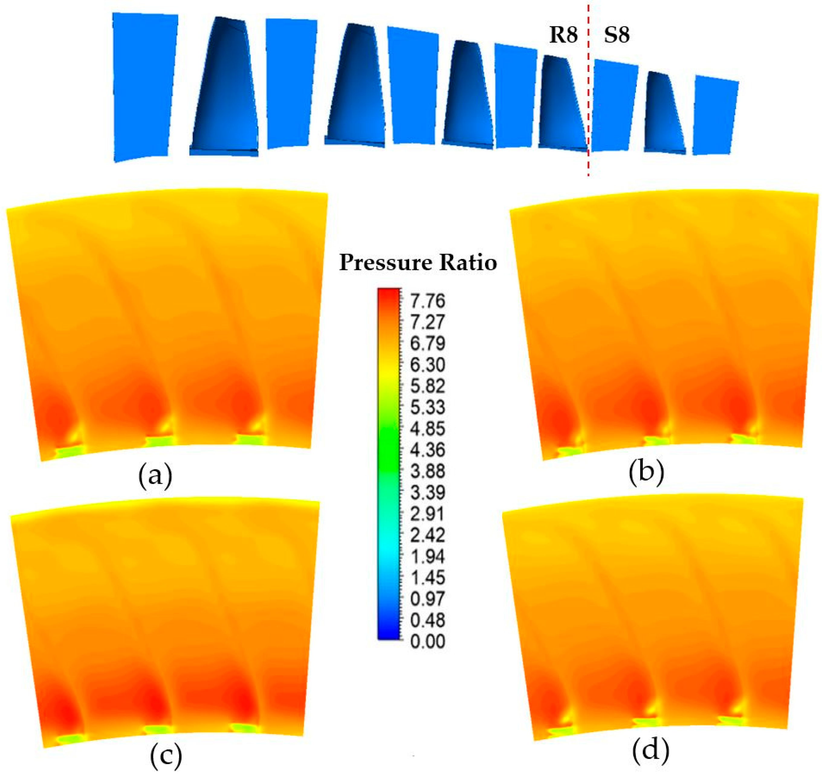
3.2. Fluid Flow in Rotational Domain

To find the CFD results, the 3D domain of axial compressor with three different trailing edge modifications, as shown in Figure 3, Figure 4 and Figure 5, were employed. In this work, an element-based finite volume method was employed, which first involved discretizing the spatial domain while using the mesh. This mesh is used to construct the finite volumes that are used to conserve relevant quantities, such as mass, momentum, and energy. Analytical solutions to the Navier–Stokes equations exist for only the simplest of flows under ideal conditions. To obtain solutions for complex flows, the numerical approach must be adopted, whereby the equations are replaced by algebraic approximations that can be solved using a numerical method.

Table 2. Numerical setting.

Numerical Parameters	Setting
Solver	Pressure-based
Special discretization	High resolution scheme for advection term
	High resolution scheme for turbulence quantities
Convergence control	Max. Iteration 1000
Convergence criteria	1.0 × 10−4
Time scale control	Auto Timescale
Length scale option	Conservative
Time scale factor	Auto Timescale

provides the assigned values of model and numerical setting.

For steady-state problems, the CFX-Solver applied a false timestep as a means of under-relaxing the equations, as they iterated towards the final solution. Due to the solver formulation being robust and fully implicit, an Auto Timescale is a fluid timescale control option that uses an internally calculated physical time scale that is based on the boundary conditions, flow conditions, physics, and domain geometry. When using the Auto Timescale option for fluid domains in a steady-state simulation, the Length Scale Option may also be used to evaluate a time scale. To avoid the excessive computational time, the maximum iteration was set to 1000 iterations. However, in our work, the solution met the convergence criteria 10⁻⁴ at 918 iterations, so the calculation was stopped. We obtained accurate results. Readers should read the Basic Solver Capability Theory for further details on setting other parameters [22].

Subsequently, the effect from trimming the trailing edge was considered based on flow field analysis. The pressure ratio (p/p_a) and velocity distribution were used to describe the flow field. The drag (C_d) and lift (C_l) coefficients represented the aerodynamic parameters in this study. Focusing on pressure ratio of the modification of R6, R7, and R8, Figure 8 shows the pressure ratio between the middle plane of R6 and S6 for the blade (a) before modification, after modifications of (b) 1 mm, (c) 5 mm, and (d) 10 mm. As shown in Figure 8, the result of R6–S6 interface obtained from turbulent flow model, high pressure ratio appeared to have a 5% increase at the hub corner in the 10 mm trailing trimming, as well as at the top of trailing edge, indicating that the maximum pressure ratio appears in lower positions than other cases. It means that the modification effect pressured field distribution in the radial direction. The same behavior is also observed in the results of R7–S7 and R8–S8, as shown in Figure 9 and Figure 10, respectively. This phenomenon tends to lead to non-symmetry pressure forces impacting the turbine, which may cause force fluctuation that affects vibration. However, we still lack the characteristics to validate the vortex dynamics, since this is a steady-state study. Comparing the pressure ratio in Figure 8, Figure 9 and Figure 10 could confirm that increasing the number of stages increases the pressure ratio, as expected. This agrees with the gas turbine’s working principle. Fresh atmospheric air flows through the compressor causing higher pressure. The greater number of stages, the higher the pressure flowing outside.

At the beginning of this research, for the purpose of convenience, we experimented with using k-ω and k-ε, turbulence models. However, the simulation results were not accurate when compared to the actual measurements—even though some stages were added, as described in Section 2.2. After we switched to using the SST k-ω, the simulation results became more accurate. The mentioned issues were consistent to Simões et al. [23], Yin et al. [24], Boretti [25], and Sonoda et al. [26], who were successful in using the SST k-ω to simulate the aerodynamics of turbomachinery applications in a steady state. Therefore, it may be concluded that the SST k-ω is a suitable turbulence model for simulating rotating turbomachinery, such as this research, as it yields credible results within the time and computer performance limitations. In Figure 8, Figure 9 and Figure 10, it was noticeable that the pressure was very high at the hub corner and at the top of trailing edge, especially when the modification included increasing the size, which also intensified the pressure. This very high pressure in the mentioned regions complied with the researches by Neshat et al. [8], Wu et al. [9], Castegnaro [10], and Halder et al. [27]. All of their studies [8,9,10,27] simulated the aerodynamics of turbomachinery, solely in a single stage. Contrastingly, our research used the SST k-ω in a multi-stage axial model to simulate up to 5.5 stages of aerodynamics to solve the problem in the gas turbine as it actually occurred. As mentioned above, the authors believe that the value of this research is another example that added worth to the SST k-ω turbulence model along to presenting the methodology of simulation with the multi-stage axial model to help engineers or staffs who work with gas turbine sustainably solve compressor blade fracture problems.

Figure 11 explains the modification effect on aerodynamic parameters indicated by lift and drag coefficients of R6, R7, and R8, for the modifications of (a) 1 mm, (b) 5 mm, and (c) 10 mm, respectively. All of the results were compared to the C_l and C_d of the blade before modification. The results precisely confirmed that the maximum values appeared in the modification of 10 mm. The drag coefficients (C_d) change for +2.30% in R6, +4.94% in R7, and −0.76% in R8. The lift coefficients (C_l) change for, +5.73% in R6, +12.97% in R7, and −1.07% in R8, respectively. For all cases, the modification had less effect on the Cd in R6, R7 and R8 regions, but it had significant effect on the C_l.

Table 3. C_l and C_d for the blade before and after modifications and the parameters using in the calculation.

Stages	Fz (N)	Fy (N)	Area (m2)	Cl	Cd
Before modification
R6	866.173	857.821	0.05542	0.1362	0.1349
R7	877.440	829.332	0.04150	0.1842	0.1741
R8	725.145	755.115	0.03564	0.1773	0.1846
After modification of 1 mm
R6	941.792	891.838	0.05537	0.1481 (+8.74%)	0.1402 (+3.93%)
R7	896.533	837.688	0.04152	0.1882 (+2.17%)	0.1759 (+1.03%)
R8	725.115	755.148	0.03566	0.1773 (0.00%)	0.1846 (0.00%)
After modification of 5 mm
R6	913.889	879.026	0.05534	0.1438 (+5.58%)	0.1383 (+2.52%)
R7	953.400	858.918	0.04149	0.2003 (+8.74%)	0.1805 (−3.68%)
R8	714.005	748.08	0.03563	0.1747 (−1.47%)	0.1830 (−0.87%)
After modification of 10 mm
R6	915.914	877.969	0.05530	0.1440 (+5.73%)	0.1380 (+2.30%)
R7	991.220	870.310	0.04141	0.2081 (+12.97%)	0.1827 (+4.94%)
R8	717.413	749.50	0.03555	0.1754 (−1.07%)	0.1832 (−0.76%)

demonstrated C_l and C_d, as plotted in Figure 11, including the related parameters employed in the calculation. Results in the bracket are the percentage changes of C_l and C_d as compared to parameters of the blade before the modification. From Figure 8, Figure 9, Figure 10 and Figure 11, it can be interpreted that modifications of trailing edges with more than 5 mm significantly affect the aerodynamic parameters and change the forces of F_z and F_y. The changes of these forces affected C_l and C_d. It is possible to claim that these modifications can cause the change in power consumption, as well as the compressor performance.

The pressure ratio from numerical simulation results indicated that the modification of trailing edge by 10 mm affects pressure field distribution in the radial direction. The aerodynamics of the blade loading ratio at 95% blade span focused on modification when compared with base line. The definition of base line is the blade before modification. In Figure 12, the blade loading clearly indicated an increase of approximately 13.58% in R6, 6.55% in R7, and 11.27% in R8, respectively. However, blade loading distribution tended to give the same results, except in the R8 regime. For the modifications of 1 mm and 5 mm, the increasing values of blade loading ratio were less than those of 10 mm. The larger the modification, the greater the effect on flow characteristics. Since the modification of 10 mm affected the flow characteristics and it may be a cause of flow-induced vibration (FIV), trimming the trailing edge more than 5 mm without the effect of flow-induced vibration will be an interesting topic for future studies.

These results were submitted to the problematic power plant and EGAT’s staff accepted them. They verified our report as one of the solutions to a housing damage problem, which can be used as essential information for actual maintenance. They also claimed that this work extended the lifetime of the blades and sustainably saved more than two-million USD from maintenance cost, including 80 million USD from commercial opportunity cost.

4. Conclusions and Outlook

This article focuses on axial compressor trimming trailing edge modification and its effects on the flow field. Three-dimensional multi stage geometry that was created by 3D scan machine with less than 5% geometry variation was compared to the original blade. The full compressible fluid dynamics of turbulent flow with shear stress transport k-ω, including curvature correction option that was performed by ANSYS CFX R19.2 based on finite volume method were considered in this study. Meanwhile, the boundary conditions that were taken from actual measurements and the numerical results after an independent grid study of base line blade were compared with EGAT’s power plant data. The result of pressure ratio distribution, blade loading at 95% blade span, lift, and drag coefficients were analyzed. The interpreted results precisely confirmed that modification by trimming the trailing edge 10 mm tended to affect around 5% of the pressure ratio, 0.76–12.97% of C_l and C_d, and 6.55–13.58% of blade loading ratio, respectively. These indications suggested that modifying less than 5 mm was suitable to avoid the change in aerodynamics behavior, but we still cannot confirm to validate the axial compressor performance as data from the power plant was confidential. We still lacked the characteristics to validate flow-induced vibrations according to pressure fluctuation on flow field since this was a steady state study. Unsteady flow simulation for a vibrating compressor rotor blade can be conducted by transient blade row flutter simulations using both time integration and harmonic balance transient methods, in combination with the Fourier Transformation pitch change model. The method allowed the capabilities of multi-stage passages for all vibration modes. The blades were forced to vibrate at one of the natural frequency modes, then, the unsteady force characteristics were calculated. The aerodynamic damping parameter was calculated, allowing for the evaluation of blade flutter in later aeroelastic analysis. McMullan et al. [28] suggested that the Large Eddy Simulation (LES) results may offer advantages over traditional RANS methods when off-design conditions are considered, as well as Duchaine et al. [29], who confirmed that, if we need to conjugate heat transfer around the turbine blade, the LES gives a comprehensive view of the main flow features that are responsible for heat transfer and the separation bubble. In the future, more studies should be carried out regarding an unsteady turbulence model, such as the LES, to validate and analyze the instant of the flow characteristic effects from blade modification.

References

1. Ning, T.; Gu, C.W.; Ni, W.D.; Li, X.T.; Liu, T.Q. Aerodynamics analysis and three-dimensional redesign of a multi-stage axial flow compressor. Energies 2016, 9, 296. [Google Scholar] [CrossRef]
2. Bian, T.; Han, Q.; Sayar, S.; Feng, J.; Böhle, M. Flow loss and structure of circular arc blades with different leading edges. Adv. Mech. Eng. 2018, 10, 1–12. [Google Scholar] [CrossRef]
3. Wei, Z.J.; Qiao, W.Y.; Liu, J.; Duan, W.H. Reduction of end wall secondary flow losses with leading-edge fillet in a highly loaded low-pressure turbine. Proc. Inst. Mech. Eng. Part A. J. Power Energy 2016, 230, 184–195. [Google Scholar] [CrossRef]
4. Gao, J.; Fu, W.; Wang, F.; Zheng, Q.; Yue, G.; Dong, P. Experimental and numerical investigations of tip clearance flow and loss in a variable geometry turbine cascade. Proc. Inst. Mech. Eng. Part A. J. Power Energy 2018, 232, 157–169. [Google Scholar] [CrossRef]
5. Bakhtiari, F.; Wartzek, F.; Leichtfuß, S.; Schiffer, H.P.; Goinis, G.; Nicke, E. Design and optimization of a new stator for the Transonic Compressor Rig at TU Darmstadt. In Proceedings of the Deutscher Luft- und Raumfahrtkongress, Rostock, Sweden, 22–24 September 2015. [Google Scholar]
6. Liu, B.; Tao, Y.; Yu, X. Application of MCST method to design the blade leading edge in axial compressors. In Proceedings of the 6th International Symposium on Fluid Machinery and Fluids Engineering (ISFMFE), Wuhan, China, 22–25 October 2014. [Google Scholar] [CrossRef]
7. Razavi, S.R.; Sammak, S.; Boroomand, M. Multidisciplinary design and optimizations of swept and leaned transonic rotor. J. Eng. Gas Turbines Power 2017, 139, GTP-17-1155. [Google Scholar] [CrossRef]
8. Neshat, M.A.; Akhlaghi, M.; Fathi, A.; Khaledi, H. Investigating the effect of blade sweep and lean in one stage of an industrial gas turbine’s transonic compressor. Propul. Power Res. 2015, 4, 221–229. [Google Scholar] [CrossRef]
9. Wu, D.; Yan, P.; Chen, X.; Wu, P.; Yang, S. Effect of trailing-edge modification of a mixed-flow pump. ASME. J. Fluids Eng. 2015, 137, 101205. [Google Scholar] [CrossRef]
10. Castegnaro, S. Effects of NACA 65-blade’s Trailing edge modifications on the performance of a low-speed tube-axial fan. Energy Procedia 2015, 82, 965–970. [Google Scholar] [CrossRef]
11. Arbabi, A.; Ghaly, W.; Medd, A. Aerodynamic inverse blade design of axial compressors in three-dimensional flow using a commercial CFD program. In Proceedings of the ASME Turbo Expo 2017: Turbomachinery Technical Conference and Exposition, Charlotte, NC, USA, 26–30 June 2017. [Google Scholar]
12. Liu, Y.; Sun, J.; Tang, Y.; Lu, L. Effect of slot at blade root on compressor cascade performance under different aerodynamic parameters. Appl. Sci. 2016, 6, 421. [Google Scholar] [CrossRef]
13. Dhanya, C.S.; Sarath, R.S. Numerical analysis of turbine tip modifications in a linear turbine cascade. In IOP Conference Series: Materials Science and Engineering; IOP Publishing Ltd.: Bristol, UK, 2018; Volume 377, p. 012051. [Google Scholar] [CrossRef]
14. Lu, H.W.; Yang, Y.; Guo, S.; Huang, Y.X.; Wang, H.; Zhong, J.J. Flow control in linear compressor cascades by inclusion of suction side dimples at varying locations. Proc. Inst. Mech. Eng. Part A. J. Power Energy 2018, 232, 706–721. [Google Scholar] [CrossRef]
15. Choi, M.G.; Ryu, J. Numerical study of the axial gap and hot streak effects on thermal and flow characteristics in two-stage high pressure gas turbine. Energies 2018, 11, 2654. [Google Scholar] [CrossRef]
16. Tao, R.; Xiao, R.; Wang, Z. Influence of blade leading-edge shape on cavitation in a centrifugal pump impeller. Energies 2018, 11, 2588. [Google Scholar] [CrossRef]
17. Barth, T.J.; Jespersen, D.C. The design and application of upwind schemes on unstructured meshes. In Proceedings of the 27th Aerospace Sciences Meeting, Reno, NV, USA, 9–12 January 1989. [Google Scholar]
18. Ali, S.; Elliott, K.J.; Savory, E.; Zhang, C.; Martinuzzi, R.J.; Lin, W.E. Investigation of the performance of turbulence models with respect to high flow curvature in centrifugal compressors. J. Fluids Eng. 2015, 138, 051101. [Google Scholar] [CrossRef]
19. Menter, F.R. Two-equation eddy-viscosity turbulence models for engineering applications. AIAA J. 2007, 32, 1598–1605. [Google Scholar] [CrossRef]
20. Menter, F.R. Zonal two-equation k-ω turbulence models for aerodynamic flows. In Proceedings of the 24th Fluid Dynamics Conference, Moffett Field, CA, USA, 6–9 July 1993. [Google Scholar]
21. ANSYS, Inc. Chapter 2. Turbulence and wall function theory. In CFX-Solver Theory Guide R19.2; Ansys Inc.: Canonsburg, PA, USA, 2019; pp. 31–44. [Google Scholar]
22. ANSYS, Inc. Chapter 1. Basic Solver Capability Theory. In CFX-Solver Theory Guide R19.2; Ansys Inc.: Canonsburg, PA, USA, 2019; pp. 65–70. [Google Scholar]
23. Simões, M.R.; Montojos, B.G.; Moura, N.R.; Su, J. Validation of turbulence models for simulation of axial flow compressor. In Proceedings of the 20th International Congress of Mechanical Engineering (COBEM), Gramado, RS, Brazil, 15–20 November 2009. [Google Scholar]
24. Yin, S.; Jin, D.; Gui, X.; Zhu, F. Application and comparison of SST model in numerical simulation of the axial compressor. J. Therm. Sci. 2010, 19, 300–309. [Google Scholar] [CrossRef]
25. Boretti, A. Experimental and computational analysis of a transonic compressor rotor. In Proceedings of the 17th Australasian Fluid Mechanics Conference, Auckland, New Zealand, 5–9 December 2010. [Google Scholar]
26. Sonoda, T.; Arima, T.; Endicott, G.; Olhofer, M.; Sendhoff, B. The effect of Reynolds number on a transonic swept fan OGV in a small turbofan engine. In Proceedings of the ASME Turbo Expo 2012, Copenhagen, Denmark, 11–15 June 2012. [Google Scholar]
27. Halder, P.; Rhee, S.H.; Samad, A. Numerical optimization of wells turbine for wave energy extraction. Int. J. Nav. Archit. Ocean Eng. 2017, 9, 11–24. [Google Scholar] [CrossRef]
28. McMullan, W.A.; Page, G.J. Towards Large Eddy Simulation of gas turbine compressors. Prog. Aerosp. Sci. 2012, 52, 30–47. [Google Scholar] [CrossRef]
29. Duchaine, F.; Maheu, N.; Moureau, V.; Balarac, G.; Moreau, S. Large-Eddy Simulation and conjugate heat transfer around a low-Mach turbine blade. J. Turbomach. 2013, 136, 051015. [Google Scholar] [CrossRef]
Figure 1. An example of compressor blade fracture.
Aerospace 06 00048 g001
Figure 2. Computational solid model of axial compressor blade: (a) three-dimensional (3D) model from FARO Edge Arm, and (b) a simplified model.
Aerospace 06 00048 g002
Figure 3. The geometric dimensions of the blades at: (a) Stage 6, (b) Stage 7, and (c) Stage 8.
Aerospace 06 00048 g003
Figure 4. Shape of a rotating axial compressor blade and surface mesh model.
Aerospace 06 00048 g004
Figure 5. Final fluid domain and the boundary conditions.
Aerospace 06 00048 g005
Figure 6. Pressure comparison between measurement and simulation.
Aerospace 06 00048 g006
Figure 7. Temperature comparison between measurement and simulation.
Aerospace 06 00048 g007
Figure 8. Pressure ratio between the middle plan of R6–S6 of the blade: (a) before modification, after modifications of (b) 1 mm, (c) 5 mm, and (d) 10 mm.
Aerospace 06 00048 g008
Figure 9. Pressure ratio between the middle plan of R7–S7 of the blade: (a) before modification, after modifications of (b) 1 mm, (c) 5 mm, and (d) 10 mm.
Aerospace 06 00048 g009
Figure 10. Pressure ratio between the middle plan of R8–S8 of the blade: (a) before modification, after modifications of (b) 1 mm, (c) 5 mm, and (d) 10 mm.
Aerospace 06 00048 g010
Figure 11. Lift (Cl) and drag (Cd) coefficients of the blade in different stage after modifications of (a) 1 mm, (b) 5 mm, and (c) 10 mm.
Aerospace 06 00048 g011
Figure 12. Blade loading ratio at 95% Blade Span (a) R6, (b) R7, and (c) R8.
Aerospace 06 00048 g012